

Archived: Interstate Technical Group on Abandoned Underground Mines
An Interactive Forum
Advanced Electromagnetic Wave Technologies for the Detection of Abandoned Mine Entries and Delineation of Barrier Pillars
by
Larry G. Stolarczyk, Sc.D., President Stolar Horizon, Inc., Raton, New Mexico
Syd S. Peng, Ph.D., C.T. Holland Professor, Chairman Department of Mining Engineering, West Virginia University, Morgantown, West Virginia
Presented to Mine Safety and Health Administration (MSHA) and Office of Surface Mining Reclamation and Enforcement (OSMRE)
Contents
- Abstract
- Introduction
- Radar Instrumentation
- Electromagnetic Fields in the Coal Seam
- Coal Seam Vision with the Radio Imaging Method (RIM)
- Void Detection with Electromagnetic Wave Methods
- Stolar Radio Imaging Method in Void Detection
- 3-D RIM to Locate and Image Mine Voids
- Downhole Survey Equipment
- Phase Synchronization
- RIM Method 1 Fence-Line Confirmation of Barrier Pillar
- RIM Case Study
- Case Study Survey Procedure
- Case Study Survey Results
- Void Detection and Confirmation Electromagnetic Wave Instrumentation Under Development
- Proposed In-Mine Test Site
- Drillstring Radar (DSR) for In-Seam Guidance and Navigation
- Current In-Seam Drilling Technology
- Basic Structure of the Drillstring Radar (DSR) Tool
- Major Subsystems
- Concluding Remarks
- References
- Acknowledgements
Figures
- Traveling EM waves are composed of electric (E) and orthogonal magnetic (H) fields
- Phase shift concept of travel distance
- Energy flow in the void detection problem
- Transmitting antenna sources
- Traveling electric field components illustrate the tilt in the vertical electric field component
- Secondary magnetic fields from a void
- Surface EM gradiometer response over a void
- Survey line across a dam
- Attenuation rate (dB/ft) versus frequency
- Electrical conductivity in Siemens per meter versus frequency
- Anisotropic gas flow permeability and dielectric (
 ) constant of coal
 - Short-duration pulse radar waveform
- Radar instrumentation
- Radar with a directional coupler
- Natural waveguide for EM wave transmission
- Coal seam EM wave attenuation rate versus frequency
- Coal seam EM wave attenuation rate versus boundary rock conductivity
- Sensitivity of radio waves to changes in coal layer thickness
- Natural coal seam anomalies
- Cross section of a paleochannel
- Comparison of RIM image reconstruction methods
- Image of a paleochannel in a 1,000-ft-wide longwall panel
- Normal attenuation rates for water-filled, air-filled, and coal waveguides
- In-mine instrumentation
- In-Mine RIM-IV transmitter
- Crosswell RIM-IV reduces drilling cost
- Crosswell detection of a coal seam void
- The RIM downhole probes are lowered into vertical borings using fiber-optic cable. Stolar's RIM Instrumentation Trailer contains two (2) cable hoists, control electronics, and probe inventory.
- Receiver probe for the Downhole RIM-IV system deployed for field-testing
- Map of a mine's target area
- Diagram of RIM survey site
- Map of the old workings originating from a highwall bench
- Map of a recommended survey plan at an old-workings site
- Location and borehole pattern of tomography grid over a suspected dike
- Two-dimensional images for a 2000-ft tomography survey grid over a dike at a 1000-ft hole-to-hole separation
- Diagram of the survey area showing downhole boring location, in-mine receiver station, and transmission ray path
- Diagram of survey area showing contour map of RIM signal attenuation rate
- Detecting coal-rock interface horizons
- Cutting drum look-ahead radar sensor
- MSHA flameproof approved RMPA Horizon Sensor (HS-3) mounted on a coal cutting drum
- Horizon Sensor response
- Quecreek Mine breach
- Salt block simulation of a coal barrier pillar
- Results from the experiments in salt
- Dielectric constant measured with the Resonant Microstrip Patch Antenna (RMPA)
- In-mine demonstration sit
- Radar mapping of voids and geologic anomalies from vertical boreholes
- Detection and imaging of abandoned coal mines along boreholes
- Vertical cross section of a coal bed illustrating conventional "sidetrack" trial-and-error drilling under a paleochannel as well as the down-the-hole drill motor
- Stolar Drillstring Radar (DSR)
- Measurements-While-Drilling (MWD) drillstring radar
- Block diagram of the drillstring radar instrumentation system
Abstract
The current high level of coal production is rapidly depleting easily minable coal reserves. Future mining will gradually concentrate in thinner, deeper, and geologically adverse coal seams. Some of the mining projects will be near old works where geophysical mapping methods will be applied separately or in conjunction with drilling techniques to delineate barrier pillars and detect voids ahead of mining machines. Several electromagnetic (EM) wave methods of detection and imaging of voids, impoundment leakage pathways, and geologic anomalies in coal beds have been investigated in recent years. Surface-based survey methods include magnetotelluric and local transmitters using low frequencies and radar at high frequencies. Both reflection and transmission instrumentation have been developed for surface, borehole, and in-mine applications.
This paper has been written for decision-makers in the coal mining industry who are concerned with the detection, confirmation, and mitigation of mining hazards in advance of mining. First, a practical insight into the science of EM wave energy travel in the coal bed has been prepared to give an understanding of EM wave interaction with voids, leakage pathways, oil/gas well casings, and geologic anomalies. Second, the interaction forms observables that are detected with specialized instrumentation. The surface-based instrumentation includes EM gradiometers and radar; in-mine and borehole instrumentation includes radar and the Radio Imaging Method (RIM). This paper also describes the development of radar for horizontal directional drills and cutting drums.
Introduction
The electromagnetic (EM) theory underlying all of the void and geologic anomaly detection methods is based upon the propagation of EM wave energy from a transmitting source of EM waves to a companion receiver (1-5). In the case of the magnetotelluric surface probing methods, the transmitting sources are naturally occurring, such as lightning, earth-ionosphere resonances, and sun spots (6). The traveling EM waves are composed of transverse electric and magnetic field components, as illustrated in Figure 1.
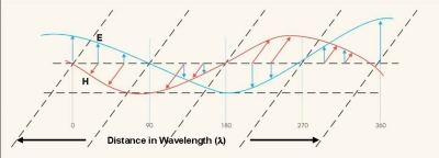
Figure 1. Traveling EM waves are composed of electric (E) and orthogonal magnetic (H) fields
The traveling field components continually exchange energy between the electric and magnetic fields along the transmission path. The distance traveled for the energy to be completely transferred to the other field component and back again is a wavelength (![]() ), mathematically represented by
), mathematically represented by
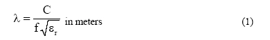
| where | C = 3 x 10⁸ is the speed of light in meters per second, |
| f = the frequency of the energy exchange in Hertz, | |
| and |
The electric and magnetic fields can be mathematically represented by sinusoidal waveforms that shift in phase by 360 electrical degrees when traveling a distance of one wavelength. The fields illustrated in Figure 1 are detected with receiving antennas. A short vertical electrical conductor is called an electric dipole and will reproduce an electromotive force (emf) voltage waveform similar to the electric field waveform mathematically expressed as
emf = hefE = M cos ![]() t (2)
t (2)
| where | hef = the effective height of the antenna, |
| E = the amplitude of the electric field in volts per meter, M = the magnitude of the sine wave signal, |
|
| and | t = the continuing time. |
A small coil of wire will reproduce an emf voltage waveform similar to the magnetic field expressed as
emf = -i![]() N
N![]() AHsin(
AHsin(![]() t)=sin M (
t)=sin M (![]() t) (3)
t) (3)
| where | N = the number of turns in the coil, i = square root of -1 A = area of coal in square meters, |
| and | H = the amplitude of magnetic field in Amperes per meter. |
If the receiving antennas were stationary, the output voltage would be continuous sine or cosine waveform. If the electric field antenna were moved a distance (d) from its original location to a new location, the reproduced waveform would be mathematically represented by
emf= M cos[![]() t +
t + ![]() ] (4)
] (4)
where ![]() = d(2
= d(2![]() /
/![]() ) is the phase shift (or rotation angle) in radians and one radian is 57 electrical degrees.
) is the phase shift (or rotation angle) in radians and one radian is 57 electrical degrees.
When the receiver moves one wavelength from its original position, the phase shift is 2![]() or 360 electrical degrees.
or 360 electrical degrees.
Distance in the natural media can be determined by designing instrumentation to measure phase shift
![]() - d(2
- d(2![]() /
/![]() ) in radians. (5)
) in radians. (5)
The braced term is called the phase constant
![]() = 2
= 2![]() /
/![]() radians per meter (6)
radians per meter (6)
and characterizes natural media.
Phase shift (or rotation angle) measurements are carried out with synchronized instrumentation. The concept of synchronization in mechanical and electronic systems is similar. For example, the cosine wave at the first location is called the reference signal. The reference signal is compared to the signal at the second location to determine the phase shift in radians.
An analogy of phase shift in EM fields traveling along a path through natural media is the rotation of a wagon wheel traveling along a path between the transmitter (source) to the receiver (Figure 2).
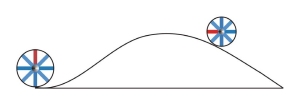
Figure 2. Phase shift concept of travel distance
As the wagon wheel rolls from the transmitter along a path (track) to the receiver, the red spoke angular rotation in degrees can be related to travel distance. In uniform natural media, the track is a straight line. The travel path of an EM wave is not always straight. EM fields are refracted when traveling near geologic anomalies where velocity changes spatial position. When the EM field receiver is synchronized with the transmitter, the total path phase shift can be measured, which is important in the problem of detecting voids and geologic anomalies ahead of mining.
The velocity of the EM field is at the speed of light in free space, but slows down in natural media. The velocity (![]() ) in a dielectric like coal is given as
) in a dielectric like coal is given as
![]()
In distance measurements, the receiver must be synchronized with the transmitter to enable the measurement of total phase shift.
Figure 3 illustrates how energy flows in natural media, such as soil, coal, and other natural media. Energy is partly transmitted and reflected when the electrical parameters of the media abruptly change. Energy is absorbed as heat in coal.
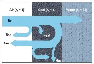
Figure 3. Energy flow in the void detection problem
Scattering of energy occurs when the void or anomaly is small compared with the wavelength. When the traveling primary EM wave (electric field EP) intersects a void or geologic anomaly, secondary EM waves (electric field ES) are formed. The secondary electric field traveling away from the air-coal interface is ESC. The secondary field traveling from the coal-water interface is ESW. Energy in the primary EM wave is converted to heat along the travel path and also transferred to the secondary EM fields. EM waves traveling nearby the anomaly are refracted. Because the secondary fields are only a small fraction of the magnitude of the primary fields, electronic instrumentation must be specifically developed to measure the secondary fields in the presence of the much larger primary field. Everywhere in the natural medium, the total fields are represented by vectors as:
Electric field ET = Ep + ES and (8)
Magnetic field HT = Hp + HS. (9)
The impedance (Z) is the ratio of the total fields given as
Z = ET/HT (10)
The transmitting antenna is the source of the primary EM fields. Low-frequency antennas are generally represented as point sources, as the physical size of these antennas is usually much smaller than their wavelength of operation and mathematically represented by dipoles (7, 8). Low frequencies are used in EM sources that operate on the earth's surface and transmit EM waves into the earth because longer wavelengths penetrate deeper in the ground. Long horizontal electric wires are electric dipoles, and loops (coils) of wire are magnetic dipoles. For frequencies in the 100s of MHz, microwave antennas are used as sources, but the depth of penetration of the signal from microwave antennas in the Earth is severely limited. The various types of transmitting sources are illustrated in Figure 4.
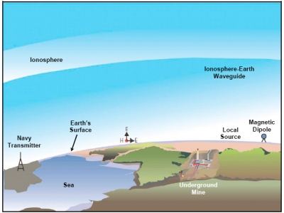
Figure 4. Transmitting antenna sources
Natural waveguides for transmission of EM waves include the earth-ionosphere waveguide illustrated in the above figure (4). The energy is transmitted with a vertically polarized electric (E) field and a horizontally polarized magnetic (H) field. The magnetic field is pointing into the page. At the air-earth interface, there is a small horizontally polarized electric field that lies on the earth's surface. The horizontally polarized E and H fields are responsible for the primary wave traveling vertically into the earth, as illustrated in Figure 5.
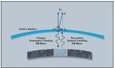
Figure 5. Traveling electric field components illustrate the tilt in the vertical electric field component
When the downward-traveling subsurface EM fields intersect a void or geologic anomaly, secondary fields form and travel back to the surface forming the total fields ET and HT at the surface. This causes the total horizontal electric field to change and the vertical electric field to tilt. The tilt would change over a void or geologic anomaly. The magnetotelluric instrumentation method measures the total horizontal electrical and magnetic field components. The surface impedance is recorded and graphically reconstructed along survey lines to form the observable in the magnetotelluric method.
EM gradiometer instrumentation has been developed for surface measurement (10). The DeltaEM gradiometer receiver is synchronized to the primary continuous wave magnetic fields traveling on the earth's surface. The DeltaEM receiver can be tuned to any frequency between 2 kHz and 2 MHz. Higher frequencies are used to detect smaller anomalies near the earth's surface. The primary wave is suppressed by more than 70 dB by differentially connected magnetic dipole antennas illustrated in Figure 6.
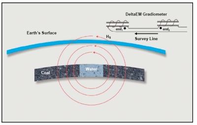
Figure 6. Secondary magnetic fields from a void
The differential (![]() ) secondary wave is measured along the survey line crossing over the void. The scattered magnetic field component traveling away from the void is mathematically given by
) secondary wave is measured along the survey line crossing over the void. The scattered magnetic field component traveling away from the void is mathematically given by
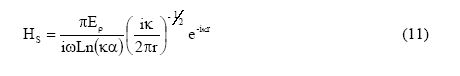
| where | |
| and | H = a cylindrically spreading magnetic field in Amperes per meter. |
Each magnetic dipole of the gradiometer array produces an output voltage given by emf0 = emf1 - emf2.
The EM gradiometer response is illustrated in Figure 7.
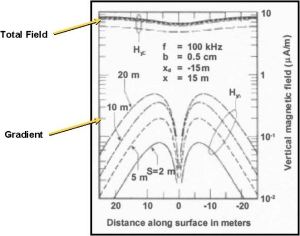
Figure 7. Surface EM gradiometer response over a void
The response illustrates the limitation in the surface-based EM measurement methods. Because the primary field is much larger than the secondary field, the total field changes by only a few percent when the survey line crosses over a significant geologic anomaly, whereas the gradient field changes by a significant amount. Surface-based instrumentation that measures total fields would exhibit poor resolution. The DeltaEM resolution is very high, which demonstrates that measuring resolution is not always related to wavelength. The wavelength in free space is 100,000 meters. The peak-to-peak separation is proportional to the depth of the anomaly (11). The DeltaEM instrumentation can be used over impoundment dams to detect leakage pathways and determine depth. A survey line across a dam is shown in Figure 8.
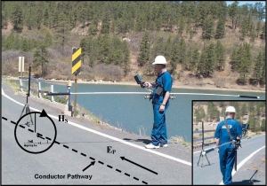
Figure 8. Survey line across a dam
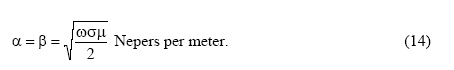
Frequently asked questions are: "What is the depth of investigation?" and "What is the resolution?" The depth of investigation strongly depends on the attenuation rate given in units of Nepers per meter (ft) for the EM fields traveling in the media and the energy lost in creating the secondary electric and magnetic field vectors. A Neper is a unit of measure defining the decrease in magnitude over the travel distance. Oliver Heaviside (12) gives a formula for determining the attenuation rate as functions of frequency, and the electrical parameters of the natural media given as
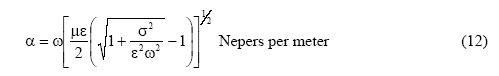
| and |
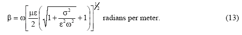
He also gave the phase shift (or rotation angle) as
When the loss tangent given by ![]() /
/![]()
![]() is much greater than unity (
is much greater than unity (![]() /
/![]()
![]() >> 1), the attenuation rate is given by
>> 1), the attenuation rate is given by
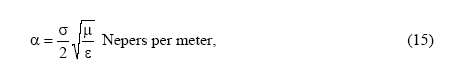
When the loss tangent is much less than unity (![]() /
/![]()
![]() << 1),
<< 1),
![]()
Figure 9 illustrates the attenuation rate as a function of frequency for a non-magnetic medium with a relative dielectric constant of 6.
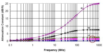
Figure 9. Attenuation rate (dB/ft) versus frequency exhibited by: a) shale/clay, b) coal with high moisture, c) range for US coals
The right side of the family of attenuation rate curves is where the loss tangent is greater than unity and the left side is where the loss tangent is much less than unity.
The significance of the loss tangent ![]() /
/![]()
![]() is seen in Maxwell's first equation, given as
is seen in Maxwell's first equation, given as
![]()
where the rotating electric field component is represented by
E = Eoe+i![]() t (18)
t (18)
and Eo is the magnitude of electric field.
The complex nature of the dielectric constant given by
![]() *=
*= ![]() ' - i
' - i![]() '' (19)
'' (19)
where ![]() ' is the real part and
' is the real part and ![]() '' is the imaginary part (13). Maxwell's first equation becomes
'' is the imaginary part (13). Maxwell's first equation becomes
![]() x H =
x H = ![]() ''
''![]() E + i
E + i![]() '
'![]() E (20)
E (20)
The first term on the right side of Equation (20) represents the conduction current (IC) flow induced in the media (IC= ![]() ''
''![]() E ohms law). We see that the electrical conductivity is given by
E ohms law). We see that the electrical conductivity is given by
![]() =
= ![]() ''
''![]() (21)
(21)
The electrical conductivity (![]() ) of sedimentary rocks has been measured in our laboratory and shows the first-order dependence on frequency as shown in Figure 10.
) of sedimentary rocks has been measured in our laboratory and shows the first-order dependence on frequency as shown in Figure 10.
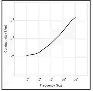
Figure 10. Electrical conductivity in Siemens per meter versus frequency
Due to the complex nature of the natural media dielectric constant, the electrical conductivity is frequency-dependent. The second term represents the electrical charge displacement current flowing in the media, the so-called capacitor effect due to the dielectric constant of the media. The loss tangent ![]() /
/![]()
![]() is the ratio of conduction to displacement current. At the microwave frequencies, displacement current will exceed the conduction current. The electrical parameters of most natural media are frequency-dependent. This fact causes the natural media to be dispersive, which means that energy travel velocity varies with frequency. In coal, the face and butt cleat structure causes the dielectric constant to be anisotropic and represented by
is the ratio of conduction to displacement current. At the microwave frequencies, displacement current will exceed the conduction current. The electrical parameters of most natural media are frequency-dependent. This fact causes the natural media to be dispersive, which means that energy travel velocity varies with frequency. In coal, the face and butt cleat structure causes the dielectric constant to be anisotropic and represented by
![]() =
= ![]() XaX +
XaX + ![]() YaY +
YaY + ![]() ZaZ (22)
ZaZ (22)
where aX, aY, aZ are unit vectors.
The dielectric constant and permeability of coal vary with the rank of coal and burial depth of the coal deposit (13). Figure 11 illustrates the anisotropic permeability and dielectric constant of coal.
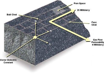
Figure 11. Anisotropic gas flow permeability and dielectric (![]() ) constant of coal
) constant of coal
Typical permeability values are 6 millidarcys orthogonal to the face cleats and 25 millidarcys orthogonal to the butt cleats.
The anisotropic dielectric constant of coal has been observed by Balanis (14) when he was a professor at West Virginia University. The anisotropic dielectric constant causes a traveling EM wave to change polarization in abruptly changing stress fields associated with high-pressure gas outburst zones. Water-filled cleats will also change polarization. Gas well casing can be detected with vertical polarization. The cross-polarization phenomena can be measured with the instrumentation and should be developed to provide additional information for mining purposes.
Radar Instrumentation
Radar (Radio-wave Detection and Ranging) instrumentation was developed during World War II to detect and track aircraft. Radar implies that transmitting and receiving antennas are collocated and operate as reflected (scattered) wave measuring instruments (15). These radar instruments solved the secondary field measuring (detection) problem by transmitted short-duration primary EM waves that traveled in free space at the constant speed of light (C) and then illuminated the target at a distance (d). The target reflects the secondary EM fields back to the radar after the round-trip travel delay time (to). The time dependence of the primary and reflected secondary radar waveform is illustrated in Figure 12.
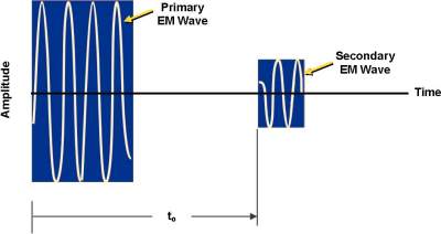
Figure 12. Short-duration pulse radar waveform
The radar instrumentation measures the round-trip travel time (to) and a rotating antenna determined the azimuth angle to the target. The travel distance to the target being tracked is given by
do = C / (2tO) (23)
The design of radar instrumentation encountered the practical problem of the high-energy primary wave leakage into the nearby receiving antenna. The high-energy leakage caused the receiving antenna and the associated electronic circuits to exhibit an impulse response. These circuits ring down as the transmitter leakage energy dissipates in the circuit. Because the sensitive radar receiver can be damaged during the ring-down time period, the receiver is switched off for a short duration of time during and following each transmission burst. This causes radar to be blinded for short distance from the radar antenna location (within the near field given by ![]() /2
/2![]() ). The far-field distance limitation occurs when the radar return (secondary EM wave) amplitude falls below the receiver inherent electrical noise. The receiver electrical noise (eN) is given by
). The far-field distance limitation occurs when the radar return (secondary EM wave) amplitude falls below the receiver inherent electrical noise. The receiver electrical noise (eN) is given by
e2N =4![]() TR BW (24)
TR BW (24)
| where | T = the temperature in Kelvin, |
R = the equivalent resistance of the receiver circuit, | |
| and | BW = the noise bandwidth in Hertz of the receiver design. |
The impulse radar transmitted EM wave exhibits a significant occupied bandwidth (BW). It is not uncommon for impulse radars to have occupied bandwidth greater than 25 MHz. The large occupied bandwidth and the dispersive nature of natural media are formidable problems for short-duration pulse radar applications in natural media. The large occupied bandwidth deteriorates maximum receiver sensitivity by the degradation factor
![]() max= 20Log10 (BW)1/2 in decibels. (25)
max= 20Log10 (BW)1/2 in decibels. (25)
The penalty paid in loss of sensitivity in a short-pulse duration radar is approximately 74 dB when compared to 1-Hz BW stepped-frequency radar receiver.
From communications theory, the optimum receiver design that maximizes the receiver sensitivity for a sinusoidal signal embedded in electrical noise is a synchronized (autocorrelation) detector (16). The synchronized receiver design drives the noise bandwidth to less than 1 Hz. It has been argued that digital sampling of the radar secondary reflected signal and digital signal processing by averaging can achieve the same receiver threshold sensitivity. This argument fails to take into consideration the digital sample's feedthrough signal limitation.
The dispersive nature of the natural media causes the occupied bandwidth frequency components to travel at different speeds, which distorts the returning secondary EM waves.
Microwave instrumentation applies transmitting antennas that are large compared to a wavelength. These systems have been developed for shallow depth of investigation. The radar instrumentation must contend with the problem that the receiving antenna is collocated with the transmitting antenna, as illustrated in Figure 13.
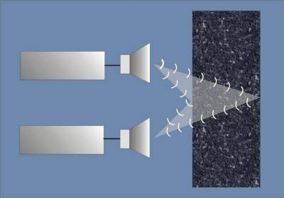
Figure 13. Radar Instrumentation
The reflected electric field component ES from the nearby air-coal interface can be determined from the reflection coefficient (![]() ) as
) as
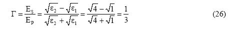
where ![]() 2 is the relative dielectric constant of the second media and
2 is the relative dielectric constant of the second media and ![]() 1 is the relative dielectric constant of the first media.
1 is the relative dielectric constant of the first media.
One third of the primary electric field (EP) is returned to the receiving antenna. The secondary electric field is only
20 Log101/3 = -9.5 dB (27)
below the primary electric field at the receiving antenna location. The secondary electric field reflected from the coal-water interface is only 7/11 of the primary electric field illuminating the coal-water interface. Coal-water interface reflected wave is itself reflected at the coal-air boundary and reduced in magnitude by one-third. The secondary electric field from the coal-water interface is
20 Log 2/3 × 7/11 × 2/3 = -10.9 dB(28)
below the primary wave. Thus, the reflected wave from the air-coal interface predominates the reflected wave from the coal-water interface. The radar instruments must be designed to measure the much smaller secondary field in the presence of the larger primary field.
Because of space limitations, directional couplers have been developed to allow a single microwave antenna to transmit and receive radar EM waves. Figure 14 is a block diagram of a radar designed with a directional coupler.
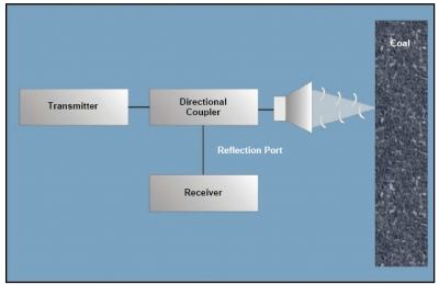
Figure 14. Radar with directional coupler.
The secondary reflected signal traveling toward the radar appears at the reflection port of the directional coupler. The receiver measures the reflected signal from the air-coal and coal-water interfaces. Directional couplers have a directivity limitation that is the leakage of the transmitter signal into the reflection port. Well-designed directional couplers exhibit a directivity of 100 dB, which is achieved with calibration algorithms.
The void secondary electric field from the coal-water interface is 16.5 dB below the primary wave. The electric fields traveling through the coal to the void and then traveling from the void to the radar antenna would be attenuated according to Figure 9. For a 100-dB directivity coupler, the available path attenuation limitation is
A = 100 -10.9 = 89.1 dB. (29)
If the average coal attenuation rate is 2 dB per ft (the highest for US coal), the detection range is at least 20 ft. In the early 1970s, Cook (17) made radar range measurements in coal mines and reported the results shown in Table 1.
| Location | Probing Distance (ft) |
|---|---|
| Pittsburgh Seam, USA | 72 |
| Virginia, USA | 66 |
| Colorado, USA | 57 |
| Ohio, USA | 33 |
| England | 23 |
The frequency domain radar overcomes the dispersive nature of natural media because the total phase shift at each frequency is measured by the radar phase-synchronized instrumentation. Since a time-domain pulse can be represented by a set of individual sine waves, the frequency domain radar sequentially generates each individual frequency component as a sinusoidal waveform signal to form the synthetic short-duration pulse waveform (18). The number of individual frequencies or steps required to reproduce the time-domain radar pulse depends on the resolution needed in the range-to-target detection. For the class of radar required in void detection, 50 steps are sufficient. The Continuous Wave Stepped Frequency (CWSF) radar frequency component is transmitted (remains on) during the ring down and the following measuring time periods, typically a few microseconds. Yet another important feature of the CWSF frequency domain radar is that synchronous (auto correlation) detection can be used to receive very small reflected signals. This capability increases the operating range and resolution compared to time-domain radar. The CWSF radar with synchronous detection can also be calibrated to make accurate reflected wave magnitude and phase shift measurements. The large dynamic range enables signal processing to locate voids in the coal bed. The phase-coherent synchronous detection of the radar electronics design enables gradational bed boundaries to be detected. Gradational bed boundaries will absorb a part of the forward-traveling radar signal, causing the reflected wave to be smaller than would otherwise be reflected from a high contrast (i.e., sharp) boundary.
The CWSF radar requires the measured frequency domain data to be transformed to the time domain. The Fast Fourier Transform (FFT) is used to determine the time-domain waveform. The transform is achieved in the digital signal processor (DSP) that receives input from the radar electronics. The FFT provides data for another algorithm for determining the distance from the drillhole to the boundary of the coal seam. This algorithm uses an adaptive decision method to determine the round trip time to each reflector (i.e., boundary). To compute the distance to the reflector boundary requires the radar to measure the dielectric constant and then correct the travel time for the dielectric constant.
Electromagnetic Fields in the Coal Seam
A natural coal seam waveguide occurs in layered sedimentary geology because the electrical conductivity of shale, mudstone, and fire clay ranges between 0.01 and 0.1 Siemens per meter (S/m) (100 and 10 ohm-meters). The conductivity of coal is near 0.0005 S/m (2,000 ohmmeters). The 10-to-1 contrast in conductivity causes a waveguide to form and waves to travel within the coal seam. The coal seam waveguide is illustrated in Figure 15.
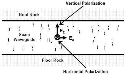
Figure 15. Natural waveguide for EM wave transmission
The electric field (EZ) component of the traveling EM wave is polarized in vertical direction and the magnetic field (Hy) component is polarized horizontally in the seam. The energy in this part of the EM wave travels laterally in the coal seam from a transmitter to a receiver. There is a horizontally polarized electric field (EX) that has zero value in the center of the seam and reaches maximum value at the sedimentary rock-coal interface. This component is responsible for transmission of the EM wave signal into the boundary rock layer. The energy in this part of the EM wave travels vertically in the coal deposit; the coal seam is a leaky waveguide. Due to this waveguide behavior, the magnitude of the coal seam radio wave decreases because of two different factors. The EM wave magnitude decreases because of the attenuation rate and cylindrical spreading of wave energy in the coal seam. The cylindrically spreading factor is mathematically given by ![]() where r is the distance from the transmitting to the receiving antenna. This factor compares with the non-waveguide far-field spherically spreading factor of 1/r. Thus, at 100 meters, the magnitude of the EM wave within the coal seam decreases by a factor of only 10 in the waveguide and by a factor of 100 in an unbounded media. An advantage of the seam waveguide is greater travel distance; another is that the traveling EM wave predominantly remains within the coal seam waveguide (coal bed).
where r is the distance from the transmitting to the receiving antenna. This factor compares with the non-waveguide far-field spherically spreading factor of 1/r. Thus, at 100 meters, the magnitude of the EM wave within the coal seam decreases by a factor of only 10 in the waveguide and by a factor of 100 in an unbounded media. An advantage of the seam waveguide is greater travel distance; another is that the traveling EM wave predominantly remains within the coal seam waveguide (coal bed).
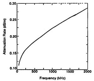 Figure 16. Coal seam EM wave attenuation rate versus frequency 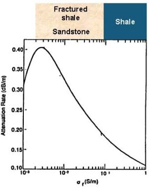 Figure 17. Coal seam EM wave attenuation rate versus boundary rock conductivity |
A coal seam EM wave is very sensitive to changes in the waveguide geology. The radio-wave attenuation rate (i.e., decibels per 100 ft) and phase shift (i.e., electrical degrees per 100 ft) were determined by Dr. David Hill (19) at the National Institute of Standards and Technology (NIST). Dr. James Wait (9) was the first to recognize that natural waveguides exist in the Earth's crust. Both researchers are Fellows of the Institute of Electrical and Electronics Engineers, Inc. (IEEE). The science underlying the traveling of an EM wave in a coal seam waveguide is well known.
The effect of attenuation in the coal seam waveguide is to reduce the magnitude of the EM wave along the path. The waveguide signal attenuation rate versus frequency is shown in Figure 16. The coal seam attenuation rate decreases with frequency. The wavelength increases as frequency decreases and the Radio Imaging Method (RIM) has greater operating range.
The effect of changing coal seam boundary sedimentary rock on attenuation rate is shown in Figure 17. Under sandstone sedimentary rock, the attenuation rate increases because more of the RIM signal travels vertically into the boundary rock, i.e., leaks from the waveguide. If water is injected into the coal from an overlying paleochannel, then clay in the coal causes the electrical conductivity and attenuation rate/phase shift to increase.
The attenuation rate/phase shift rapidly increases with decreasing seam height. The coal seam thinning can be easily detected with RIM. The graphical presentation of coal seam waveguide attenuation and phase constants in Figure 18 represents the science factor in the art and science of interpreting RIM tomographic images. Higher attenuation rate zones suggest that the coal seam boundary rock is changing, the seam is rapidly thinning, and/or water has been injected into the coal seam.
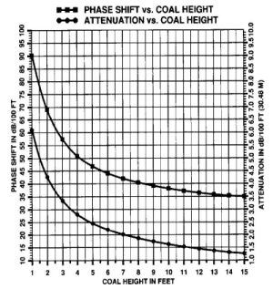
Figure 18. Sensitivity of radio waves to changes in coal layer thickness
Faults and dykes cause reflections to occur in the waveguide. The reflections can appear as excess path loss. Total phase shift measurements are useful in detecting reflection anomalies.