

- Selected Highway Capital Investment Scenarios
- Scenario Definitions
- Supplemental Scenarios
- Interstate System Scenarios
- Derivation of Scenario Investment Levels
- Investment Scenario Estimates by Improvement Type
- Investment Scenario Impacts
- Comparison of Scenario Investment Levels With Base Year Spending
- National Highway System Scenarios
- Derivation of Scenario Investment Levels
- Investment Scenario Estimates by Improvement Type
- Investment Scenario Impacts
- Comparison of Scenario Investment Levels With Base Year Spending
- Systemwide Scenarios
- Derivation of Scenario Investment Levels
- Investment Scenario Estimates by Improvement Type
- Investment Scenario Impacts
- Comparison of Scenario Investment Levels With Base Year Spending
- Supplemental Scenarios
- Scenario Definitions
- Selected Transit Capital Investment Scenarios
- Maintain Current Funding Scenario
- Rehabilitation and Replacement
- Expansion and Performance Improvement Investments
- Maintain and Improve Conditions and Performance Scenarios
- Scenario Investment Needs: Benefit-Cost Ratio of 1.0
- Investment Estimates by Asset Type
- Scenario Investment Needs: Benefit-Cost Ratio of 1.2
- Maintain and Improve Conditions and Performance Scenarios Assuming Highway Congestion Pricing
- Benefit-Cost Ratio of 1.0
- Benefit-Cost Ratio of 1.2
- Alternative Benefit-Cost Ratio Thresholds
- Maintain Current Funding Scenario
- Comparison
Selected Highway Capital Investment Scenarios
This section presents a set of future investment scenarios for highways and bridges, building on the analyses presented in Chapter 7 regarding the potential impacts of alternative levels of future investment on various measures of system conditions and performance. Each of these scenarios draw upon the results of analyses developed using the Highway Economic Requirements System (HERS) and the National Bridge Investment Analysis System (NBIAS), but also consider other types of capital investment that are currently beyond the scope of these models. This section is divided into three main parts which examine scenarios for the Interstate Highway System, the National Highway System (NHS), and the overall network of U.S. highways and bridges.
The HERS analyses presented in Chapter 7 compare the potential impacts of alternative funding mechanisms, assuming that any additional revenue needed to support a particular level of investment would be generated from one of three broad categories: non-user sources, fixed rate user based sources, or variable rate user based sources. For each scenario presented in this section, two versions are included. One version assumes that funding would be derived solely from fixed rate user based sources, while the other assumes funding from variable rate user based sources such as congestion pricing. The non-user based funding option is not explored in this section.
The technical accuracy of these scenarios depends on the validity of the technical assumptions underlying the analysis. Chapter 10 explores the impacts of altering some of these assumptions. Chapter 9 discusses some of the key implications of these scenarios. The Introduction to Part II provides critical background information needed to properly interpret these scenarios. It is important to note that each of these scenarios represents what could be achieved with a given level of investment assuming an economically driven approach to project selection, as opposed to what would be achieved given current decision making practices.
The future spending levels associated with investment scenarios presented in this chapter are all stated in constant 2006 dollars; to apply these values to a particular future year, it would be necessary to adjust them to account for actual or predicted increases in inflation beyond 2006. While the information presented in this section focuses on average annual investment levels associated with each scenario, the scenarios assume gradual increases or decreases in spending in constant dollars, as discussed in Chapter 7 [see Exhibit 7-2].
A subsequent section within this chapter explores comparable information for different types of potential future transit investments. This is followed by a section comparing key statistics from the highway and transit sections with the information presented in previous editions of this report.
Scenario Definitions
This section focuses on five selected scenarios for the Interstate System, NHS, and the overall system drawing upon the analyses presented in Chapter 7. These scenarios are intended to be illustrative; none of them is endorsed as a target level of funding. Other points along the continuum of alternative investment levels presented in Chapter 7 would be equally valid, depending on what system condition and performance outcomes are desired. Each of these scenarios are based on combined public and private investment. The question of what portion should be funded by the Federal government, State governments, local governments, or the private sector is beyond the scope of this report.
The Sustain Current Spending scenario assumes that capital spending is maintained in constant dollar terms at base year 2006 levels over the 20-year period from 2007 through 2026. The scenario also assumes that the distribution of spending will be split among the types of investments modeled in HERS, types of investments modeled in NBIAS, and types of investments that are not currently modeled, based on the 2006 base year percentages reflected in Chapter 7 [see Exhibit 7-1]. However, within the amounts reserved for HERS-modeled investment, the scenario reflects the distribution of spending that the model finds most economically attractive, and thus may differ from the actual spending distribution among resurfacing, reconstruction, and widening in 2006. Similarly, the distribution of bridge spending recommended by NBIAS may differ from the actual spending distribution among bridge repair, bridge rehabilitation, and bridge replacement in 2006.
| Why is the term "Maximum Economic Investment" applied solely to the variable rate user financing version of the MinBCR=1.0 level? | |
|
The terminology used to describe the various illustrative scenarios in the C&P Report has evolved over time to better communicate the nature of the scenarios, and to reduce the potential for confusion. For this edition, the scenarios tied to minimum benefit-cost ratios were given more technical names (i.e., "MinBCR=1.0 scenario") in order to make it easier to distinguish among them.
While previous C&P reports had used the term "Maximum Economic Investment" to describe any scenario in which a minimum benefit-cost ratio of 1.0 had been applied, the use of the term has been limited to the variable rate user financing version of the "MinBCR=1.0 scenario." This change was made to recognize that alternative financing mechanisms, as well as alternative approaches to investment decision making, can both have significant economic implications.
The variable rate financing version of this scenario reflects conditions under which users would be charged an economically rational price to travel on facilities that would be improved only to the extent that such investment was cost-beneficial.
|
|
The MinBCR=1.0 scenario assumes that combined public and private capital investment gradually increases in constant dollar terms over 20 years up to the point at which all potentially cost-beneficial investments (i.e., those with a benefit-cost ratio or "BCR" of 1.0 or higher) are funded by 2026, and the economic backlog for bridge investment is reduced to zero. This scenario represents an "investment ceiling" beyond which it would not be cost-beneficial to invest, even if available funding were unlimited. The version of this scenario assuming the widespread adoption of variable rate user charges is also described as the "Maximum Economic Investment" level, as it reflects conditions under which users would be charged an economically rational price to travel on facilities that would be improved only to the extent that such investment would be cost-beneficial.
| What are some of the technical limitations of scenarios based on minimum benefit-cost ratios? | |
|
While the MinBCR=1.0 scenarios are interesting from a theoretical technical standpoint, they do not represent practical target levels of investment for several reasons. First, available funding is not unlimited, and many decisions on highway and bridge funding levels must be weighed against potential cost-beneficial investments in other government programs and across various industries within the private sector that would produce more benefits to society. Simple cost-benefit analysis is not a commonly utilized capital investment model in the private sector. Instead, firms utilize a rate of return approach and compare various investment options and their corresponding risk. In other words, a project that is barely cost-beneficial would almost certainly not be undertaken when compared to an array of investment options that potentially produce higher returns at equivalent or lower risk. Second, these scenarios do not address practical considerations as to whether the highway and transit construction industries would be capable of absorbing such a large increase in funding within the 20-year analysis period. Such an expansion of infrastructure investment could significantly increase the rate of inflation within these industry sectors, a factor that is not considered in the constant dollar investment analyses presented in this report. Third, the legal and political complexities frequently associated with major highway capacity projects might preclude certain improvements from being made, even if they could be justified on benefit-cost criteria. In particular, the time required to move an urban capacity expansion project from "first thought" to actual completion may well exceed the 20-year analysis period.
While the MinBCR=1.2 and MinBCR=1.5 scenarios address some of these issues by screening out projects that are only marginally cost-beneficial, they still assume that projects are prioritized based on their benefit-cost ratios. That assumption is not consistent with actual patterns of project selection and funding distribution that occur in the real world. Consequently, if investment rose to these levels, there are few mechanisms to ensure these funds would be invested in projects that would be cost-beneficial. As a result, the impacts of any given budget on actual conditions and performance may be far less significant than what is projected as part of these scenarios.
|
|
The MinBCR=1.2 scenario assumes that combined public and private capital investment gradually increases in constant dollar terms over 20 years up to the point at which all potential capital improvements with a benefit-cost ratio of 1.2 or higher are funded by 2026, and the economic backlog for bridge investment is reduced to zero. This scenario was chosen to reflect that funding is not unlimited, and that targeting alternative minimum benefit-cost ratios is a reasonable method for prioritizing investments in a constrained funding environment. Applying a higher minimum benefit-cost ratio cutoff also tends to reduce the risk of investing in potential projects that might initially appear cost-beneficial, but that might not ultimately meet this standard due to unexpected changes in future costs or travel demand. It should be noted that the higher minimum-ratio cutoff applies only to those investments modeled in HERS because the benefit-cost procedures in NBIAS are not yet considered sufficiently robust to support this type of analysis. NBIAS is discussed in more detail in Appendix B.
The MinBCR=1.5 scenario assumes that combined public and private capital investment gradually increases in constant dollar terms over 20 years up to the point at which all potential capital improvements with a benefit-cost ratio of 1.5 or higher are funded by 2026, and the economic backlog for bridge investment is reduced to zero. This scenario illustrates how alternative benefit-cost ratio cutoff points in HERS can be utilized to simulate the prioritization of investments in a constrained funding environment. Other minimum benefit-cost ratio points associated with alternative funding levels are identified in Chapter 7 [see Exhibit 7-14]. The NBIAS-derived component of this scenario is based on the cost of eliminating the economic bridge investment backlog, rather than being linked to a specific minimum benefit-cost ratio cutoff point.
The Sustain Conditions and Performance scenario assumes that combined public and private capital investment gradually changes in constant dollar terms over 20 years to the point at which two key performance indicators in 2026 are maintained at their base year 2006 levels. These indicators are adjusted average user costs (as computed by HERS) and the economic backlog for bridge investment (as computed by NBIAS). They are intended to serve as summary measures of the overall conditions and performance of highways and bridges. It should be noted that while this scenario would maintain these summary indicators at base year levels for the system as a whole, the conditions and performance of individual components of the system would vary. The analyses presented in Chapter 7 identify the costs associated with maintaining several other alternative measures of system conditions and performance.
| What are some of the technical limitations of scenarios based on sustaining conditions and performance at base year levels? | |
|
The investment scenario estimates outlined in this report represent an estimate of what level of performance could be achieved with a given level of funding, not what would be achieved with it. While the models assume that projects are prioritized based on their benefit-cost ratios, that assumption is not consistent with actual patterns of project selection and funding distribution that occur in the real world. Consequently, the level of investment identified as the amount sufficient to maintain a certain performance level should be viewed as the minimum amount that would be sufficient, if all other modeling assumptions prove to be accurate.
It is important to recognize that the conditions of "today" (i.e., 2006) in this report differ from the conditions of "today" (i.e., 2004, 2002, etc.) as presented in previous editions of the report. Hence, as the level of current system conditions and performance varies over time, the investment scenarios that are based on maintaining the status quo are effectively targeting something different each time. The reader should bear this in mind when comparing the results of different reports in the series.
It should also be noted that this report uses the term "sustain" in certain scenario titles rather than the term "maintain" that has been used in previous editions. This change was made to reduce confusion, as all of these scenarios reflect capital improvements only, and do not consider routine maintenance costs.
|
|
Supplemental Scenarios
Each of the five primary scenarios described above is defined in such a manner that it can draw directly from a single HERS model run and a single NBIAS model run among the range of alternatives presented in Chapter 7. This section also includes two supplemental scenarios that draw from multiple HERS and NBIAS runs in order to estimate the costs of achieving certain objectives beyond those that can be targeted in a single analysis.
The Sustain Conditions and Performance of System Components scenario focuses on maintaining specific performance indicators for individual highway functional systems rather than more general indicators for the system as a whole. This scenario combines three elements: (1) the level of system expansion expenditures associated with maintaining average delay per vehicle mile traveled (VMT), (2) the level of system rehabilitation expenditures associated with maintaining average pavement roughness, and (3) the level of system rehabilitation expenditures associated with maintaining the economic investment backlog for bridges. This scenario does not draw directly from the analyses presented in Chapter 7. Instead, it represents a compilation of parts of many separate HERS and NBIAS analyses in which particular performances measures on particular functional systems in 2026 were maintained at base year 2006 levels.
The goal of the Sustain Conditions and Improve Performance scenario is to maintain the physical conditions of highways and bridges while improving their operational performance. This scenario represents a combination of two other scenarios; the system rehabilitation expenditures reflected in the scenario are drawn from the Sustain Conditions and Performance scenario, while the system expansion expenditures are drawn from the MinBCR=1.0 scenario.
Note that these two supplemental scenarios are presented on a systemwide basis only; comparable values for the Interstate and NHS are not separately identified.
Interstate System Scenarios
Exhibits 8-1 and 8-2 describe the derivation of the investment levels for each of five Interstate capital investment scenarios assuming fixed rate user financing and variable rate user financing, respectively. These scenarios each draw from the HERS and NBIAS analyses presented in Chapter 7. The HERS-derived scenario components link back to selected investment levels identified in Exhibit 7-18, along with the minimum benefit-cost ratio cutoff points identified in Exhibit 7-14. The NBIAS-derived scenario components tie back to selected investment levels identified in Exhibit 7-23. Each scenario covers the 20-year period from 2007 to 2026, and the investment levels shown are all stated in constant 2006 dollars.
| Scenario Name and Description | Scenario Component (And Associated Systemwide Growth Rate) * | Share of 2006 Total Capital Outlay | Average Annual Investment (Billions of 2006 Dollars) Modeled Spending |
Average Annual Investment (Billions of 2006 Dollars) Estimated Non-Modeled |
Average Annual Investment (Billions of 2006 Dollars) Total |
Share of Average Annual Investment |
|---|---|---|---|---|---|---|
| Sustain Current Spending scenario (Maintain spending at base year levels in constant dollar terms) | HERS | 77.5% | $12.8 | $12.8 | 77.5% | |
| Sustain Current Spending scenario (Maintain spending at base year levels in constant dollar terms) |
NBIAS | 15.1% | $2.5 | $2.5 | 15.1% | |
| Sustain Current Spending scenario (Maintain spending at base year levels in constant dollar terms) |
Non-Modeled | 7.4% | $1.2 | $1.2 | 7.4% | |
| Sustain Current Spending scenario (Maintain spending at base year levels in constant dollar terms) |
Total | 100.0% | $15.3 | $1.2 | $16.5 | 100.0% |
| Sustain Conditions and Performance scenario (Maintain adjusted average highway user costs and economic bridge backlog at 2006 levels) | HERS | 77.5% | $20.2 | $20.2 | 81.4% | |
| Sustain Conditions and Performance scenario (Maintain adjusted average highway user costs and economic bridge backlog at 2006 levels) |
NBIAS | 15.1% | $2.8 | $2.8 | 11.1% | |
| Sustain Conditions and Performance scenario (Maintain adjusted average highway user costs and economic bridge backlog at 2006 levels) |
Non-Modeled | 7.4% | $1.8 | $1.8 | 7.4% | |
| Sustain Conditions and Performance scenario (Maintain adjusted average highway user costs and economic bridge backlog at 2006 levels) |
Total | 100.0% | $22.9 | $1.8 | $24.8 | 100.0% |
| MinBCR=1.5 scenario (Invest in projects with BCR's as low as 1.5 and eliminate economic backlog for bridge rehabilitation) | HERS (5.03%) | 77.5% | $31.4 | $31.4 | 80.6% | |
| MinBCR=1.5 scenario (Invest in projects with BCR's as low as 1.5 and eliminate economic backlog for bridge rehabilitation) |
NBIAS (5.15%) | 15.1% | $4.7 | $4.7 | 12.0% | |
| MinBCR=1.5 scenario (Invest in projects with BCR's as low as 1.5 and eliminate economic backlog for bridge rehabilitation) |
Non-Modeled | 7.4% | $2.9 | $2.9 | 7.4% | |
| MinBCR=1.5 scenario (Invest in projects with BCR's as low as 1.5 and eliminate economic acklog for bridge rehabilitation) |
Total | 100.0% | $36.1 | $2.9 | $39.0 | 100.0% |
| MinBCR=1.2 scenario (Invest in projects with BCR's as low as 1.2 and eliminate economic backlog for bridge rehabilitation)) |
HERS (6.41%) | 77.5% | $35.6 | $35.6 | 81.8% | |
| MinBCR=1.2 scenario (Invest in projects with BCR's as low as 1.2 and eliminate economic backlog for bridge rehabilitation) |
NBIAS (5.15%) | 15.1% | $4.7 | $4.7 | 10.7% | |
| MinBCR=1.2 scenario (Invest in projects with BCR's as low as 1.2 and eliminate economic backlog for bridge rehabilitation) |
Non-Modeled | 7.4% | $3.2 | $3.2 | 7.4% | |
| MinBCR=1.2 scenario (Invest in projects with BCR's as low as 1.2 and eliminate economic backlog for bridge rehabilitation) |
Total | 100.0% | $40.3 | $3.2 | $43.5 | 100.0% |
| MinBCR=1.0 scenario (Invest in projects with BCR's as low as 1.0 and eliminate economic backlog for bridge rehabilitation) |
HERS (7.45%) | 77.5% | $38.8 | $38.8 | 82.6% | |
| MinBCR=1.0 scenario (Invest in projects with BCR's as low as 1.0 and eliminate economic backlog for bridge rehabilitation) |
NBIAS (5.15%) | 15.1% | $4.7 | $4.7 | 9.9% | |
| MinBCR=1.0 scenario (Invest in projects with BCR's as low as 1.0 and eliminate economic backlog for bridge rehabilitation) |
Non-Modeled | 7.4% | $3.5 | $3.5 | 7.4% | |
| MinBCR=1.0 scenario (Invest in projects with BCR's as low as 1.0 and eliminate economic backlog for bridge rehabilitation) |
Total | 100.0% | $43.5 | $3.5 | $47.0 | 100.0% |
| Scenario Name and Description | Scenario Component (And Associated Systemwide Growth Rate) * | Share of 2006 Total Capital Outlay | Average Annual Investment (Billions of 2006 Dollars) Modeled Spending |
Average Annual Investment (Billions of 2006 Dollars) Estimated Non-Modeled |
Average Annual Investment (Billions of 2006 Dollars) Total |
Share of Average Annual Investment |
|---|---|---|---|---|---|---|
| Sustain Current Spending scenario (Maintain spending at base year levels in constant dollar terms) |
HERS | 77.5% | $12.8 | $12.8 | 77.5% | |
| Sustain Current Spending scenario (Maintain spending at base year levels in constant dollar terms) |
NBIAS | 15.1% | $2.5 | $2.5 | 15.1% | |
| Sustain Current Spending scenario (Maintain spending at base year levels in constant dollar terms) |
Non-Modeled | 7.4% | $1.2 | $1.2 | 7.4% | |
| Sustain Current Spending scenario (Maintain spending at base year levels in constant dollar terms) |
Total | 100.0% | $15.3 | $1.2 | $16.5 | 100.0% |
| Sustain Conditions and Performance scenario (Maintain adjusted average highway user costs and economic bridge backlog at 2006 levels) |
HERS | 77.5% | $8.0 | $8.0 | 68.8% | |
| Sustain Conditions and Performance scenario (Maintain adjusted average highway user costs and economic bridge backlog at 2006 levels) |
NBIAS | 15.1% | $2.8 | $2.8 | 23.7% | |
| Sustain Conditions and Performance scenario (Maintain adjusted average highway user costs and economic bridge backlog at 2006 levels) |
Non-Modeled | 7.4% | $0.9 | $0.9 | 7.4% | |
| Sustain Conditions and Performance scenario (Maintain adjusted average highway user costs and economic bridge backlog at 2006 levels) |
Total | 100.0% | $10.8 | $0.9 | $11.6 | 100.0% |
| MinBCR=1.5 scenario (Invest in projects with BCRs as low as 1.5 and eliminate economic backlog for bridge rehabilitation) |
HERS (1.67%) | 77.5% | $17.6 | $17.6 | 73.1% | |
| MinBCR=1.5 scenario (Invest in projects with BCRs as low as 1.5 and eliminate economic backlog for bridge rehabilitation) |
NBIAS (5.15%) | 15.1% | $4.7 | $4.7 | 19.4% | |
| MinBCR=1.5 scenario (Invest in projects with BCRs as low as 1.5 and eliminate economic backlog for bridge rehabilitation) |
Non-Modeled | 7.4% | $1.8 | $1.8 | 7.4% | |
| MinBCR=1.5 scenario (Invest in projects with BCRs as low as 1.5 and eliminate economic backlog for bridge rehabilitation) |
Total | 100.0% | $22.2 | $1.8 | $24.0 | 100.0% |
| MinBCR=1.2 scenario (Invest in projects with BCRs as low as 1.2 and eliminate economic backlog for bridge rehabilitation) |
HERS (3.30%) | 77.5% | $20.8 | $20.8 | 75.6% | |
| MinBCR=1.2 scenario (Invest in projects with BCRs as low as 1.2 and eliminate economic backlog for bridge rehabilitation) |
NBIAS (5.15%) | 15.1% | $4.7 | $4.7 | 17.0% | |
| MinBCR=1.2 scenario (Invest in projects with BCRs as low as 1.2 and eliminate economic backlog for bridge rehabilitation) |
Non-Modeled | 7.4% | $2.0 | $2.0 | 7.4% | |
| MinBCR=1.2 scenario (Invest in projects with BCRs as low as 1.2 and eliminate economic backlog for bridge rehabilitation) |
Total | 100.0% | $25.5 | $2.0 | $27.5 | 100.0% |
| Maximum Economic Investment (MinBCR=1.0) scenario (Invest in projects with BCRs as low as 1.0 and eliminate economic bridge backlog) |
HERS (4.45%) | 77.5% | $23.5 | $23.5 | 77.2% | |
| Maximum Economic Investment (MinBCR=1.0) scenario (Invest in projects with BCRs as low as 1.0 and eliminate economic bridge backlog) |
NBIAS (5.15%) | 15.1% | $4.7 | $4.7 | 15.4% | |
| Maximum Economic Investment (MinBCR=1.0) scenario (Invest in projects with BCRs as low as 1.0 and eliminate economic bridge backlog) |
Non-Modeled | 7.4% | $2.3 | $2.3 | 7.4% | |
| Maximum Economic Investment (MinBCR=1.0) scenario (Invest in projects with BCRs as low as 1.0 and eliminate economic bridge backlog) |
Total | 100.0% | $28.1 | $2.3 | $30.4 | 100.0% |
For the scenarios that target minimum benefit-cost ratio cutoff points, the HERS and NBIAS components can each be linked directly to one of the 24 alternative annual percent systemwide funding growth rates analyzed in Chapter 7; the growth rates associated with these scenarios are identified in Exhibits 8-1 and 8-2. This is not the case for scenarios targeting specific spending levels or specific levels of performance (i.e., the first two scenarios in each table); as discussed in Chapter 7, the mix of investments between the Interstate system and other parts of the highway system will be different when such targets are imposed at a systemwide level than if comparable criteria were imposed on the Interstate system alone. As referenced below, certain exhibits in Chapter 7 contain "extra" rows (in addition to the standard set of alternative growth rates) to highlight the Interstate-specific funding levels.
The discussion that follows documents the derivation of the five Interstate scenarios in some detail. This information is provided to serve as a roadmap for how one could construct additional scenarios building off of different inputs from Chapter 7 beyond the selected scenarios presented here. It is important to note that these scenarios are intended to be illustrative, and any number of alternative scenarios based on different benefit-cost ratio cutoff points, performance targets, or funding targets could be constructed that would be equally valid from a technical perspective.
Derivation of Scenario Investment Levels
The average annual investment levels shown for the Interstate Sustain Current Spending scenario are identical in both Exhibits 8-1 and 8-2, and are consistent with the 2006 Interstate spending figures identified in Exhibit 7-1. This scenario assumes the continuation of the percentage splits in spending among HERS-modeled, NBIAS-modeled, and non-modeled improvement types. Of the $16.5 billion of capital investment on the Interstate System in 2006, approximately $12.8 billion (or 77.5 percent) was used for types of improvements modeled in HERS, including pavement resurfacing, pavement reconstruction, and capacity additions to the existing highway and bridge network. (The HERS-modeled impacts on adjusted user costs of sustaining the 2006 level of Interstate investment in constant dollar terms are identified for each of the funding mechanisms [non-user sources, fixed rate user charges, and variable rate user charges] in the second extra row appended to the bottom of Exhibit 7-18.) Approximately $2.5 billion (or 15.1 percent) was used for types of bridge repair, rehabilitation, and replacement improvements modeled in NBIAS. (The impacts of sustaining this level of investment in constant dollar terms are identified in the second extra row appended to the bottom of Exhibit 7-23.) The remaining $1.2 billion (or 7.4 percent) went for types of capital improvements not currently addressed by either HERS or NBIAS, including various safety enhancements, environmental enhancements, and traffic operations improvements.
Each of the Interstate System scenarios assume that the share of average annual investment directed towards non-modeled capital improvements will remain at the 2006 level of 7.4 percent. Consequently, the amounts identified as estimated non-modeled spending in Exhibits 8-1 and 8-2 are proportionally larger or smaller than the 2006 spending level of $1.2 billion, based on the change in modeled spending relative to the 2006 baseline.
| Why does the analysis assume that the share of the future highway investment scenario estimates for non-modeled items would match their share of current spending? | |
|
No data are currently available that would justify an assumption that the percentage of capital spending devoted to these investments would (or should) change in the future. In the absence of such data, it is thus reasonable to assume that their share of future investment under each scenario would approximate their share of current spending.
|
|
The average annual investment levels for the Interstate Sustain Conditions and Performance scenario for 2007 to 2026 assuming fixed rate user financing is $24.8 billion, as shown in Exhibit 8-1; Exhibit 8-2 identifies the comparable annual figure assuming the widespread adoption of variable rate user charges (i.e., congestion pricing) as $11.6 billion in constant 2006 dollars. The HERS-modeled components of these totals are $20.2 billion and $8.0 billion, respectively. (The impacts of sustaining these levels of investment in constant dollar terms over 20 years are identified in the first extra row appended to the bottom of Exhibit 7-18.) The NBIAS-modeled component is identical in both exhibits, totaling $2.8 billion because NBIAS does not consider alternative financing mechanisms. (The impacts of sustaining this level of investment in constant dollar terms are identified in the first extra row appended to the bottom of Exhibit 7-23.) The estimated non-modeled portion of the scenario differs proportionally in response to the differences between the HERS-derived figures.
As shown in Exhibit 8-1, the average annual investment level for the period 2007 to 2026 for the Interstate MinBCR=1.5 scenario assuming financing from fixed rate user charges is $39.0 billion. This includes a HERS-derived component of $31.4 billion, stated in constant 2006 dollars. (Exhibit 7-14 links the benefit-cost ratio cutoff point with an annual spending growth rate of 5.03 percent assuming fixed rate user financing, which in turn is linked to $31.4 billion of spending on HERS-modeled improvements on the Interstate system in Exhibit 7-18.) Exhibit 8-2 identifies an average annual investment for the Interstate MinBCR=1.5 scenario of $24.0 billion stated in constant 2006 dollars assuming financing from variable rate user charges, including a HERS-derived component of $17.6 billion. (Exhibit 7-14 links the benefit-cost ratio cutoff point with an annual spending growth rate of 1.67 percent assuming variable rate user financing, which in turn is linked to $17.6 billion of spending on HERS-modeled improvements on the Interstate system in Exhibit 7-18.) The $4.7 billion NBIAS-derived component shown in both Exhibits 8-1 and 8-2 represents the average annual level of investment to eliminate the economic bridge investment backlog. (Exhibit 7-23 identifies this figure, which is associated with an annual constant dollar growth rate of 5.15 percent.)
The average annual investment level over 20 years for the Interstate MinBCR=1.2 scenario assuming financing from fixed rate user charges is $43.5 billion stated in constant 2006 dollars, including a HERS-derived component of $35.6 billion, as shown in Exhibit 8-1. (This HERS component is linked to an annual spending growth rate of 6.41 percent in Exhibit 7-18, which is the rate associated with a minimum benefit-cost ratio of 1.2 in Exhibit 7-14.) Exhibit 8-2 identifies an average annual investment for the Interstate MinBCR=1.2 scenario of $27.5 billion stated in constant 2006 dollars assuming financing from variable rate user charges, including a HERS-derived component of $20.8 billion. (This HERS component is linked to an annual spending growth rate of 3.30 percent in Exhibit 7-18, which is the rate associated with a minimum benefit-cost ratio of 1.2 in Exhibit 7-14, assuming variable rate user financing.) The $4.7 billion NBIAS-derived component shown in both Exhibits 8-1 and 8-2 represents the average annual level of investment to eliminate the economic bridge investment backlog.
The average annual investment level over 20 years for the Interstate MinBCR=1.0 scenario assuming financing from fixed rate user charges is $47.0 billion stated in constant 2006 dollars, including a HERS-derived component of $38.8 billion, as shown in Exhibit 8-1. (This HERS component is linked to an annual spending growth rate of 7.45 percent in Exhibit 7-18, which is the rate associated with a minimum benefit-cost ratio of 1.0 in Exhibit 7-14.) Exhibit 8-2 identifies an average annual investment for the Interstate Maximum Economic Investment (MinBCR=1.0) scenario of $30.4 billion stated in constant 2006 dollars assuming the widespread adoption of variable user charges such as congestion pricing, including a HERS-derived component of $23.5 billion. (This HERS component is linked to an annual spending growth rate of 4.45 percent in Exhibit 7-18, which is the rate associated with a minimum benefit-cost ratio of 1.0 in Exhibit 7-14, assuming variable rate user financing.) The $4.7 billion NBIAS-derived component shown in both Exhibits 8-1 and 8-2 represents the average annual level of investment to eliminate the economic bridge investment backlog.
Investment Scenario Estimates by Improvement Type
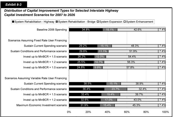
Exhibit 8-3 compares the distribution of highway and bridge capital outlay among the 20-year Interstate capital investment scenarios defined in Exhibits 8-1 and 8-2. The amounts identified as the bridge portion of the System Rehabilitation category correspond to the NBIAS-modeled portion of each scenario, while System Enhancement spending corresponds to the non-modeled portion of each scenario as estimated in Exhibits 8-1 and 8-2. The HERS-modeled portion of each scenario is split between the System Expansion category and the highway portion of the System Rehabilitation category.
| Scenario Name and Description | Average Annual Investment (Billions of 2006 Dollars) | |||||
|---|---|---|---|---|---|---|
| System Rehabilitation Highway 1 |
System Rehabilitation Bridge 2 |
System Rehabilitation Total |
System Expansion 3 | System Enhancement | Total | |
| Baseline 2006 Spending | $5.8 | $2.5 | $8.3 | $7.1 | $1.2 | $16.5 |
| Scenarios Assuming Fixed Rate User Financing | ||||||
| Sustain Current Spending scenario | $4.8 | $2.5 | $7.3 | $8.0 | $1.2 | $16.5 |
| Sustain Conditions and Performance scenario | $7.3 | $2.8 | $10.1 | $12.9 | $1.8 | $24.8 |
| Invest up to MinBCR = 1.5 scenario | $10.2 | $4.7 | $14.9 | $21.2 | $2.9 | $39.0 |
| Invest up to MinBCR = 1.2 scenario | $11.1 | $4.7 | $15.8 | $24.5 | $3.2 | $43.5 |
| Invest up to MinBCR = 1.0 scenario | $11.7 | $4.7 | $16.3 | $27.2 | $3.5 | $47.0 |
| Scenarios Assuming Variable Rate User Financing | ||||||
| Sustain Current Spending scenario | $6.4 | $2.5 | $8.9 | $6.4 | $1.2 | $16.5 |
| Sustain Conditions and Performance scenario | $4.2 | $2.8 | $7.0 | $3.8 | $0.9 | $11.6 |
| Invest up to MinBCR = 1.5 scenario | $8.0 | $4.7 | $12.7 | $9.5 | $1.8 | $24.0 |
| Invest up to MinBCR = 1.2 scenario | $9.0 | $4.7 | $13.7 | $11.8 | $2.0 | $27.5 |
| Maximum Economic Investment scenario (MinBCR = 1.0) | $9.7 | $4.7 | $14.4 | $13.8 | $2.3 | $30.4 |
For the versions of the scenarios assuming fixed rate user financing, the percentage of capital investment devoted to System Expansion rises as the average annual investment level rises. While 42.6 percent of combined public and private capital investment on Interstates was devoted to System Expansion in 2006, the Interstate Sustain Current Spending scenario suggests this percentage should be increased to 48.3 percent, were this level of investment to be sustained over 20 years in constant dollar terms. This suggests that the current performance of the Interstate system is better in terms of physical conditions than in terms of operational performance. If investment were to rise to the Interstate Sustain Conditions and Performance scenario level, the analysis suggests that 51.9 percent of Interstate capital investment be directed to System Expansion; the Interstate MinBCR=1.0 scenario would direct 57.8 percent of capital investment towards System Expansion. These findings suggest that there are substantial opportunities for potentially cost-beneficial investments in Interstate System Expansion if sufficient funding were available to implement them, but that many of these investments have benefit-cost ratios that are relatively low, due to the large construction costs associated with these types of investments.
| Can highway capacity be expanded without building new roads and bridges or adding new lanes to existing facilities? | |
|
Yes. The "System Expansion" investment levels identified in this chapter reflect a need for a certain amount of effective highway capacity, which could be met by traditional expansion or by other means. In some cases, effective highway capacity can be increased by improving the utilization of the existing infrastructure rather than by expanding it. The investment scenario estimates presented in this report consider the impact of some of the most significant operations strategies and deployments on highway system performance; these relationships are described in more detail in Appendix A.
The methodology used to estimate the system expansion component of the investment scenarios also allows high-cost capacity improvements to be considered as an option for segments with high volumes of projected future travel, but have been coded by States as infeasible for conventional widening. Conceptually, such improvements might consist of new highways or bridges in the same corridor (or tunneling or double-decking on an existing alignment), but the capacity upgrades could also come through other transportation improvements, such as a parallel fixed-guideway transit line or mixed-use, high-occupancy vehicle/bus lanes.
|
|
For the versions of the scenarios assuming variable rate user financing, the percentage of capital investment devoted to system expansion would be lower than if only fixed rate user financing were utilized, but would still rise as the average annual investment level rises. If investment were to decline in constant dollar terms to the Interstate Sustain Conditions and Performance scenario level, the analysis suggests that 32.4 percent of Interstate capital investment be directed to System Expansion; this share would rise to 38.9 percent for the Interstate Sustain Current Spending scenario, but would still remain below the 42.6 percent of combined public and private capital investment on Interstates devoted to System Expansion in 2006. If investment were to rise to the Interstate Maximum Economic Investment scenario level, the analysis suggests that 45.3 percent of Interstate capital investment be directed to System Expansion. These findings suggest that the widespread adoption of congestion pricing strategies would reduce the attractiveness of System Expansion relative to System Rehabilitation, though there would still be opportunities for potentially cost-beneficial investments of all kinds.
Investment Scenario Impacts
Exhibit 8-4 summarizes the potential impacts of the 20-year Interstate capital investment scenarios defined in Exhibits 8-1 and 8-2, on selected measures of system conditions and performance. The Interstate Sustain Conditions and Performance scenario would by definition be associated with a 0.0 percent change in adjusted average user costs and the bridge investment backlog, as the scenario is designed to represent a level of investment that could allow the 2026 values for these indicators to match their base year 2006 values. For the version of this scenario that assumes fixed rate user financing, average delay per VMT is projected to increase by 2.1 percent, while average pavement roughness (as measured by the International Roughness Index [IRI] as defined in Chapter 3) would decline by 1.9 percent. This suggests a tradeoff between improved physical conditions and a worsening of operational performance. The opposite is true for the version of this scenario assuming variable rate user financing, under which average delay per VMT is projected to decrease by 19.9 percent while average IRI increases by 22.2 percent. This suggests that the operational performance improvements associated with the widespread adoption of congestion pricing would be sufficient to allow a significant reduction in Interstate capital spending while still having the same net impact on the costs experienced by highway users.
| Why do the fixed rate financing versions of many of the scenarios result in lower average IRI values than their variable rate financing counterparts? | |
|
This difference is largely attributable to the lower overall investment levels associated with the variable rate financing versions of the scenarios. The variable rate user financing version of the Sustain Current Spending Scenario (the one scenario for which the investment levels for both the fixed and variable versions is identical), results in significantly better ride quality than its fixed user financing counterpart.
Another factor pertains to the reduced number of widening actions taken by HERS for the analyses assuming the adoption of variable rate user charges. As discussed in Chapter 7, when HERS adds new lanes to an existing facility, it also resurfaces or reconstructs all of the existing lanes. In some cases, these pavement improvements occur earlier in the life of the pavement than would normally be the case in the absence of the widening action, and would not have been cost-beneficial on their own. Consequently, the reduced number of widening actions taken by HERS under the variable rate funding analyses causes some of these pavement actions to be deferred beyond the 20-year period considered as part of this analysis.
|
|
| Scenario Name and Description | Average Annual Investment (Billions of 2006 Dollars) | Percent Change in: Adjusted Average User Costs 1 |
Percent Change in: Average Delay Per VMT 2 |
Percent Change in: Average IRI 3 |
Percent Change in: Bridge Investment Backlog 4 |
|---|---|---|---|---|---|
| Scenarios Assuming Fixed Rate User Financing | |||||
| Sustain Current Spending scenario | $16.5 | 5.0% | 33.9% | 28.2% | 17.1% |
| Sustain Conditions and Performance scenario | $24.8 | 0.0% | 2.1% | -1.9% | 0.0% |
| Invest up to MinBCR=1.5 scenario | $39.0 | -4.5% | -30.2% | -27.6% | -100.0% |
| Invest up to MinBCR=1.2 scenario | $43.5 | -5.6% | -39.4% | -32.0% | -100.0% |
| Invest up to MinBCR=1.0 scenario | $47.0 | -6.3% | -46.1% | -34.7% | -100.0% |
| Scenarios Assuming Variable Rate User Financing | |||||
| Sustain Current Spending scenario | $16.5 | -2.9% | -31.1% | -4.5% | 17.1% |
| Sustain Conditions and Performance scenario | $11.6 | 0.0% | -19.9% | 22.2% | 0.0% |
| Invest up to MinBCR=1.5 scenario | $24.0 | -4.7% | -42.5% | -18.6% | -100.0% |
| Invest up to MinBCR=1.2 scenario | $27.5 | -5.6% | -48.9% | -25.5% | -100.0% |
| Maximum Economic Investment scenario (MinBCR=1.0) | $30.4 | -6.2% | -53.1% | -29.4% | -100.0% |
Relative to the scenario focusing on sustaining current conditions and performance, those scenarios with higher average annual levels of investment would be expected to result in overall improvements to the system, as measured by their impacts on adjusted average user costs and other performance indicators. The potential for reductions to average delay per VMT is relatively large, as strategic investments in Interstate System Expansion, coupled with the continued deployment of intelligent transportation systems (ITS) on a growing share of the Interstate System, has the potential to significantly improve operating performance, particularly when applied in conjunction with congestion pricing.
Comparison of Scenario Investment Levels With Base Year Spending
Exhibit 8-5 compares the combined public and private capital investment levels associated with each of the selected Interstate scenarios with actual Interstate capital spending in 2006. By definition, the Interstate Sustain Current Spending scenario matches base year spending in constant dollar terms.
Among the versions of the scenarios assuming fixed rate user financing, the difference in average annual investment levels relative to the 2006 baseline ranges from 49.8 percent for the Interstate Sustain Conditions and Performance scenario up to 183.9 percent for the Interstate MinBCR=1.0 scenario. Exhibit 8-5 also identifies the annual increase in combined public and private capital investment that would be sufficient to produce the average annual investment levels identified for each scenario. A constant dollar spending growth rate of 3.71 percent would be sufficient to support the Interstate Sustain Conditions and Performance scenario; the equivalent growth rate associated with the Interstate MinBCR=1.5 scenario would be 7.61 percent.
Among the versions of the scenarios assuming fixed rate user financing, the average annual investment level for the Interstate Sustain Conditions and Performance scenario is 29.7 percent lower than actual Interstate capital spending in 2006; Exhibit 8-5 indicates that spending could decline by 3.49 percent annually in constant dollar terms and still generate sufficient funding to support this scenario. The average annual investment level for the Interstate Maximum Economic Investment scenario exceeds base year 2006 Interstate capital spending by 83.8 percent. Achieving this average annual investment level could be accomplished by increasing combined public and private Interstate capital spending by 5.49 percent per year.
Exhibit 8-5 also identifies the estimated annual revenues that might be generated from the Interstate System assuming the widespread adoption of congestion pricing. These revenues are a subset of the projected revenue from variable rate user charges identified in Chapter 7 for the highway system as a whole [see Exhibit 7-4]. Based on the assumptions underlying the analyses presented in these scenarios, the additional revenues generated from congestion charges on the Interstate System would be more than adequate to support an increase from current Interstate spending up to the Interstate Maximum Economic Investment scenario, if these revenues were used for this purpose.
| Scenario Name and Description | Average Annual Investment (Billions of 2006 Dollars) | Difference Relative to 2006 Spending on Interstates (Billions of 2006 Dollars) |
Difference Relative to 2006 Spending on Interstates Percent |
Annual Percent Increase to Support Scenario Investment 1 | Annual Revenues Generated From Variable Rate User Charges 2 |
|---|---|---|---|---|---|
| Scenarios Assuming Fixed Rate User Financing | |||||
| Sustain Current Spending scenario | $16.5 | $0.0 | 0.0% | 0.00% | $0.0 |
| Sustain Conditions and Performance scenario | $24.8 | $8.2 | 49.8% | 3.71% | $0.0 |
| Invest up to MinBCR=1.5 scenario | $39.0 | $22.5 | 135.7% | 7.61% | $0.0 |
| Invest up to MinBCR=1.2 scenario | $43.5 | $27.0 | 163.1% | 8.52% | $0.0 |
| Invest up to MinBCR=1.0 scenario | $47.0 | $30.4 | 183.9% | 9.15% | $0.0 |
| Scenarios Assuming Variable Rate User Financing | |||||
| Sustain Current Spending scenario | $16.5 | $0.0 | 0.0% | 0.00% | $26.7 |
| Sustain Conditions and Performance scenario | $11.6 | -$4.9 | -29.7% | -3.49% | $29.9 |
| Invest up to MinBCR=1.5 scenario | $24.0 | $7.5 | 45.3% | 3.43% | $23.6 |
| Invest up to MinBCR=1.2 scenario | $27.5 | $11.0 | 66.5% | 4.64% | $21.6 |
| Maximum Economic Investment scenario (MinBCR=1.0) | $30.4 | $13.9 | 83.8% | 5.49% | $20.1 |
National Highway System Scenarios
Exhibits 8-6 and 8-7 describe the derivation of the investment levels for each of five NHS capital investment scenarios assuming fixed rate user financing and variable rate user financing, respectively. These scenarios each draw from the HERS and NBIAS analyses presented in Chapter 7. The HERS-derived scenario components link back to selected investment levels identified in Exhibit 7-15, along with the minimum benefit-cost ratio cutoff points identified in Exhibit 7-14. The NBIAS-derived scenario components tie back to selected investment levels identified in Exhibit 7-22. Each scenario covers the 20-year period from 2007 to 2026, and the investment levels shown are all stated in constant 2006 dollars.
| Scenario Name and Description | Scenario Component (And Associated Systemwide Growth Rate) * | Share of 2006 Total Capital Outlay | Average Annual Investment (Billions of 2006 Dollars) Modeled Spending |
Average Annual Investment (Billions of 2006 Dollars) Estimated Non-Modeled |
Average Annual Investment (Billions of 2006 Dollars) Total |
Share of Average Annual Investment |
|---|---|---|---|---|---|---|
| Sustain Current Spending scenario (Maintain spending at base year levels in constant dollar terms) |
HERS | 80.8% | $30.0 | $30.0 | 80.8% | |
| Sustain Current Spending scenario (Maintain spending at base year levels in constant dollar terms) |
NBIAS | 11.6% | $4.3 | $4.3 | 11.6% | |
| Sustain Current Spending scenario (Maintain spending at base year levels in constant dollar terms) |
Non-Modeled | 7.6% | $2.8 | $2.8 | 7.6% | |
| Sustain Current Spending scenario (Maintain spending at base year levels in constant dollar terms) |
Total | 100.0% | $34.3 | $2.8 | $37.1 | 100.0% |
| Sustain Conditions and Performance scenario (Maintain adjusted average highway user costs and economic bridge backlog at 2006 levels) |
HERS | 80.8% | $31.1 | $31.1 | 80.4% | |
| Sustain Conditions and Performance scenario (Maintain adjusted average highway user costs and economic bridge backlog at 2006 levels) |
NBIAS | 11.6% | $4.7 | $4.7 | 12.1% | |
| Sustain Conditions and Performance scenario (Maintain adjusted average highway user costs and economic bridge backlog at 2006 levels) |
Non-Modeled | 7.6% | $2.9 | $2.9 | 7.6% | |
| Sustain Conditions and Performance scenario (Maintain adjusted average highway user costs and economic bridge backlog at 2006 levels) |
Total | 100.0% | $35.8 | $2.9 | $38.7 | 100.0% |
| MinBCR=1.5 scenario (Invest in projects with BCRs as low as 1.5 and eliminate economic backlog for bridge rehabilitation) |
HERS (5.03%) | 80.8% | $48.4 | $48.4 | 79.7% | |
| MinBCR=1.5 scenario (Invest in projects with BCRs as low as 1.5 and eliminate economic backlog for bridge rehabilitation) |
NBIAS (5.15%) | 11.6% | $7.7 | $7.7 | 12.7% | |
| MinBCR=1.5 scenario (Invest in projects with BCRs as low as 1.5 and eliminate economic backlog for bridge rehabilitation) |
Non-Modeled | 7.6% | $4.6 | $4.6 | 7.6% | |
| MinBCR=1.5 scenario (Invest in projects with BCRs as low as 1.5 and eliminate economic backlog for bridge rehabilitation) |
Total | 100.0% | $56.1 | $4.6 | $60.7 | 100.0% |
| MinBCR=1.2 scenario (Invest in projects with BCRs as low as 1.2 and eliminate economic backlog for bridge rehabilitation) |
HERS (6.41%) | 80.8% | $56.2 | $56.2 | 81.3% | |
| MinBCR=1.2 scenario (Invest in projects with BCRs as low as 1.2 and eliminate economic backlog for bridge rehabilitation) |
NBIAS (5.15%) | 11.6% | $7.7 | $7.7 | 11.1% | |
| MinBCR=1.2 scenario (Invest in projects with BCRs as low as 1.2 and eliminate economic backlog for bridge rehabilitation) |
Non-Modeled | 7.6% | $5.2 | $5.2 | 7.6% | |
| MinBCR=1.2 scenario (Invest in projects with BCRs as low as 1.2 and eliminate economic backlog for bridge rehabilitation) |
Total | 100.0% | $63.9 | $5.2 | $69.2 | 100.0% |
| Maximum Economic Investment (MinBCR=1.0) scenario (Invest in projects with BCRs as low as 1.0 and eliminate economic bridge backlog) |
HERS (7.45%) | 80.8% | $62.6 | $62.6 | 82.3% | |
| Maximum Economic Investment (MinBCR=1.0) scenario (Invest in projects with BCRs as low as 1.0 and eliminate economic bridge backlog) |
NBIAS (5.15%) | 11.6% | $7.7 | $7.7 | 10.1% | |
| Maximum Economic Investment (MinBCR=1.0) scenario (Invest in projects with BCRs as low as 1.0 and eliminate economic bridge backlog) |
Non-Modeled | 7.6% | $5.8 | $5.8 | 7.6% | |
| Maximum Economic Investment (MinBCR=1.0) scenario (Invest in projects with BCRs as low as 1.0 and eliminate economic bridge backlog) |
Total | 100.0% | $70.3 | $5.8 | $76.1 | 100.0% |
| Scenario Name and Description | Scenario Component (And Associated Systemwide Growth Rate) * | Share of 2006 Total Capital Outlay | Average Annual Investment (Billions of 2006 Dollars) Modeled Spending |
Average Annual Investment (Billions of 2006 Dollars) Estimated Non-Modeled |
Average Annual Investment (Billions of 2006 Dollars) Total |
Share of Average Annual Investment |
|---|---|---|---|---|---|---|
| Sustain Current Spending scenario (Maintain spending at base year levels in constant dollar terms) |
HERS | 80.8% | $30.0 | $30.0 | 80.8% | |
| Sustain Current Spending scenario (Maintain spending at base year levels in constant dollar terms) |
NBIAS | 11.6% | $4.3 | $4.3 | 11.6% | |
| Sustain Current Spending scenario (Maintain spending at base year levels in constant dollar terms) |
Non-Modeled | 7.6% | $2.8 | $2.8 | 7.6% | |
| Sustain Current Spending scenario (Maintain spending at base year levels in constant dollar terms) |
Total | 100.0% | $34.3 | $2.8 | $37.1 | 100.0% |
| Sustain Conditions and Performance scenario (Maintain adjusted average highway user costs and economic bridge backlog at 2006 levels) |
HERS | 80.8% | $13.5 | $13.5 | 68.7% | |
| Sustain Conditions and Performance scenario (Maintain adjusted average highway user costs and economic bridge backlog at 2006 levels) |
NBIAS | 11.6% | $4.7 | $4.7 | 23.8% | |
| Sustain Conditions and Performance scenario (Maintain adjusted average highway user costs and economic bridge backlog at 2006 levels) |
Non-Modeled | 7.6% | $1.5 | $1.5 | 7.6% | |
| Sustain Conditions and Performance scenario (Maintain adjusted average highway user costs and economic bridge backlog at 2006 levels) |
Total | 100.0% | $18.2 | $1.5 | $19.6 | 100.0% |
| MinBCR=1.5 scenario (Invest in projects with BCRs as low as 1.5 and eliminate economic backlog for bridge rehabilitation) |
HERS (1.67%) | 80.8% | $28.3 | $28.3 | 76.2% | |
| MinBCR=1.5 scenario (Invest in projects with BCRs as low as 1.5 and eliminate economic backlog for bridge rehabilitation) |
NBIAS (5.15%) | 11.6% | $7.7 | $7.7 | 19.8% | |
| MinBCR=1.5 scenario (Invest in projects with BCRs as low as 1.5 and eliminate economic backlog for bridge rehabilitation) |
Non-Modeled | 7.6% | $2.9 | $2.9 | 7.6% | |
| MinBCR=1.5 scenario (Invest in projects with BCRs as low as 1.5 and eliminate economic backlog for bridge rehabilitation) |
Total | 100.0% | $36.0 | $2.9 | $38.9 | 100.0% |
| MinBCR=1.2 scenario (Invest in projects with BCRs as low as 1.2 and eliminate economic backlog for bridge rehabilitation) |
HERS (3.30%) | 80.8% | $33.8 | $33.8 | 75.3% | |
| MinBCR=1.2 scenario (Invest in projects with BCRs as low as 1.2 and eliminate economic backlog for bridge rehabilitation) |
NBIAS (5.15%) | 11.6% | $7.7 | $7.7 | 17.1% | |
| MinBCR=1.2 scenario (Invest in projects with BCRs as low as 1.2 and eliminate economic backlog for bridge rehabilitation) |
Non-Modeled | 7.6% | $3.4 | $3.4 | 7.6% | |
| MinBCR=1.2 scenario (Invest in projects with BCRs as low as 1.2 and eliminate economic backlog for bridge rehabilitation) |
Total | 100.0% | $41.5 | $3.4 | $44.9 | 100.0% |
| Maximum Economic Investment (MinBCR=1.0) scenario (Invest in projects with BCRs as low as 1.0 and eliminate economic bridge backlog) |
HERS (4.45%) | 80.8% | $38.6 | $38.6 | 77.1% | |
| Maximum Economic Investment (MinBCR=1.0) scenario (Invest in projects with BCRs as low as 1.0 and eliminate economic bridge backlog) |
NBIAS (5.15%) | 11.6% | $7.7 | $7.7 | 15.4% | |
| Maximum Economic Investment (MinBCR=1.0) scenario (Invest in projects with BCRs as low as 1.0 and eliminate economic bridge backlog) |
Non-Modeled | 7.6% | $3.8 | $3.8 | 7.6% | |
| Maximum Economic Investment (MinBCR=1.0) scenario (Invest in projects with BCRs as low as 1.0 and eliminate economic bridge backlog) |
Total | 100.0% | $46.3 | $3.8 | $50.1 | 100.0% |
For the scenarios that target minimum benefit-cost ratio cutoff points, the HERS and NBIAS components can each be linked directly to one the 24 alternative annual percent systemwide funding growth rates analyzed in Chapter 7; the growth rates associated with these scenarios are identified in Exhibits 8-6 and 8-7. This is not the case for scenarios targeting specific spending levels or specific levels of performance; as discussed in Chapter 7, the mix of investments between the NHS and other parts of the highway system will be different when such targets are imposed at a systemwide level that if comparable criteria were imposed on the NHS alone. As referenced below, certain exhibits in Chapter 7 contain "extra" rows (in addition to the standard set of alternative growth rates) to highlight the NHS-specific funding levels.
The discussion that follows documents the derivation of the five NHS scenarios in some detail. This information is provided to serve as a roadmap for how one could construct additional scenarios building off of different inputs from Chapter 7 beyond the selected scenarios presented here. It is important to note that these scenarios are intended to be illustrative, and any number of alternative scenarios based on different benefit-cost ratio cutoff points, performance targets, or funding targets could be constructed that would be equally valid from a technical perspective.
Derivation of Scenario Investment Levels
The average annual investment levels shown for the NHS Sustain Current Spending scenario are identical in both Exhibits 8-6 and 8-7, and are consistent with the 2006 NHS spending figures identified in Exhibit 7-1. This scenario assumes the continuation of the percentage splits in spending among HERS-modeled, NBIAS-modeled, and non-modeled improvement types. Of the $37.1 billion of capital investment on the NHS in 2006, approximately $30.0 billion (or 80.8 percent) was used for types of improvements modeled in HERS, including pavement resurfacing, pavement reconstruction, and capacity additions to the existing highway and bridge network. (The impacts of sustaining this level of investment in constant dollar terms are identified in the second extra row appended to the bottom of Exhibit 7-15.) Approximately $4.3 billion (or 11.6 percent) was used for types of bridge repair, rehabilitation, and replacement improvements modeled in NBIAS. (The impacts of sustaining this level of investment in constant dollar terms are identified in the second extra row appended to the bottom of Exhibit 7-22.) The remaining $2.8 billion (or 7.6 percent) went for types of capital improvements not currently addressed by either HERS or NBIAS, including various safety enhancements, environmental enhancements, and traffic operations improvements.
Each of the NHS scenarios assume that the share of average annual investment directed towards non-modeled capital improvements will remain at the 2006 level of 7.6 percent. Consequently, the amounts identified as estimated non-modeled spending in Exhibits 8-6 and 8-7 are proportionally larger or smaller than the 2006 spending level of $2.8 billion, based on the change in modeled spending relative to the 2006 baseline.
The average annual investment levels for the NHS Sustain Conditions and Performance scenario for 2007 to 2026 assuming fixed rate user financing is $38.7 billion, as shown in Exhibit 8-6, while Exhibit 8-7 identifies the comparable annual figure assuming the widespread adoption of variable rate user charges (i.e., congestion pricing) as $19.6 billion in constant 2006 dollars. The HERS-modeled components of these totals are $31.1 billion and $13.5 billion, respectively. (The impacts of sustaining these levels of investment in constant dollar terms over 20 years are identified in the first extra row appended to the bottom of Exhibit 7-15). The NBIAS modeled component is identical in both exhibits, totaling $4.7 billion, as NBIAS does not consider alternative financing mechanisms. (The impacts of sustaining this level of investment in constant dollar terms are identified in the first extra row appended to the bottom of Exhibit 7-22.) The estimated non-modeled portion of the scenario differs proportionally in response to the differences between the HERS-derived figures.
As shown in Exhibit 8-6, the average annual investment level for the period 2007 to 2026 for the NHS MinBCR=1.5 scenario assuming financing from fixed rate user charges is $60.7 billion, including a HERS-derived component of $48.4 billion, stated in constant 2006 dollars. (Exhibit 7-14 links the benefit-cost ratio cutoff point with an annual spending growth rate of 5.03 percent assuming fixed rate user financing, which in turn is linked to $48.4 billion of spending on HERS-modeled improvements on the NHS in Exhibit 7-15.) Exhibit 8-7 identifies an average annual investment for the NHS MinBCR=1.5 scenario of $38.9 billion stated in constant 2006 dollars assuming financing from variable rate user charges, including a HERS-derived component of $28.3 billion. (Exhibit 7-14 links the benefit-cost ratio cutoff point with an annual spending growth rate of 1.67 percent assuming variable rate user financing, which in turn is linked to $28.3 billion of spending on HERS-modeled improvements on the NHS in Exhibit 7-15.) The $7.7 billion NBIAS-derived component shown in both Exhibits 8-6 and 8-7 represents the average annual level of investment to eliminate the economic bridge investment backlog. (Exhibit 7-22 identifies this figure, which is associated with an annual constant dollar growth rate of 5.15 percent.)
The average annual investment level over 20 years for the NHS MinBCR=1.2 scenario assuming financing from fixed rate user charges is $69.2 billion stated in constant 2006 dollars, including a HERS-derived component of $56.2 billion, as shown in Exhibit 8-6. (This HERS component is linked to an annual spending growth rate of 6.41 percent in Exhibit 7-15, which is the rate associated with a minimum benefit-cost ratio of 1.2 in Exhibit 7-14.) Exhibit 8-7 identifies an average annual investment for the NHS MinBCR=1.2 scenario of $44.9 billion stated in constant 2006 dollars assuming financing from variable rate user charges, including a HERS-derived component of $33.8 billion. (This HERS component is linked to an annual spending growth rate of 3.30 percent in Exhibit 7-15, which is the rate associated with a minimum benefit-cost ratio of 1.2 in Exhibit 7-14, assuming variable rate user financing.) The $7.7 billion NBIAS-derived component shown in both Exhibits 8-6 and 8-7 represents the average annual level of investment to eliminate the economic bridge investment backlog.
The average annual investment level over 20 years for the NHS MinBCR=1.0 scenario assuming financing from fixed rate user charges is $76.1 billion stated in constant 2006 dollars, including a HERS-derived component of $62.6 billion, as shown in Exhibit 8-6. (This HERS component is linked to an annual spending growth rate of 7.45 percent in Exhibit 7-15, which is the rate associated with a minimum benefit-cost ratio of 1.0 in Exhibit 7-14.) Exhibit 8-7 identifies an average annual investment for the NHS Maximum Economic Investment (MinBCR=1.0) scenario of $50.1 billion stated in constant 2006 dollars assuming the widespread adoption of variable user charges such as congestion pricing, including a HERS-derived component of $38.6 billion. (This HERS component is linked to an annual spending growth rate of 4.45 percent in Exhibit 7-15, which is the rate associated with a minimum benefit-cost ratio of 1.0 in Exhibit 7-14, assuming variable rate user financing.) The $7.7 billion NBIAS-derived component shown in both Exhibits 8-6 and 8-7 represents the average annual level of investment to eliminate the economic bridge investment backlog.
Investment Scenario Estimates by Improvement Type
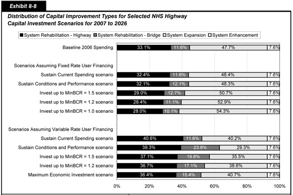
Exhibit 8-8 compares the distribution of highway and bridge capital outlay among the 20-year NHS capital investment scenarios defined in Exhibits 8-6 and 8-7. The amounts identified as the bridge portion of the System Rehabilitation category correspond to the NBIAS-modeled portion of each scenario, while System Enhancement spending corresponds to the non-modeled portion of each scenario as estimated in Exhibits 8-6 and 8-7. The HERS-modeled portion of each scenario is split between the System Expansion category and the highway portion of the System Rehabilitation category.
| Scenario Name and Description | Average Annual Investment (Billions of 2006 Dollars) | |||||
|---|---|---|---|---|---|---|
| System Rehabilitation Highway 1 |
System Rehabilitation Bridge 2 |
System Rehabilitation Total |
System Expansion 3 | System Enhancement | Total | |
| Baseline 2006 Spending | $12.3 | $4.3 | $16.6 | $17.7 | $2.8 | $37.1 |
| Scenarios Assuming Fixed Rate User Financing | ||||||
| Sustain Current Spending scenario | $12.0 | $4.3 | $16.3 | $17.9 | $2.8 | $37.1 |
| Sustain Conditions and Performance scenario | $12.4 | $4.7 | $17.1 | $18.7 | $2.9 | $38.7 |
| Invest up to MinBCR=1.5 scenario | $17.6 | $7.7 | $25.3 | $30.8 | $4.6 | $60.7 |
| Invest up to MinBCR=1.2 scenario | $19.7 | $7.7 | $27.4 | $36.6 | $5.2 | $69.2 |
| Invest up to MinBCR=1.0 scenario | $21.3 | $7.7 | $29.0 | $41.3 | $5.8 | $76.1 |
| Scenarios Assuming Variable Rate User Financing | ||||||
| Sustain Current Spending scenario | $15.1 | $4.3 | $19.4 | $14.9 | $2.8 | $37.1 |
| Sustain Conditions and Performance scenario | $7.7 | $4.7 | $12.4 | $5.8 | $1.5 | $19.6 |
| Invest up to MinBCR=1.5 scenario | $14.4 | $7.7 | $22.1 | $13.8 | $2.9 | $38.9 |
| Invest up to MinBCR=1.2 scenario | $16.5 | $7.7 | $24.2 | $17.3 | $3.4 | $44.9 |
| Maximum Economic Investment scenario (MinBCR=1.0) | $18.2 | $7.7 | $25.9 | $20.4 | $3.8 | $50.1 |
For the versions of the scenarios assuming fixed rate user financing, the percentage of capital investment devoted to system expansion rises as the average annual investment level rises. While 47.7 percent of combined public and private capital investment on the NHS was devoted to System Expansion in 2006, the NHS Sustain Current Spending scenario suggests this percentage should be increased to 48.4 percent, were this level of investment to be sustained over 20 years in constant dollar terms. This suggests that the current performance of the NHS is better in terms of physical conditions than in terms of operational performance. If investment were to rise to the NHS Sustain Conditions and Performance scenario level, the analysis suggests that 48.3 percent of NHS capital investment be directed to System Expansion; the NHS MinBCR=1.0 scenario would direct 54.3 percent of capital investment towards System Expansion. These findings suggest that there are a substantial opportunities for potentially cost-beneficial investments in NHS System Expansion if sufficient funding were available to implement them, but that many of these investments have relatively low benefit-cost ratios, due to the large construction costs associated with these types of investments.
For the versions of the scenarios assuming variable rate user financing, the share of capital investment devoted to System Expansion would rise as the average annual investment level rises, but would remain well below the baseline 2006 value of 47.7 percent. As discussed in Chapter 7, variable congestion pricing would tend to reduce VMT growth in the peak period, thus reducing the need to take widening actions to accommodate the growth. If investment were to decline in constant dollar terms to the NHS Sustain Conditions and Performance scenario level, the analysis suggests that 29.3 percent of NHS capital investment be directed to System Expansion; this share would rise to 40.7 percent for the NHS Maximum Economic Investment scenario. These findings suggest that the widespread adoption of congestion pricing strategies would reduce the relative attractiveness of System Expansion relative to System Rehabilitation, though there would still be opportunities for potentially cost-beneficial investments of all kinds.
Investment Scenario Impacts
Exhibit 8-9 summarizes the potential impacts of the 20-year NHS capital investment scenarios defined in Exhibits 8-6 and 8-7, on selected measures of system conditions and performance. The NHS Sustain Conditions and Performance scenario would by definition be associated with a 0.0 percent change in adjusted average user costs and the bridge investment backlog, as the scenario is designed to represent a level of investment that could allow the 2026 values for these indicators to match their base year 2006 values. For the version of this scenario that assumes fixed rate user financing, average delay per VMT is projected to increase by 5.1 percent, while average pavement roughness (as measured by IRI as defined in Chapter 3) would decline by 1.2 percent. This suggests a tradeoff between improved physical conditions and a worsening of operational performance. The opposite is true for the version of this scenario assuming variable rate user financing, under which average delay per VMT is projected to decrease by 11.4 percent while average IRI increases by 17.7 percent. This suggests that the operational performance improvements associated with the widespread adoption of congestion pricing would be sufficient to allow a significant reduction in NHS capital spending while still having the same net impact on the costs experienced by highway users.
| Scenario Name and Description | Average Annual Investment (Billions of 2006 Dollars) | Percent Change in: Adjusted Average User Costs 1 |
Percent Change in: Average Delay Per VMT 2 |
Percent Change in: Average IRI 3 |
Percent Change in: Bridge Investment Backlog 4 |
|---|---|---|---|---|---|
| Scenarios Assuming Fixed Rate User Financing | |||||
| Sustain Current Spending scenario | $37.1 | 0.3% | 6.7% | 1.1% | 12.8% |
| Sustain Conditions and Performance scenario | $38.7 | 0.0% | 5.1% | -1.2% | 0.0% |
| Invest up to MinBCR=1.5 scenario | $60.7 | -3.6% | -16.8% | -23.4% | -100.0% |
| Invest up to MinBCR=1.2 scenario | $69.2 | -4.7% | -24.3% | -29.0% | -100.0% |
| Invest up to MinBCR=1.0 scenario | $76.1 | -5.4% | -29.8% | -33.2% | -100.0% |
| Scenarios Assuming Variable Rate User Financing | |||||
| Sustain Current Spending scenario | $37.1 | -4.0% | -27.9% | -18.3% | 12.8% |
| Sustain Conditions and Performance scenario | $19.6 | 0.0% | -11.4% | 17.7% | 0.0% |
| Invest up to MinBCR=1.5 scenario | $38.9 | -3.8% | -26.4% | -16.2% | -100.0% |
| Invest up to MinBCR=1.2 scenario | $44.9 | -4.6% | -30.9% | -23.1% | -100.0% |
| Maximum Economic Investment scenario (MinBCR=1.0) | $50.1 | -5.2% | -34.0% | -27.8% | -100.0% |
Relative to the scenario focusing on sustaining current conditions and performance, those scenarios with higher average annual levels of investment would be expected to result in overall improvements to the system, as measured by their impacts on adjusted average user costs and other performance indicators. The potential for reductions to average delay per VMT is relatively large, as strategic investments in NHS System Expansion, coupled with the continued deployment of ITS on a growing share of the NHS, has the potential to significantly improve operating performance, particularly when applied in conjunction with congestion pricing.
It should be noted that while the variable rate user financing version of the Sustain Conditions and Performance scenario is projected to result in higher average IRI than the fixed rate version of the scenario, this is largely attributable to its much lower level of investment. As the Sustain Current Spending scenario demonstrates, given a fixed budget level, variable rate user financing would tend to result in lower average IRI than would fixed rate user financing.
Comparison of Scenario Investment Levels With Base Year Spending
Exhibit 8-10 compares the combined public and private capital investment levels associated with each of the selected NHS scenarios with actual NHS capital spending in 2006. By definition, the NHS Sustain Current Spending scenario matches base year spending in constant dollar terms.
| Scenario Name and Description | Average Annual Investment (Billions of 2006 Dollars) | Difference Relative to 2006 Spending on the NHS (Billions of 2006 Dollars) |
Difference Relative to 2006 Spending on the NHS Percent |
Annual Percent Increase to Support Scenario Investment 1 | Annual Revenues Generated From Variable Rate User Charges 2 |
|---|---|---|---|---|---|
| Scenarios Assuming Fixed Rate User Financing | |||||
| Sustain Current Spending scenario | $37.1 | $0.0 | 0.0% | 0.00% | $0.0 |
| Sustain Conditions and Performance scenario | $38.7 | $1.6 | 4.4% | 0.41% | $0.0 |
| Invest up to MinBCR=1.5 scenario | $60.7 | $23.6 | 63.7% | 4.49% | $0.0 |
| Invest up to MinBCR=1.2 scenario | $69.2 | $32.1 | 86.5% | 5.62% | $0.0 |
| Invest up to MinBCR=1.0 scenario | $76.1 | $39.0 | 105.1% | 6.43% | $0.0 |
| Scenarios Assuming Variable Rate User Financing | |||||
| Sustain Current Spending scenario | $37.1 | $0.0 | 0.0% | 0.00% | $33.9 |
| Sustain Conditions and Performance scenario | $19.6 | -$17.4 | -47.0% | -6.54% | $42.9 |
| Invest up to MinBCR=1.5 scenario | $38.9 | $1.8 | 4.9% | 0.46% | $34.7 |
| Invest up to MinBCR=1.2 scenario | $44.9 | $7.9 | 21.2% | 1.8% | $32.0 |
| Maximum Economic Investment scenario (MinBCR=1.0) | $50.1 | $13.1 | 35.3% | 2.79% | $30.0 |
Among the versions of the scenarios assuming fixed rate user financing, the difference in average annual investment levels relative to the 2006 baseline ranges from 4.4 percent for the NHS Sustain Conditions and Performance scenario up to 105.1 percent for the NHS MinBCR=1.0 scenario. Exhibit 8-10 also identifies the annual increase in combined public and private capital investment that would be sufficient to produce the average annual investment levels identified for each scenario. A constant dollar spending growth rate of 0.41 percent would be sufficient to support the NHS Sustain Conditions and Performance scenario; the equivalent growth rate associated with the NHS MinBCR=1.5 scenario would be 4.49 percent.
Among the versions of the scenarios assuming fixed rate user financing, the average annual investment level for the NHS Sustain Conditions and Performance scenario is 47.0 percent lower than actual NHS capital spending in 2006; Exhibit 8-10 indicates that highway capital spending could decline by 6.54 percent annually in constant dollar terms and still generate sufficient funding to support this scenario. The average annual investment level for the NHS Maximum Economic Investment scenario exceeds base year 2006 NHS capital spending by 35.3 percent. Achieving this average annual investment level could be accomplished by increasing combined public and private NHS capital spending by 2.79 percent per year.
Exhibit 8-10 also identifies the estimated annual revenues that might be generated from the NHS assuming the widespread adoption of congestion pricing. These revenues are a subset of the projected revenue from variable rate user charges identified in Chapter 7 for the highway system as a whole [see Exhibit 7-4]. Based on the assumptions underlying the analyses presented in these scenarios, the additional revenues generated from congestion charges on the NHS would be more than adequate to support an increase in NHS spending up to the NHS Maximum Economic Investment scenario if these revenues were used for this purpose.
Systemwide Scenarios
Exhibits 8-11 and 8-12 describe the derivation of the investment levels for each of five systemwide capital investment scenarios assuming fixed rate user financing and variable rate user financing, respectively. For each of these scenarios, the HERS and NBIAS components can be linked back to one of the 24 alternative funding levels analyzed in Chapter 7. The HERS-derived scenario components link back to selected investment levels identified in Exhibit 7-5, along with the minimum benefit-cost ratio cutoff points identified in Exhibit 7-14. The NBIAS-derived scenario components tie back to selected investment levels identified in Exhibit 7-21. Each scenario covers the 20-year period from 2007 to 2026, and the investment levels shown are all stated in constant 2006 dollars.
Exhibits 8-11 and 8-12 identify the systemwide constant dollar growth rate associated with each of the investment scenario components to provide a link back to the analysis of the potential impacts of these funding levels presented in various exhibits in Chapter 7. By definition, the Sustain Current Spending scenario is associated with annual growth rates of 0.0 percent for all of its components. The Sustain Conditions and Performance scenario is associated with an annual growth rate of 0.83 percent for its NBIAS component; the equivalent growth rates for its HERS component are 3.07 percent assuming fixed rate user financing or -1.37 percent assuming variable rate user financing.
The NBIAS component for the MinBCR=1.5, MinBCR=1.2, and MinBCR=1.0 scenarios is associated with an annual constant dollar growth rate of 5.15 percent for its NBIAS component. Assuming fixed rate user financing, the annual growth rates associated with HERS components of these three scenarios are 5.03 percent, 6.41 percent, and 7.45 percent, respectively; the comparable growth rates assuming variable rate user financing are 1.67 percent, 3.30 percent, and 4.45 percent, respectively.
| What are the minimum benefit-cost ratios associated with the HERS components each of the systemwide scenarios? | |
|
The systemwide annual spending growth rates identified in Exhibits 8-11 and 8-12 are included to provide a link to the performance indicators associated with those growth rates presented in various exhibits in Chapter 7. Exhibit 7-14 indicates that the HERS minimum benefit-cost ratios associated with the 0.0 percent growth rate associated with the Sustain Current Spending Scenario are 2.89 for the fixed rate user financing version and 1.90 assuming variable rate user financing.
For the Sustain Conditions and Performance scenario, the 3.07 percent annual spending growth rate associated with the HERS component of the fixed rate user financing version is linked to a minimum benefit-cost ratio of 1.98. The 1.37 percent annual spending decrease associated with the HERS component of the variable rate user financing version of this scenario is linked to a minimum BCR of 2.25.
By definition, the minimum benefit-cost ratios associated with the MinBCR=1.5 scenario, the MinBCR=1.2 scenario, and the MinBCR=1.0 scenario are 1.5, 1.2, and 1.0, respectively.
|
|
The discussion that follows documents the derivation of the six investment scenarios in some detail. This information is provided to serve as a roadmap for how one could construct additional scenarios building off of different inputs from Chapter 7 beyond the selected scenarios presented here. It is important to note that these scenarios are intended to be illustrative, and any number of alternative scenarios based on different benefit-cost ratio cutoff points, performance targets, or funding targets could be constructed that would be equally valid from a technical perspective.
Derivation of Scenario Investment Levels
The average annual investment levels shown for the Sustain Current Spending scenario are identical in both Exhibits 8-11 and 8-12, and are consistent with the 2006 spending figures identified in Exhibit 7-1. This scenario assumes the continuation of the percentage splits in spending among HERS-modeled, NBIAS-modeled, and non-modeled improvement types. Of the $78.7 billion of highway capital investment by all levels of government in 2006, approximately $48.2 billion (or 61.3 percent) was used for types of improvements modeled in HERS, including pavement resurfacing, pavement reconstruction, and capacity additions to the existing highway and bridge network. Approximately $10.1 billion (or 12.9 percent) was used for types of bridge repair, rehabilitation, and replacement improvements modeled in NBIAS. The remaining $20.3 billion (or 25.9 percent) went for types of capital improvements not currently addressed by either HERS or NBIAS ($8.2 billion), including various safety enhancements, environmental enhancements, and traffic operations improvements or for highway functional systems not reported in the Highway Performance Monitoring System ($12.1 billion), including roads functionally classified as rural minor collector, rural local, or urban local.
| Scenario Name and Description | Scenario Component (And Associated Systemwide Growth Rate) * | Share of 2006 Total Capital Outlay | Average Annual Investment (Billions of 2006 Dollars) Modeled Spending |
Average Annual Investment (Billions of 2006 Dollars) Estimated Non-Modeled |
Average Annual Investment (Billions of 2006 Dollars) Total |
Share of Average Annual Investment |
|---|---|---|---|---|---|---|
| Sustain Current Spending scenario (Maintain spending at base year levels in constant dollar terms) |
HERS (0.00%) | 61.3% | $48.2 | $48.2 | 61.3% | |
| Sustain Current Spending scenario (Maintain spending at base year levels in constant dollar terms) |
NBIAS (0.00%) | 12.9% | $10.1 | $10.0 | 12.9% | |
| Sustain Current Spending scenario (Maintain spending at base year levels in constant dollar terms) |
Non-Modeled | 25.9% | $20.3 | $20.3 | 25.9% | |
| Sustain Current Spending scenario (Maintain spending at base year levels in constant dollar terms) |
Total | 100.0% | $58.3 | $20.3 | $78.7 | 100.0% |
| Sustain Conditions and Performance scenario (Maintain adjusted average highway user costs and economic bridge backlog at 2006 levels) |
HERS (3.07%) | 61.3% | $67.2 | $67.2 | 63.7% | |
| Sustain Conditions and Performance scenario (Maintain adjusted average highway user costs and economic bridge backlog at 2006 levels) |
NBIAS (0.83%) | 12.9% | $11.1 | $11.1 | 10.5% | |
| Sustain Conditions and Performance scenario (Maintain adjusted average highway user costs and economic bridge backlog at 2006 levels) |
Non-Modeled | 25.9% | $27.3 | $27.3 | 25.9% | |
| Sustain Conditions and Performance scenario (Maintain adjusted average highway user costs and economic bridge backlog at 2006 levels) |
Total | 100.0% | $78.3 | $27.3 | $105.6 | 100.0% |
| MinBCR=1.5 scenario (Invest in projects with BCRs as low as 1.5 and eliminate economic backlog for bridge rehabilitation) |
HERS (5.03%) | 61.3% | $84.0 | $84.0 | 61.1% | |
| MinBCR=1.5 scenario (Invest in projects with BCRs as low as 1.5 and eliminate economic backlog for bridge rehabilitation) |
NBIAS (5.15%) | 12.9% | $17.9 | $17.9 | 13.0% | |
| MinBCR=1.5 scenario (Invest in projects with BCRs as low as 1.5 and eliminate economic backlog for bridge rehabilitation) |
Non-Modeled | 25.9% | $35.5 | $35.5 | 25.9% | |
| MinBCR=1.5 scenario (Invest in projects with BCRs as low as 1.5 and eliminate economic backlog for bridge rehabilitation) |
Total | 100.0% | $101.9 | $35.5 | $134.4 | 100.0% |
| MinBCR=1.2 scenario (Invest in projects with BCRs as low as 1.2 and eliminate economic backlog for bridge rehabilitation) |
HERS (6.41%) | 61.3% | $98.6 | $98.6 | 62.8% | |
| MinBCR=1.2 scenario (Invest in projects with BCRs as low as 1.2 and eliminate economic backlog for bridge rehabilitation) |
NBIAS (5.15%) | 12.9% | $17.9 | $17.9 | 11.4% | |
| MinBCR=1.2 scenario (Invest in projects with BCRs as low as 1.2 and eliminate economic backlog for bridge rehabilitation) |
Non-Modeled | 25.9% | $40.6 | $40.6 | 25.9% | |
| MinBCR=1.2 scenario (Invest in projects with BCRs as low as 1.2 and eliminate economic backlog for bridge rehabilitation) |
Total | 100.0% | $116.5 | $40.6 | $157.1 | 100.0% |
| Maximum Economic Investment (MinBCR=1.0) scenario (Invest in projects with BCRs as low as 1.0 and eliminate economic bridge backlog) |
HERS (7.45%) | 61.3% | $111.5 | $111.5 | 63.9% | |
| Maximum Economic Investment (MinBCR=1.0) scenario (Invest in projects with BCRs as low as 1.0 and eliminate economic bridge backlog) |
NBIAS (5.15%) | 12.9% | $17.9 | $17.9 | 10.2% | |
| Maximum Economic Investment (MinBCR=1.0) scenario (Invest in projects with BCRs as low as 1.0 and eliminate economic bridge backlog) |
Non-Modeled | 25.9% | $45.1 | $45.1 | 25.9% | |
| Maximum Economic Investment (MinBCR=1.0) scenario (Invest in projects with BCRs as low as 1.0 and eliminate economic bridge backlog) |
Total | 100.0% | $129.4 | $45.1 | $174.6 | 100.0% |
| Scenario Name and Description | Scenario Component (And Associated Systemwide Growth Rate) * | Share of 2006 Total Capital Outlay | Average Annual Investment (Billions of 2006 Dollars) Modeled Spending |
Average Annual Investment (Billions of 2006 Dollars) Estimated Non-Modeled |
Average Annual Investment (Billions of 2006 Dollars) Total |
Share of Average Annual Investment |
|---|---|---|---|---|---|---|
| Sustain Current Spending scenario (Maintain spending at base year levels in constant dollar terms) |
HERS (0.00%) | 61.3% | $48.2 | $48.2 | 61.3% | |
| Sustain Current Spending scenario (Maintain spending at base year levels in constant dollar terms) |
NBIAS (0.00%) | 12.9% | $10.1 | $10.1 | 112.9% | |
| Sustain Current Spending scenario (Maintain spending at base year levels in constant dollar terms) |
Non-Modeled | 25.9% | $20.3 | $20.3 | 25.9% | |
| Sustain Current Spending scenario (Maintain spending at base year levels in constant dollar terms) |
Total | 100.0% | $58.3 | $20.3 | $78.7 | 100.0% |
| Sustain Conditions and Performance scenario (Maintain adjusted average highway user costs and economic bridge backlog at 2006 levels) |
HERS (-1.37%) | 61.3% | $41.8 | $41.8 | 58.6% | |
| Sustain Conditions and Performance scenario (Maintain adjusted average highway user costs and economic bridge backlog at base year levels) |
NBIAS (0.83%) | 12.9% | $11.1 | $11.1 | 15.5% | |
| Sustain Conditions and Performance scenario (Maintain adjusted average highway user costs and economic bridge backlog at base year levels) |
Non-Modeled | 25.9% | $18.4 | $18.4 | 25.9% | |
| Sustain Conditions and Performance scenario (Maintain adjusted average highway user costs and economic bridge backlog at base year levels) |
Total | 100.0% | $52.9 | $18.4 | $71.3 | 100.0% |
| MinBCR=1.5 scenario (Invest in projects with BCRs as low as 1.5 and eliminate economic backlog for bridge rehabilitation) |
HERS (1.67%) | 61.3% | $57.6 | $57.6 | 56.6% | |
| MinBCR=1.5 scenario (Invest in projects with BCRs as low as 1.5 and eliminate economic backlog for bridge rehabilitation) |
NBIAS (5.15%) | 12.9% | $17.9 | $17.9 | 17.6% | |
| MinBCR=1.5 scenario (Invest in projects with BCRs as low as 1.5 and eliminate economic backlog for bridge rehabilitation) |
Non-Modeled | 25.9% | $26.3 | $26.3 | 25.9% | |
| MinBCR=1.5 scenario (Invest in projects with BCRs as low as 1.5 and eliminate economic backlog for bridge rehabilitation) |
Total | 100.0% | $75.5 | $26.3 | $101.8 | 100.0% |
| MinBCR=1.2 scenario (Invest in projects with BCRs as low as 1.2 and eliminate economic backlog for bridge rehabilitation) |
HERS (3.30%) | 61.3% | $69.0 | $69.0 | 58.9% | |
| MinBCR=1.2 scenario (Invest in projects with BCRs as low as 1.2 and eliminate economic backlog for bridge rehabilitation) |
NBIAS (5.15%) | 12.9% | $17.9 | $17.9 | 15.3% | |
| MinBCR=1.2 scenario (Invest in projects with BCRs as low as 1.2 and eliminate economic backlog for bridge rehabilitation) |
Non-Modeled | 25.9% | $30.3 | $30.3 | 25.9% | |
| MinBCR=1.2 scenario (Invest in projects with BCRs as low as 1.2 and eliminate economic backlog for bridge rehabilitation) |
Total | 100.0% | $86.9 | $30.3 | $117.2 | 100.0% |
| Maximum Economic Investment (MinBCR=1.0) scenario (Invest in projects with BCRs as low as 1.0 and eliminate economic bridge backlog) |
HERS (4.45%) | 61.3% | $79.5 | $79.5 | 60.5% | |
| Maximum Economic Investment (MinBCR=1.0) scenario (Invest in projects with BCRs as low as 1.0 and eliminate economic bridge backlog) |
NBIAS (5.15%) | 12.9% | $17.9 | $17.9 | 13.6% | |
| Maximum Economic Investment (MinBCR=1.0) scenario (Invest in projects with BCRs as low as 1.0 and eliminate economic bridge backlog) |
Non-Modeled | 25.9% | $34.0 | $34.0 | 25.9% | |
| Maximum Economic Investment (MinBCR=1.0) scenario (Invest in projects with BCRs as low as 1.0 and eliminate economic bridge backlog) |
Total | 100.0% | $97.4 | $34.0 | $131.3 | 100.0% |
Each of the investment scenarios assume that the share of average annual investment directed towards non-modeled capital improvements will remain at the 2006 level of 25.9 percent. Consequently, the amounts identified as estimated non-modeled spending in Exhibits 8-11 and 8-12 are proportionally larger or smaller than the 2006 spending level of $20.3 billion, based on the change in modeled spending relative to the 2006 baseline.
The average annual investment level for the Sustain Conditions and Performance scenario for 2007 to 2026 assuming fixed rate user financing is $105.6 billion, as shown in Exhibit 8-11, while Exhibit 8-12 identifies the comparable annual figure assuming the widespread adoption of variable rate user charges (i.e., congestion pricing) as $71.3 billion in constant 2006 dollars. The HERS-modeled components of these totals are $67.2 billion and $41.8 billion, respectively. The NBIAS modeled component is identical in both exhibits, totaling $11.1 billion, as NBIAS does not consider alternative financing mechanisms. The estimated non-modeled portion of the scenario differs proportionally in response to the differences between the HERS-derived figures.
As shown in Exhibit 8-11, the average annual investment level for the period 2007 to 2026 for the MinBCR=1.5 scenario assuming financing from fixed rate user charges is $137.4 billion, including a HERS-derived component of $84.0 billion, stated in constant 2006 dollars. Exhibit 8-12 identifies an average annual investment for the MinBCR=1.5 scenario of $101.8 billion stated in constant 2006 dollars assuming financing from variable rate user charges, including a HERS-derived component of $57.6 billion. The $17.9 billion NBIAS-derived component shown in both Exhibits 8-11 and 8-12 represents the average annual level of investment to eliminate the economic bridge investment backlog.
The average annual investment level over 20 years for the MinBCR=1.2 scenario assuming financing from fixed rate user charges is $157.1 billion stated in constant 2006 dollars, including a HERS-derived component of $98.6 billion, as shown in Exhibit 8-11. Exhibit 8-12 identifies an average annual investment for the MinBCR=1.2 scenario of $117.2 billion stated in constant 2006 dollars assuming financing from variable rate user charges, including a HERS-derived component of $69.0 billion. The $17.9 billion NBIAS-derived component shown in both Exhibits 8-11 and 8-12 represents the average annual level of investment to eliminate the economic bridge investment backlog.
The average annual investment level over 20 years for the MinBCR=1.0 scenario assuming financing from fixed rate user charges is $174.6 billion stated in constant 2006 dollars, including a HERS-derived component of $111.5 billion, as shown in Exhibit 8-11. Exhibit 8-12 identifies an average annual investment for the Maximum Economic Investment (MinBCR=1.0) scenario of $131.3 billion stated in constant 2006 dollars assuming the widespread adoption of variable user charges such as congestion pricing, including a HERS-derived component of $79.5 billion. The $17.9 billion NBIAS-derived component shown in both Exhibits 8-11 and 8-12 represents the average annual level of investment to eliminate the economic bridge investment backlog.
Investment Scenario Estimates by Improvement Type
Exhibit 8-13 compares the distribution of highway and bridge capital spending by type of improvement among the 20-year capital investment scenarios defined in Exhibits 8-11 and 8-12. The amounts identified as the bridge portion of the System Rehabilitation category correspond to the NBIAS-modeled portion of each scenario. Amounts identified as System Enhancement spending represent a subset of the non-modeled portion of each scenario as estimated in Exhibits 8-11 and 8-12; the remaining non-modeled spending and the HERS-modeled portion of each scenario are split between the System Expansion category and the highway portion of the System Rehabilitation category.
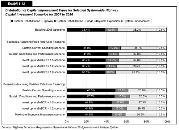
For the versions of the scenarios assuming fixed rate user financing, the percentage of capital investment devoted to System Expansion generally rises as the average annual investment level rises. While 38.2 percent of combined public and private highway capital investment was devoted to System Expansion in 2006, the Sustain Current Spending scenario suggests this percentage be decreased to 35.7 percent, were this level of investment to be sustained over 20 years in constant dollar terms. If investment were to rise to the MinBCR=1.0 level, the analysis suggests that 40.7 percent of capital investment be directed to System Expansion.
For the versions of the scenarios assuming variable rate user financing, the percentage of capital investment devoted to system expansion would be lower than if only fixed rate user financing were utilized, but would still generally rise as the average annual investment level rises. If investment were to decline in constant dollar terms to the Sustain Conditions and Performance scenario level, the analysis suggests that 26.3 percent of capital investment be directed to System Expansion; this share would rise to 28.0 percent for the Sustain Current Spending scenario, and to 30.9 percent if investment were to rise to the Maximum Economic Investment scenario level. These findings suggest that the widespread adoption of congestion pricing strategies would reduce the relative attractiveness of System Expansion relative to System Rehabilitation, though there would still be plentiful opportunities for potentially cost-beneficial investments of all kinds.
Sustain Current Spending Scenario
Exhibits 8-14 and 8-15 identify the distribution of capital investments for the Sustain Current Spending scenario (assuming fixed rate financing and variable rate financing, respectively) with the actual distribution of highway capital spending by all levels of government in 2006. In assessing the percentage differences shown in this table, it is important to note that the distribution of expenditures tends to vary from year to year, and that 2006 does not necessarily represent a typical year in regards to spending for each of the capital improvement types on each functional class identified in the exhibits; in some cases, this may make the relative differences between the scenario and current spending patterns appear more dramatic than they actually are. In both exhibits, for all functional classes, the percent differences shown in the "System Enhancement" column are 0.0 percent, as these types of improvements are not modeled and were assumed to remain constant; the same is true for the rural minor collector and local functional class values in the "System Expansion" and "System Rehabilitation: Highway" columns.
| Average Annual National Investment (Billions of 2006 Dollars) | ||||||
|---|---|---|---|---|---|---|
| Functional Class | System Rehabilitation Highway |
System Rehabilitation Bridge |
System Rehabilitation Total |
System Expansion | System Enhancement | Total |
| Rural Arterials and Collectors | ||||||
| Interstate | $1.6 | $0.6 | $2.1 | $1.8 | $0.4 | $4.3 |
| Other Principal Arterial | $1.2 | $0.5 | $1.7 | $0.8 | $0.6 | $3.1 |
| Minor Arterial | $1.1 | $0.4 | $1.5 | $0.2 | $0.5 | $2.2 |
| Major Collector | $1.6 | $0.7 | $2.3 | $0.2 | $0.4 | $2.9 |
| Minor Collector | $0.6 | $0.3 | $0.8 | $0.2 | $0.1 | $1.2 |
| Subtotal | $6.0 | $2.5 | $8.5 | $3.2 | $2.0 | $13.7 |
| Urban Arterials and Collectors | ||||||
| Interstate | $5.7 | $2.3 | $8.0 | $10.9 | $0.9 | $19.8 |
| Other Freeway and Expressway | $2.4 | $0.9 | $3.3 | $3.7 | $0.4 | $7.5 |
| Other Principal Arterial | $4.2 | $1.5 | $5.8 | $2.6 | $1.0 | $9.4 |
| Minor Arterial | $5.0 | $1.2 | $6.2 | $2.5 | $0.7 | $9.4 |
| Collector | $1.8 | $0.4 | $2.2 | $0.9 | $0.4 | $3.6 |
| Subtotal | $19.1 | $6.4 | $25.5 | $20.6 | $3.5 | $49.7 |
| Rural and Urban Local | $7.1 | $1.3 | $8.4 | $4.2 | $2.7 | $15.4 |
| Total | $32.2 | $10.1 | $42.4 | $28.1 | $8.2 | $78.7 |
| Percent Above Actual 2006 Combined Public and Private Capital Spending | ||||||
| Rural Arterials and Collectors | ||||||
| Interstate | -38.8% | 71.9% | -25.8% | 84.4% | 0.0% | 1.8% |
| Other Principal Arterial | -66.9% | -34.9% | -61.5% | -83.3% | 0.0% | -68.0% |
| Minor Arterial | -52.5% | -44.0% | -50.4% | -83.2% | 0.0% | -54.7% |
| Major Collector | -34.8% | -13.4% | -29.4% | -68.7% | 0.0% | -33.3% |
| Minor Collector | 0.0% | -18.6% | -6.7% | 0.0% | 0.0% | -4.9% |
| Subtotal | -47.6% | -17.7% | -41.4% | -59.3% | 0.0% | -43.8% |
| Urban Arterials and Collectors | ||||||
| Interstate | 77.3% | 6.8% | 49.0% | 79.7% | 0.0% | 60.6% |
| Other Freeway and Expressway | 71.0% | 90.8% | 75.9% | 17.7% | 0.0% | 36.3% |
| Other Principal Arterial | 26.4% | 66.0% | 34.9% | -51.2% | 0.0% | -11.5% |
| Minor Arterial | 114.2% | 38.7% | 93.5% | 1.5% | 0.0% | 47.5% |
| Collector | 27.1% | -14.0% | 16.4% | -5.1% | 0.0% | 7.8% |
| Subtotal | 63.3% | 29.5% | 53.3% | 15.0% | 0.0% | 30.3% |
| Rural and Urban Local | 0.0% | -41.5% | -9.8% | 0.0% | 0.0% | -5.6% |
| Total | 6.5% | 0.0% | 4.9% | -6.6% | 0.0% | 0.0% |
| Average Annual National Investment (Billions of 2006 Dollars) | ||||||
|---|---|---|---|---|---|---|
| Functional Class | System Rehabilitation Highway |
System Rehabilitation Bridge |
System Rehabilitation Total |
System Expansion | System Enhancement | Total |
| Rural Arterials and Collectors | ||||||
| Interstate | $1.9 | $0.6 | $2.5 | $1.7 | $0.4 | $4.6 |
| Other Principal Arterial | $1.8 | $0.5 | $2.3 | $1.0 | $0.6 | $3.9 |
| Minor Arterial | $1.8 | $0.4 | $2.3 | $0.3 | $0.5 | $3.0 |
| Major Collector | $2.7 | $0.7 | $3.4 | $0.3 | $0.4 | $4.1 |
| Minor Collector | $0.6 | $0.3 | $0.8 | $0.2 | $0.1 | $1.2 |
| Subtotal | $8.9 | $2.5 | $11.3 | $3.5 | $2.0 | $16.8 |
| Urban Arterials and Collectors | ||||||
| Interstate | $5.2 | $2.3 | $7.5 | $6.1 | $0.9 | $14.4 |
| Other Freeway and Expressway | $2.4 | $0.9 | $3.3 | $2.1 | $0.4 | $5.8 |
| Other Principal Arterial | $5.5 | $1.5 | $7.0 | $2.4 | $1.0 | $10.5 |
| Minor Arterial | $6.5 | $1.2 | $7.7 | $2.7 | $0.7 | $11.1 |
| Collector | $2.8 | $0.4 | $3.2 | $1.0 | $0.4 | $4.7 |
| Subtotal | $22.3 | $6.4 | $28.7 | $14.3 | $3.5 | $46.5 |
| Rural and Urban Local | $7.1 | $1.3 | $8.4 | $4.2 | $2.7 | $15.4 |
| Total | $38.3 | $10.1 | $48.4 | $22.0 | $8.2 | $78.7 |
| Percent Above Actual 2006 Combined Public and Private Capital Spending | ||||||
| Rural Arterials and Collectors | ||||||
| Interstate | -24.4% | 71.9% | -13.1% | 75.5% | 0.0% | 81.8% |
| Other Principal Arterial | -49.0% | -34.9% | -46.6% | -79.0% | 0.0% | -59.1% |
| Minor Arterial | -20.4% | -44.0% | -26.4% | -79.7% | 0.0% | -38.6% |
| Major Collector | 11.8% | -13.4% | 5.4% | -56.8% | 0.0% | -5.7% |
| Minor Collector | 0.0% | -18.6% | -6.7% | 0.0% | 0.0% | -4.9% |
| Subtotal | -22.5% | -17.7% | -21.5% | -55.9% | 0.0% | -30.9% |
| Urban Arterials and Collectors | ||||||
| Interstate | 60.0% | 6.8% | 38.6% | -0.1% | 0.0% | 16.8% |
| Other Freeway and Expressway | 67.2% | 90.8% | 73.1% | -33.7% | 0.0% | 5.7% |
| Other Principal Arterial | 63.9% | 66.0% | 64.3% | -54.7% | 0.0% | -1.4% |
| Minor Arterial | 178.5% | 38.7% | 140.2% | 12.2% | 0.0% | 75.1% |
| Collector | 100.5% | -14.0% | 70.6% | 5.6% | 0.0% | 42.2% |
| Subtotal | 90.3% | 29.5% | 72.3% | -20.1% | 0.0% | 22.1% |
| Rural and Urban Local | 0.0% | -41.5% | -9.8% | 0.0% | 0.0% | -5.6% |
| Total | 26.5% | 0.0% | 19.8% | -26.6% | 0.0% | 0.0% |
The HERS and NBIAS analyses underlying the distribution of capital investments shown in Exhibit 8-14 suggest that if combined public and private highway capital spending were maintained at base year 2006 levels in constant dollar terms and fixed rate user financing mechanisms were utilized, then shifting resources from rural arterials and collectors to urban arterials and collectors would yield a more favorable outcome in terms of total net benefits to users, agencies, and society. The $13.7 billion of combined public and private investment on rural arterials and collectors included as part of this scenario would represent a 43.8 percent decline relative to actual 2006 spending. The scenario does include a 1.8 percent increase in capital spending on rural interstates relative to the 2006 baseline, as HERS and NBIAS identified a relatively large pool of attractive investments in Interstate System Expansion and Interstate Bridge Rehabilitation. The $49.7 billion of combined investment on urban arterials and collectors included as part of this scenario would represent a 30.3 percent increase relative to actual spending.
Exhibit 8-15 shows that assuming the widespread adoption of variable rate user financing mechanisms such as congestion pricing would make some potential urban capital investments less economically attractive than those in rural areas. However, the $16.8 billion of capital investment on rural arterials and collectors assumed under this scenario would represent a 30.9 percent decrease relative to the 2006 baseline; the $46.5 billion of capital investment on urban arterials and collectors would represent a 22.1 percent increase. The HERS and NBIAS analyses underlying the distribution of capital investments shown in Exhibit 8-15 suggest shifting significant resources towards urban system rehabilitation.
Sustain Conditions and Performance Scenario
Exhibit 8-16 identifies the distribution of capital investments by improvement type and functional class for the Sustain Conditions and Performance scenario. Assuming fixed rate user financing, the $67.2 billion of capital investment on urban arterials and collectors under this scenario would represent 63.7 percent of the $105.6 billion total public and private average annual capital spending under this scenario. Investment on rural arterials collectors under this scenario totals $18.1 billion (17.1 percent), while the rural and urban local roads and streets component totals $20.3 billion (19.2 percent).
| Assuming Fixed Rate User Financing | ||||||
|---|---|---|---|---|---|---|
| Functional Class | System Rehabilitation Highway |
System Rehabilitation Bridge |
System Rehabilitation Total |
System Expansion | System Enhancement | Total |
| Rural Arterials and Collectors | ||||||
| Interstate | $2.0 | $0.6 | $2.6 | $2.1 | $0.5 | $5.2 |
| Other Principal Arterial | $1.8 | $0.5 | $2.3 | $1.0 | $0.8 | $4.1 |
| Minor Arterial | $1.7 | $0.5 | $2.2 | $0.3 | $0.6 | $3.1 |
| Major Collector | $2.5 | $0.7 | $3.2 | $0.3 | $0.6 | $4.1 |
| Minor Collector | $0.8 | $0.3 | $1.1 | $0.2 | $0.1 | $1.5 |
| Subtotal | $8.7 | $2.6 | $11.4 | $4.0 | $2.7 | $18.1 |
| Urban Arterials and Collectors | ||||||
| Interstate | $7.1 | $2.5 | $9.5 | $15.0 | $1.2 | $25.7 |
| Other Freeway and Expressway | $3.0 | $1.0 | $4.0 | $5.7 | $0.6 | $10.3 |
| Other Principal Arterial | $5.8 | $1.7 | $7.5 | $4.3 | $1.4 | $13.2 |
| Minor Arterial | $6.6 | $1.4 | $8.0 | $3.7 | $1.0 | $12.6 |
| Collector | $2.8 | $0.5 | $3.3 | $1.7 | $0.6 | $5.5 |
| Subtotal | $25.3 | $7.0 | $32.3 | $30.3 | $4.7 | $67.2 |
| Rural and Urban Local | $9.5 | $1.4 | $10.9 | $5.7 | $5.7 | $20.3 |
| Total | $43.5 | $11.1 | $54.6 | $40.0 | $11.1 | $105.6 |
| Assuming Variable Rate User Financing | ||||||
| Rural Arterials and Collectors | ||||||
| Interstate | $1.7 | $0.6 | $2.4 | $1.5 | $0.3 | $4.2 |
| Other Principal Arterial | $1.5 | $0.5 | $2.0 | $0.9 | $0.6 | $3.5 |
| Minor Arterial | $1.5 | $0.5 | $2.0 | $0.2 | $0.4 | $2.7 |
| Major Collector | $2.2 | $0.7 | $2.9 | $0.2 | $0.4 | $3.6 |
| Minor Collector | $0.5 | $0.3 | $0.8 | $0.2 | $0.1 | $1.0 |
| Subtotal | $7.5 | $2.6 | $10.1 | $3.1 | $1.8 | $15.0 |
| Urban Arterials and Collectors | ||||||
| Interstate | $4.8 | $2.5 | $7.2 | $5.1 | $0.8 | $13.1 |
| Other Freeway and Expressway | $2.2 | $1.0 | $3.2 | $1.8 | $0.4 | $5.3 |
| Other Principal Arterial | $5.0 | $1.7 | $6.6 | $2.1 | $0.9 | $9.6 |
| Minor Arterial | $5.8 | $1.4 | $7.2 | $2.2 | $0.7 | $10.0 |
| Collector | $2.4 | $0.5 | $2.9 | $0.8 | $0.4 | $4.1 |
| Subtotal | $20.1 | $7.0 | $27.1 | $11.9 | $3.2 | $42.1 |
| Rural and Urban Local | $6.4 | $1.4 | $7.9 | $3.8 | $2.5 | $14.2 |
| Total | $34.0 | $11.1 | $45.1 | $18.8 | $7.5 | $71.3 |
Assuming variable rate user financing, the relative share of capital investment devoted to urban arterials and collectors would be lower. The $42.1 billion directed toward urban arterials and collectors under this scenario would represent 59.1 percent of the $71.3 billion average annual capital spending under this scenario, stated in 2006 dollars. Investment on rural arterials and collectors under this scenario totals $15.0 billion (21.0 percent), while the rural and urban local roads and streets component totals $14.2 billion (19.9 percent).
| Do the amounts identified for each functional class in Exhibit 8-16 represent the costs associated with maintaining the conditions and performance of that functional class? | |
|
No. It is important to note that the goal of the Sustain Conditions and Performance scenario is to maintain average conditions and performance on a systemwide basis; the conditions and performance of individual functional classes may vary. Consequently, the dollar amount shown for each functional class does not represent the cost of maintaining the condition or performance of that functional class in isolation.
A supplemental scenario is presented later in this chapter that identifies the costs associated with maintaining the conditions and performance of individual system components.
|
|
MinBCR=1.5 Scenario
Exhibit 8-17 identifies the distribution of capital investments by improvement type and functional class for the MinBCR=1.5 scenario, in which the investment level is determined as the amount that would support potential investments with a benefit-cost ratio of 1.5 or higher. Assuming fixed rate user financing, the $87.5 billion of capital investment on urban arterials and collectors under the MinBCR=1.5 scenario would represent 63.7 percent of the $137.4 billion total public and private average annual capital spending under this scenario. Investment on rural arterials collectors under this scenario totals $23.0 billion (16.7 percent), while the rural and urban local roads and streets component totals $26.9 billion (19.6 percent).
| Assuming Fixed Rate User Financing | ||||||
|---|---|---|---|---|---|---|
| Functional Class | System Rehabilitation Highway |
System Rehabilitation Bridge |
System Rehabilitation Total |
System Expansion | System Enhancement | Total |
| Rural Arterials and Collectors | ||||||
| Interstate | $2.2 | $0.9 | $3.2 | $2.3 | $0.6 | $6.0 |
| Other Principal Arterial | $2.3 | $0.7 | $3.0 | $1.2 | $1.1 | $5.3 |
| Minor Arterial | $2.2 | $0.7 | $2.9 | $0.4 | $0.8 | $4.1 |
| Major Collector | $3.3 | $1.1 | $4.4 | $0.4 | $0.7 | $5.5 |
| Minor Collector | $1.0 | $0.4 | $1.4 | $0.3 | $0.2 | $2.0 |
| Subtotal | $11.1 | $3.7 | $14.8 | $4.7 | $3.5 | $23.0 |
| Urban Arterials and Collectors | ||||||
| Interstate | $8.0 | $3.8 | $11.7 | $18.9 | $1.5 | $32.2 |
| Other Freeway and Expressway | $3.6 | $1.4 | $5.0 | $7.8 | $0.8 | $13.5 |
| Other Principal Arterial | $7.1 | $2.9 | $10.0 | $5.9 | $1.8 | $17.7 |
| Minor Arterial | $7.6 | $2.7 | $10.3 | $5.2 | $1.3 | $16.8 |
| Collector | $3.4 | $1.0 | $4.4 | $2.1 | $0.7 | $7.3 |
| Subtotal | $29.7 | $11.8 | $41.5 | $39.9 | $6.1 | $87.5 |
| Rural and Urban Local | $12.4 | $2.3 | $14.7 | $7.4 | $4.8 | $26.9 |
| Total | $53.2 | $17.9 | $71.0 | $51.9 | $14.1 | $137.4 |
| Assuming Variable Rate User Financing | ||||||
| Rural Arterials and Collectors | ||||||
| Interstate | $2.1 | $0.9 | $3.1 | $2.0 | $0.5 | $5.5 |
| Other Principal Arterial | $2.3 | $0.7 | $3.0 | $1.1 | $0.8 | $5.0 |
| Minor Arterial | $2.2 | $0.7 | $2.9 | $0.3 | $0.6 | $3.9 |
| Major Collector | $3.4 | $1.1 | $4.4 | $0.4 | $0.5 | $5.4 |
| Minor Collector | $0.7 | $0.4 | $1.2 | $0.2 | $0.2 | $1.6 |
| Subtotal | $10.9 | $3.7 | $14.6 | $4.1 | $2.6 | $21.3 |
| Urban Arterials and Collectors | ||||||
| Interstate | $5.9 | $3.8 | $9.6 | $7.6 | $1.1 | $18.4 |
| Other Freeway and Expressway | $2.7 | $1.4 | $4.1 | $2.7 | $0.6 | $7.4 |
| Other Principal Arterial | $6.4 | $2.9 | $9.4 | $3.1 | $1.3 | $13.8 |
| Minor Arterial | $7.2 | $2.7 | $9.9 | $3.3 | $1.0 | $14.2 |
| Collector | $3.4 | $1.0 | $4.4 | $1.3 | $0.5 | $6.2 |
| Subtotal | $25.6 | $11.8 | $37.4 | $18.1 | $4.5 | $60.1 |
| Rural and Urban Local | $9.2 | $2.3 | $11.5 | $5.5 | $3.5 | $20.5 |
| Total | $45.7 | $17.9 | $63.5 | $27.6 | $10.7 | $101.8 |
Assuming variable rate user financing, the relative share of capital investment devoted to urban arterials and collectors would be lower. The $60.1 billion directed toward urban arterials and collectors under this scenario would represent 59.0 percent of the $101.8 billion average annual capital spending under this scenario, stated in 2006 dollars. Investment on rural arterials and collectors under this scenario totals $21.3 billion (20.9 percent), while the rural and urban local roads and streets component totals $20.5 billion (20.2 percent).
MinBCR=1.2 Scenario
Exhibit 8-18 identifies the distribution of capital investments by improvement type and functional class for the MinBCR=1.2 scenario, in which the investment level is determined as the amount that would support potential investments with a benefit-cost ratio of 1.2 or higher. Assuming fixed rate user financing, the $100.4 billion of capital investment on urban arterials and collectors under the MinBCR=1.2 scenario would represent 63.9 percent of the $157.1 billion total public and private average annual capital spending under this scenario. Investment on rural arterials collectors under this scenario totals $26.3 billion (16.8 percent), while the rural and urban local roads and streets component totals $30.4 billion (19.4 percent).
| Assuming Fixed Rate User Financing | ||||||
|---|---|---|---|---|---|---|
| Functional Class | System Rehabilitation Highway |
System Rehabilitation Bridge |
System Rehabilitation Total |
System Expansion | System Enhancement | Total |
| Rural Arterials and Collectors | ||||||
| Interstate | $2.5 | $0.9 | $3.4 | $2.5 | $0.7 | $6.6 |
| Other Principal Arterial | $2.8 | $0.7 | $3.5 | $1.5 | $1.2 | $6.2 |
| Minor Arterial | $2.7 | $0.7 | $3.4 | $0.5 | $0.9 | $4.8 |
| Major Collector | $4.1 | $1.1 | $5.1 | $0.5 | $0.8 | $6.5 |
| Minor Collector | $1.2 | $0.4 | $1.6 | $0.4 | $0.3 | $2.2 |
| Subtotal | $13.3 | $3.7 | $17.0 | $5.3 | $4.0 | $26.3 |
| Urban Arterials and Collectors | ||||||
| Interstate | $8.6 | $3.8 | $12.4 | $22.1 | $1.7 | $36.2 |
| Other Freeway and Expressway | $3.9 | $1.4 | $5.4 | $9.7 | $0.9 | $15.9 |
| Other Principal Arterial | $8.4 | $2.9 | $11.3 | $7.7 | $2.1 | $21.1 |
| Minor Arterial | $8.4 | $2.7 | $11.1 | $6.0 | $1.5 | $18.6 |
| Collector | $4.0 | $1.0 | $5.0 | $2.7 | $0.8 | $8.6 |
| Subtotal | $33.3 | $11.8 | $45.1 | $48.2 | $7.0 | $100.4 |
| Rural and Urban Local | $14.2 | $2.3 | $16.5 | $8.4 | $5.5 | $30.4 |
| Total | $60.8 | $17.9 | $78.7 | $62.0 | $16.5 | $157.1 |
| Assuming Variable Rate User Financing | ||||||
| Rural Arterials and Collectors | ||||||
| Interstate | $2.4 | $0.9 | $3.3 | $2.2 | $0.5 | $6.0 |
| Other Principal Arterial | $2.8 | $0.7 | $3.5 | $1.4 | $0.9 | $5.8 |
| Minor Arterial | $2.8 | $0.7 | $3.5 | $0.5 | $0.7 | $4.6 |
| Major Collector | $4.2 | $1.1 | $5.3 | $0.5 | $0.6 | $6.4 |
| Minor Collector | $0.9 | $0.4 | $1.3 | $0.3 | $0.2 | $1.8 |
| Subtotal | $13.1 | $3.7 | $16.8 | $4.8 | $3.0 | $24.6 |
| Urban Arterials and Collectors | ||||||
| Interstate | $6.6 | $3.8 | $10.4 | $9.6 | $1.3 | $21.3 |
| Other Freeway and Expressway | $3.0 | $1.4 | $4.5 | $3.4 | $0.7 | $8.5 |
| Other Principal Arterial | $7.6 | $2.9 | $10.5 | $4.3 | $1.5 | $16.3 |
| Minor Arterial | $7.9 | $2.7 | $10.6 | $4.3 | $1.1 | $16.0 |
| Collector | $3.9 | $1.0 | $4.9 | $1.7 | $0.6 | $7.2 |
| Subtotal | $29.0 | $11.8 | $40.8 | $23.2 | $5.2 | $69.3 |
| Rural and Urban Local | $10.6 | $2.3 | $12.9 | $6.3 | $4.1 | $23.3 |
| Total | $52.6 | $17.9 | $70.5 | $34.4 | $12.3 | $117.2 |
Assuming variable rate user financing, the relative share of capital investment devoted to urban arterials and collectors would be lower. The $69.3 billion directed toward urban arterials and collectors under this scenario would represent 59.1 percent of the $117.2 billion average annual capital spending under this scenario, stated in 2006 dollars. Investment on rural arterials and collectors under this scenario totals $24.6 billion (21.0 percent), while the rural and urban local roads and streets component totals $23.3 billion (19.9 percent).
MinBCR=1.0 Scenario
Exhibit 8-19 and 8-20 identify the distribution of capital investments for the MinBCR=1.0 scenario, in which the investment level is determined as the amount that would support potential investments with a benefit-cost ratio of 1.0 or higher assuming fixed rate financing and variable rate financing, respectively. The version of this scenario described in Exhibit 8-20 which assumes the widespread adoption of variable-rate user charges is also described as the "Maximum Economic Investment" level, as it reflects conditions under which users would be charged an economically rational price to travel on facilities that would be improved only to the extent that such investment was cost-beneficial.
| Average Annual National Investment (Billions of 2006 Dollars) | ||||||
|---|---|---|---|---|---|---|
| Functional Class | System Rehabilitation Highway |
System Rehabilitation Bridge |
System Rehabilitation Total |
System Expansion | System Enhancement | Total |
| Rural Arterials and Collectors | ||||||
| Interstate | $2.7 | $0.9 | $3.6 | $2.6 | $0.8 | $7.0 |
| Other Principal Arterial | $3.2 | $0.7 | $3.9 | $1.6 | $1.4 | $6.8 |
| Minor Arterial | $3.3 | $0.7 | $4.0 | $0.6 | $1.1 | $5.6 |
| Major Collector | $4.9 | $1.1 | $6.0 | $0.6 | $0.9 | $7.5 |
| Minor Collector | $1.3 | $0.4 | $1.7 | $0.4 | $0.3 | $2.4 |
| Subtotal | $15.4 | $3.7 | $19.1 | $5.8 | $4.5 | $29.4 |
| Urban Arterials and Collectors | ||||||
| Interstate | $9.0 | $3.8 | $12.7 | $24.5 | $1.9 | $39.2 |
| Other Freeway and Expressway | $4.4 | $1.4 | $5.8 | $11.4 | $1.0 | $18.2 |
| Other Principal Arterial | $9.4 | $2.9 | $12.4 | $9.5 | $2.3 | $24.2 |
| Minor Arterial | $9.0 | $2.7 | $11.7 | $7.4 | $1.6 | $20.7 |
| Collector | $4.4 | $1.0 | $5.3 | $3.0 | $0.9 | $9.3 |
| Subtotal | $36.1 | $11.8 | $48.0 | $55.9 | $7.8 | $111.6 |
| Rural and Urban Local | $15.8 | $2.3 | $18.1 | $9.4 | $6.1 | $33.5 |
| Total | $67.3 | $17.9 | $85.2 | $71.1 | $18.3 | $174.6 |
| Percent Above Actual 2006 Combined Public and Private Capital Spending | ||||||
| Rural Arterials and Collectors | ||||||
| Interstate | 5.5% | 172.1% | 25.0% | 171.6% | 121.9% | 67.0% |
| Other Principal Arterial | -10.8% | -8.9% | -10.5% | -66.0% | 121.9% | -28.6% |
| Minor Arterial | 43.0% | -15.3% | 28.1% | -55.2% | 121.9% | 14.0% |
| Major Collector | 104.8% | 30.0% | 85.9% | -19.7% | 121.9% | 71.3% |
| Minor Collector | 121.9% | 30.5% | 88.8% | 121.9% | 121.9% | 97.5% |
| Subtotal | 34.7% | 24.5% | 32.6% | -26.1% | 121.9% | 21.0% |
| Urban Arterials and Collectors | ||||||
| Interstate | 178.5% | 73.7% | 136.4% | 303.0% | 121.9% | 217.5% |
| Other Freeway and Expressway | 208.5% | 200.4% | 206.5% | 260.5% | 121.9% | 230.9% |
| Other Principal Arterial | 181.0% | 222.1% | 189.8% | 80.3% | 121.9% | 128.5% |
| Minor Arterial | 287.1% | 212.9% | 266.8% | 203.2% | 121.9% | 225.7% |
| Collector | 212.1% | 98.5% | 182.4% | 208.3% | 121.9% | 182.5% |
| Subtotal | 208.3% | 140.7% | 188.4% | 211.2% | 121.9% | 193.0% |
| Rural and Urban Local | 121.9% | 4.7% | 94.1% | 121.9% | 121.9% | 106.0% |
| Total | 122.4% | 76.6% | 110.9% | 136.5% | 121.9% | 121.9% |
| Average Annual National Investment (Billions of 2006 Dollars) | ||||||
|---|---|---|---|---|---|---|
| Functional Class | System Rehabilitation Highway |
System Rehabilitation Bridge |
System Rehabilitation Total |
System Expansion | System Enhancement | Total |
| Rural Arterials and Collectors | ||||||
| Interstate | $2.6 | $0.9 | $3.5 | $2.4 | $0.6 | $6.5 |
| Other Principal Arterial | $3.2 | $0.7 | $3.9 | $1.5 | $1.0 | $6.4 |
| Minor Arterial | $3.3 | $0.7 | $4.0 | $0.6 | $0.8 | $5.4 |
| Major Collector | $5.1 | $1.1 | $6.2 | $0.6 | $0.7 | $7.5 |
| Minor Collector | $1.0 | $0.4 | $1.4 | $0.3 | $0.2 | $1.9 |
| Subtotal | $15.2 | $3.7 | $19.0 | $5.4 | $3.4 | $27.7 |
| Urban Arterials and Collectors | ||||||
| Interstate | $7.2 | $3.8 | $10.9 | $11.4 | $1.5 | $23.7 |
| Other Freeway and Expressway | $3.4 | $1.4 | $4.8 | $4.1 | $0.7 | $9.7 |
| Other Principal Arterial | $8.6 | $2.9 | $11.6 | $5.5 | $1.7 | $18.8 |
| Minor Arterial | $8.5 | $2.7 | $11.3 | $5.2 | $1.2 | $17.7 |
| Collector | $4.2 | $1.0 | $5.2 | $2.0 | $0.7 | $7.9 |
| Subtotal | $31.9 | $11.8 | $43.8 | $28.2 | $5.8 | $77.8 |
| Rural and Urban Local | $11.9 | $2.3 | $14.2 | $7.1 | $4.6 | $25.8 |
| Total | $59.0 | $17.9 | $76.9 | $40.6 | $13.8 | $131.3 |
| Percent Above Actual 2006 Combined Public and Private Capital Spending | ||||||
| Rural Arterials and Collectors | ||||||
| Interstate | 0.8% | 172.1% | 20.9% | 148.1% | 66.9% | 54.0% |
| Other Principal Arterial | -10.5% | -8.9% | -10.3% | -66.8% | 66.9% | -32.5% |
| Minor Arterial | 44.1% | -15.3% | 29.0% | -57.2% | 66.9% | 8.7% |
| Major Collector | 114.5% | 30.0% | 93.2% | -23.9% | 66.9% | 70.7% |
| Minor Collector | 66.9% | 30.5% | 53.7% | 66.9% | 66.9% | 57.2% |
| Subtotal | 33.2% | 24.5% | 31.4% | -31.5% | 66.9% | 14.0% |
| Urban Arterials and Collectors | ||||||
| Interstate | 121.9% | 73.7% | 102.6% | 86.7% | 66.9% | 92.2% |
| Other Freeway and Expressway | 140.7% | 200.4% | 155.6% | 29.9% | 66.9% | 76.1% |
| Other Principal Arterial | 156.4% | 222.1% | 170.5% | 3.9% | 66.9% | 77.2% |
| Minor Arterial | 267.2% | 212.9% | 252.4% | 115.6% | 66.9% | 178.6% |
| Collector | 203.5% | 98.5% | 176.1% | 100.3% | 66.9% | 139.6% |
| Subtotal | 172.6% | 140.7% | 163.2% | 57.0% | 66.9% | 104.3% |
| Rural and Urban Local | 66.9% | 4.7% | 52.1% | 66.9% | 66.9% | 58.5% |
| Total | 95.1% | 76.6% | 90.5% | 35.2% | 66.9% | 66.9% |
Exhibits 8-19 and 8-20 both include comparisons between the scenario and the actual distribution of highway capital spending by all levels of government in 2006. In each exhibit, the percentage difference for non-modeled items matches the overall total, as such items were increased proportionally. These include all values shown in the "System Enhancement" column, as well as the rural minor collector and local functional class values in the "System Expansion" and "System Rehabilitation: Highway" columns.
The $111.6 billion of capital investment on urban arterials and collectors under the MinBCR=1.0 scenario assuming fixed rate user financing shown in Exhibit 8-19 would represent 64.0 percent of the $157.1 billion total public and private average annual capital spending under this scenario. Investment on rural arterials collectors under this scenario totals $29.4 billion (16.8 percent), while the rural and urban local roads and streets component totals $33.5 billion (19.2 percent). The scenario reflects a 21.0 percent increase in average annual investment on rural arterials and collectors relative to the 2006 year baseline, compared to a 193 percent increase for capital spending on urban arterials and collectors. The largest increases under this version of the scenario would be concentrated in urban system expansion.
Assuming variable rate user financing as in the Maximum Economic Investment (MinBCR=1.0) scenario shown in Exhibit 8-20, the relative share of capital investment devoted to urban arterials and collectors would be lower. The $77.8 billion directed toward urban arterials and collectors under this scenario would represent 59.3 percent of the $131.3 billion average annual capital spending under this scenario, stated in 2006 dollars. Investment on rural arterials and collectors under this scenario totals $27.7 billion (21.1 percent), while the rural and urban local roads and streets component totals $25.8 billion (19.6 percent). The scenario reflects a 14.0 percent increase in average annual investment on rural arterials and collectors relative to the 2006 year baseline, compared to a 104.3 percent increase for capital spending on urban arterials and collectors. The largest increases under this version of the scenario would be concentrated on highway system rehabilitation in urban areas, as the widespread adoption of strategies such as congestion pricing would eliminate the need for capacity expansion in some locations. However, urban system expansion would still increase significantly under this scenario.
Investment Scenario Impacts
Exhibit 8-21 summarizes the potential impacts of the 20-year Interstate capital investment scenarios defined in Exhibits 8-11 and 8-12 on selected measures of system conditions and performance. The Sustain Conditions and Performance scenario would by definition be associated with a 0.0 percent change in adjusted average user costs and the bridge investment backlog, as the scenario is designed to represent a level of investment that could allow the 2026 values for these indicators to match their base year 2006 values. For the version of this scenario that assumes fixed rate user financing, average delay per VMT is projected to increase by 3.6 percent, while average pavement roughness (as measured by IRI as defined in Chapter 3) would decline by 1.0 percent. This suggests a tradeoff between improved physical conditions and a worsening of operational performance. The opposite is true for the version of this scenario assuming variable rate user financing, under which average delay per VMT is projected to decrease by 3.7 percent while average IRI increases by 8.4 percent. This suggests that the operational performance improvements associated with the widespread adoption of congestion pricing would be sufficient to allow a significant reduction in capital spending while still having the same net impact on the costs experienced by highway users.
| Scenario Name and Description | Average Annual Investment (Billions of 2006 Dollars) | Percent Change in: Adjusted Average User Costs 1 |
Percent Change in: Average Delay Per VMT 2 |
Percent Change in: Average IRI 3 |
Percent Change in: Bridge Investment Backlog 4 |
|---|---|---|---|---|---|
| Scenarios Assuming Fixed Rate User Financing | |||||
| Sustain Current Spending scenario | $78.7 | 2.1% | 11.1% | 17.1% | 12.8% |
| Sustain Conditions and Performance scenario | $105.6 | 0.0% | 3.6% | -1.0% | 0.0% |
| Invest up to MinBCR=1.5 scenario | $137.4 | -1.4% | -2.7% | -11.2% | -100.0% |
| Invest up to MinBCR=1.2 scenario | $157.1 | -2.3% | -6.9% | -18.1% | -100.0% |
| Invest up to MinBCR=1.0 scenario | $174.6 | -2.9% | -10.2% | -23.1% | -100.0% |
| Scenarios Assuming Variable Rate User Financing | |||||
| Sustain Current Spending scenario | $78.7 | -0.6% | -5.3% | 1.8% | 12.8% |
| Sustain Conditions and Performance scenario | $71.3 | 0.0% | -3.7% | 8.4% | 0.0% |
| Invest up to MinBCR=1.5 scenario | $101.8 | -1.4% | -7.7% | -6.7% | -100.0% |
| Invest up to MinBCR=1.2 scenario | $117.2 | -2.1% | -10.3% | -14.0% | -100.0% |
| Maximum Economic Investment scenario (MinBCR=1.0) | $131.3 | -2.7% | -12.3% | -19.3% | -100.0% |
Relative to the scenario focusing on sustaining current conditions and performance, those scenarios with higher average annual levels of investment would be expected to result in overall improvements to the system, as measured by their impacts on adjusted average user costs and other performance indicators. As noted earlier, five of the six scenarios are associated with annual HERS and NBIAS spending growth rates that are identified in Exhibits 8-11 and 8-12. Chapter 7 includes a series of exhibits that show the potential impacts on investments at these levels on a variety of other measures of system conditions and performance.
Comparison of Scenario Investment Levels With Base Year Spending
Exhibit 8-22 compares the combined public and private capital investment levels associated with each of the selected scenarios with actual capital spending in 2006. By definition, the Sustain Current Spending scenario matches base year spending in constant dollar terms.
| Scenario Name and Description | Average Annual Investment (Billions of 2006 Dollars) | Difference Relative to 2006 Highway Capital Spending (Billions of 2006 Dollars) |
Difference Relative to 2006 Highway Capital Spending Percent |
Annual Percent Increase to Support Scenario Investment 1 | Annual Revenues Generated From Variable Rate User Charges 2 |
|---|---|---|---|---|---|
| Scenarios Assuming Fixed Rate User Financing | |||||
| Sustain Current Spending scenario | $78.7 | $0.0 | 0.0% | 0.00% | $0.0 |
| Sustain Conditions and Performance scenario | $105.6 | $26.9 | 34.2% | 2.72% | $0.0 |
| Invest up to MinBCR=1.5 scenario | $137.4 | $58.7. | 74.6% | 5.05% | $0.0 |
| Invest up to MinBCR=1.2 scenario | $157.1 | $78.5 | 99.7% | 6.21% | $0.0 |
| Invest up to MinBCR=1.0 scenario | $174.6 | $95.94 | 121.9% | 7.10% | $0.0 |
| Scenarios Assuming Variable Rate User Financing | |||||
| Sustain Current Spending scenario | $78.7 | $0.0 | 0.0% | 0.00% | $47.0 |
| Sustain Conditions and Performance scenario | $71.3 | -$7.3 | -9.3% | -0.94% | $49.1 |
| Invest up to MinBCR=1.5 scenario | $101.8 | $23.2 | 29.5% | 2.40% | $44.1 |
| Invest up to MinBCR=1.2 scenario | $117.2 | $38.5 | 48.9% | 3.65% | $40.7 |
| Maximum Economic Investment scenario (MinBCR=1.0) | $131.3 | $52.6 | 66.9% | 4.66% | $38.1 |
Among the versions of the scenarios assuming fixed rate user financing, the difference in average annual investment levels relative to the 2006 baseline ranges from 34.2 percent for the Sustain Conditions and Performance scenario up to 121.9 percent for the MinBCR=1.0 scenario. Exhibit 8-22 also identifies the annual increase in combined public and private capital investment that would be sufficient to produce the average annual investment levels identified for each scenario. A constant dollar spending growth rate of 2.72 percent would be sufficient to support the Sustain Conditions and Performance scenario; the equivalent growth rate associated with the MinBCR=1.0 scenario would be 7.10 percent.
Among the versions of the scenarios assuming variable rate user financing, the average annual investment level for the Sustain Conditions and Performance scenario is 9.3 percent lower than actual capital spending in 2006; Exhibit 8-22 indicates that spending could decline by 0.94 percent annually in constant dollar terms and still generate sufficient funding to support this scenario. The average annual investment level for the Maximum Economic Investment scenario exceeds base year 2006 highway capital spending by 66.9 percent. Achieving this average annual investment level could be accomplished by increasing combined public and private capital spending by 4.66 percent per year.
Exhibit 8-22 also includes the estimated annual revenues that might be generated from the widespread adoption of congestion pricing, as identified in Exhibit 7-4. (See the discussion in Chapter 7 for additional details.) Based on the assumptions underlying the analyses presented in these scenarios, the additional revenues generated from congestion charges on the Interstate system would be more than adequate to support an increase in capital spending up to the level of the MinBCR=1.2 scenario if all of these revenues were used for this purpose, but would not be sufficient to support investment at the Maximum Economic Investment level.
Supplemental Scenarios
As noted earlier, the five primary systemwide scenarios presented above are each associated with a single HERS run which is linked to a minimum benefit-cost ratio. While it is desirable from an economic perspective for investment decisions among competing potential projects to be driven primarily by an evaluation of their relative benefits and costs, it is also appropriate to take other considerations into account. This edition of the C&P Report introduces two supplemental scenarios that are tied to systemwide performance targets that cannot be analyzed with a single HERS or NBIAS run; the Sustain Conditions and Performance of System Components scenario and the Sustain Conditions and Improve Performance scenario each represents a compilation of several HERS and NBIAS runs for different individual functional classes and performance indicators.
Sustain Conditions and Performance of System Components Scenario
The goal of the Sustain Conditions and Performance scenario presented earlier in this section is to maintain a systemwide average measure of conditions and performance (adjusted average user costs) for the lowest cost possible. The conditions and performance of individual functional systems are allowed to vary under this scenario, and tend to improve for higher-ordered functional systems with high traffic volumes, and deteriorate for lower-ordered systems.
In contrast, the Sustain Conditions and Performance of System Components scenario is designed to maintain specific indicators of the conditions and performance (average IRI, average delay, and the economic bridge investment backlog) for individual functional systems at base year levels, to the extent that it would be cost-beneficial to do so. This represents a more aggressive performance target than the Sustain Conditions and Performance scenario which translates into higher costs.
| Why are the costs associated with the Sustain Conditions and Performance of System Components scenario higher than those associated with the Sustain Conditions and Performance scenario? | |
|
The goal of the Sustain Conditions and Performance scenario is to maintain adjusted average highway user costs and the economic backlog of bridge investments at their base year levels on a systemwide basis. This scenario would allow the conditions and performance of some functional systems to decline, as long as other functional systems improved sufficiently to bring the 2026 average back up to the 2006 baseline. The scenario would also allow physical conditions to deteriorate if this was offset by improvements to operational performance, or vice versa.
The Sustain Current Conditions and Performance of System Components scenario has a more aggressive goal of sustaining each functional class individually at base year levels, rather than the overall system. As additional constraints are added to a scenario goal, the level of investment required to attain that goal will tend to rise.
While the NBIAS performance indicator used in both of these scenarios (economic backlog of bridge investments) is the same, the HERS-derived component of the Sustain Current Conditions and Performance of System Components scenario targets average IRI and average delay per VMT rather than adjusted average user costs. Maintaining both physical conditions and operational performance individually (rather than maintaining a composite index of both) represents an additional constraint, which adds costs to the mathematical solution that would achieve the scenario goal.
|
|
The average annual investments level for the version of the Sustain Conditions and Performance of System Components scenario assuming fixed rate user financing is $119.5 billion, which is 51.9 percent higher than actual highway capital spending in 2006. Achieving this average annual investment level could be accomplished by increasing combined public and private capital spending by 3.83 percent per year above the 2006 level of $78.7 billion. The comparable average annual figure assuming the widespread adoption of variable rate user charges (i.e., congestion pricing) is $83.4 billion in constant 2006 dollars, which is 6.0 percent higher than 2006 highway capital spending. An annual spending increase of 0.55 percent in constant dollar terms would be sufficient to support the variable rate user financing version of this scenario.
Exhibit 8-23 identifies the distribution of capital investments by improvement type and functional class for both the fixed rate user financing and variable rate user financing versions of the Sustain Conditions and Performance of System Components scenario. Assuming fixed rate user financing, the $74.0 billion of capital investment on urban arterials and collectors under this scenario would represent 61.9 percent of the $119.5 billion total public and private average annual capital spending under this scenario. Investment on rural arterials collectors under this scenario totals $22.4 billion (18.8 percent), while the rural and urban local roads and streets component totals $23.1 billion (19.3 percent).
| Assuming Fixed Rate User Financing | ||||||
|---|---|---|---|---|---|---|
| Functional Class | System Rehabilitation Highway |
System Rehabilitation Bridge |
System Rehabilitation Total |
System Expansion | System Enhancement | Total |
| Rural Arterials and Collectors | ||||||
| Interstate | $1.1 | $0.6 | $1.8 | $2.1 | $0.5 | $4.4 |
| Other Principal Arterial | $1.4 | $0.5 | $1.9 | $1.3 | $0.9 | $4.1 |
| Minor Arterial | $3.3 | $0.4 | $3.7 | $0.6 | $0.7 | $5.1 |
| Major Collector | $4.9 | $0.9 | $5.8 | $0.6 | $0.6 | $7.0 |
| Minor Collector | $0.9 | $0.4 | $1.2 | $0.3 | $0.2 | $1.7 |
| Subtotal | $11.6 | $2.9 | $14.4 | $4.9 | $3.1 | $22.4 |
| Urban Arterials and Collectors | ||||||
| Interstate | $5.9 | $2.2 | $8.1 | $12.1 | $1.3 | $21.5 |
| Other Freeway and Expressway | $2.6 | $0.8 | $3.4 | $5.5 | $0.7 | $9.6 |
| Other Principal Arterial | $5.2 | $1.5 | $6.6 | $9.5 | $1.6 | $17.7 |
| Minor Arterial | $6.6 | $1.4 | $8.0 | $7.4 | $1.1 | $16.5 |
| Collector | $4.4 | $0.6 | $5.0 | $3.0 | $0.6 | $8.7 |
| Subtotal | $24.6 | $6.5 | $31.2 | $37.5 | $5.3 | $74.0 |
| Rural and Urban Local | $10.8 | $1.7 | $12.5 | $6.4 | $4.2 | $23.1 |
| Total | $47.0 | $11.1 | $58.1 | $48.9 | $12.5 | $119.5 |
| Assuming Variable Rate User Financing | ||||||
| Rural Arterials and Collectors | ||||||
| Interstate | $1.1 | $0.6 | $1.8 | $2.1 | $0.4 | $4.3 |
| Other Principal Arterial | $1.4 | $0.5 | $1.9 | $1.3 | $0.7 | $3.9 |
| Minor Arterial | $3.3 | $0.4 | $3.8 | $0.6 | $0.5 | $4.9 |
| Major Collector | $5.1 | $0.9 | $6.0 | $0.6 | $0.4 | $7.0 |
| Minor Collector | $0.6 | $0.4 | $1.0 | $0.2 | $0.1 | $1.3 |
| Subtotal | $11.7 | $2.9 | $14.5 | $4.7 | $2.1 | $21.4 |
| Urban Arterials and Collectors | ||||||
| Interstate | $4.8 | $2.2 | $6.9 | $0.0 | $0.9 | $27.9 |
| Other Freeway and Expressway | $2.2 | $0.8 | $3.1 | $0.0 | $0.5 | $3.5 |
| Other Principal Arterial | $4.9 | $1.5 | $6.3 | $5.5 | $1.1 | $12.9 |
| Minor Arterial | $6.3 | $1.4 | $7.7 | $5.2 | $0.8 | $13.7 |
| Collector | $4.2 | $0.6 | $4.9 | $2.0 | $0.4 | $7.3 |
| Subtotal | $22.4 | $6.5 | $28.9 | $12.7 | $3.7 | $45.4 |
| Rural and Urban Local | $7.5 | $1.7 | $9.2 | $4.5 | $2.9 | $16.6 |
| Total | $41.6 | $11.1 | $52.7 | $21.9 | $8.7 | $83.4 |
Assuming variable rate user financing, the relative share of capital investment devoted to urban arterials and collectors would be lower. This is because congestion pricing, by inducing some traffic to leave peak congested roads, reduces the need for new capacity investment in urban areas. The $45.4 billion directed toward urban arterials and collectors under this scenario would represent 54.4 percent of the $83.4 billion average annual capital spending under this scenario, stated in 2006 dollars. Investment on rural arterials and collectors under this scenario totals $21.4 billion (25.6 percent), while the rural and urban local roads and streets component totals $16.6 billion (19.9 percent).
Sustain Conditions and Improve Performance Scenario
The Sustain Conditions and Improve Performance scenario is designed to maintain specific indicators of the physical conditions of highways (average IRI) and bridges (economic bridge investment backlog) for each individual functional system and to improve the operational performance (measured by average user delay) of the system where it is cost-beneficial to do so. This scenario represents a combination of parts of two of the scenarios presented earlier. As noted earlier, the system rehabilitation expenditures reflected in the scenario are drawn from the Sustain Conditions and Performance scenario, while the system expansion expenditures are drawn from the MinBCR=1.0 scenario. The impact of this scenario on average delay per VMT should be similar to that projected for the MinBCR=1.0 scenario in Exhibit 8-21.
The average annual investments level for the version of the Sustain Conditions and Improve Performance scenario assuming fixed rate user financing is $143.5 billion, which is 84.7 percent higher than actual highway capital spending in 2006. Achieving this average annual investment level could be accomplished by increasing combined public and private capital spending by 5.54 percent per year above the 2006 level of $78.7 billion. The comparable average annual figure assuming the widespread adoption of variable rate user charges (i.e., congestion pricing) is $104.9 billion in constant 2006 dollars, which is 33.4 percent higher than 2006 highway capital spending. An annual spending increase of 2.67 percent in constant dollar terms would be sufficient to support the variable rate user financing version of this scenario.
Exhibit 8-24 identifies the distribution of capital investments by improvement type and functional class for both the fixed rate user financing and variable rate user financing versions of the Sustain Conditions and Improve Performance scenario. Assuming fixed rate user financing, the $93.5 billion of capital investment on urban arterials and collectors under this scenario would represent 64.4 percent of the $145.3 billion total public and private average annual capital spending under this scenario. Investment on rural arterials collectors under this scenario totals $24.1 billion (16.6 percent), while the rural and urban local roads and streets component totals $27.7 billion (19.1 percent).
| Assuming Fixed Rate User Financing | ||||||
|---|---|---|---|---|---|---|
| Functional Class | System Rehabilitation Highway |
System Rehabilitation Bridge |
System Rehabilitation Total |
System Expansion | System Enhancement | Total |
| Rural Arterials and Collectors | ||||||
| Interstate | $1.1 | $0.6 | $1.8 | $2.1 | $0.7 | $5.0 |
| Other Principal Arterial | $1.4 | $0.5 | $1.9 | $1.6 | $1.1 | $4.6 |
| Minor Arterial | $3.3 | $0.4 | $3.7 | $0.6 | $0.9 | $5.2 |
| Major Collector | $4.9 | $0.9 | $5.8 | $0.6 | $0.8 | $7.1 |
| Minor Collector | $1.1 | $0.4 | $1.4 | $0.3 | $0.3 | $2.0 |
| Subtotal | $11.8 | $2.9 | $14.6 | $5.7 | $3.7 | $24.1 |
| Urban Arterials and Collectors | ||||||
| Interstate | $5.9 | $2.2 | $8.1 | $24.5 | $1.6 | $34.2 |
| Other Freeway and Expressway | $2.6 | $0.8 | $3.4 | $11.4 | $0.8 | $15.7 |
| Other Principal Arterial | $5.2 | $1.5 | $6.6 | $9.5 | $1.9 | $18.1 |
| Minor Arterial | $6.6 | $1.4 | $8.0 | $7.4 | $1.4 | $16.8 |
| Collector | $4.4 | $0.6 | $5.0 | $3.0 | $0.8 | $8.8 |
| Subtotal | $24.6 | $6.5 | $31.2 | $55.9 | $6.5 | $93.5 |
| Rural and Urban Local | $13.1 | $1.7 | $14.8 | $7.8 | $5.1 | $27.7 |
| Total | $49.5 | $11.1 | $60.6 | $69.4 | $15.2 | $145.3 |
| Assuming Variable Rate User Financing | ||||||
| Rural Arterials and Collectors | ||||||
| Interstate | $1.1 | $0.6 | $1.8 | $2.4 | $0.5 | $4.7 |
| Other Principal Arterial | $1.4 | $0.5 | $1.9 | $1.5 | $0.8 | $4.3 |
| Minor Arterial | $3.3 | $0.4 | $3.8 | $0.6 | $0.6 | $5.0 |
| Major Collector | $5.1 | $0.9 | $6.0 | $0.6 | $0.4 | $7.1 |
| Minor Collector | $0.8 | $0.4 | $1.1 | $0.2 | $0.2 | $1.6 |
| Subtotal | $11.8 | $2.9 | $14.7 | $5.3 | $2.7 | $22.7 |
| Urban Arterials and Collectors | ||||||
| Interstate | $4.8 | $2.2 | $6.9 | 11.4 | $1.2 | $19.5 |
| Other Freeway and Expressway | $2.2 | $0.8 | $3.1 | $4.1 | $0.6 | $7.8 |
| Other Principal Arterial | $4.9 | $1.5 | $6.3 | $5.5 | $1.4 | $13.2 |
| Minor Arterial | $6.3 | $1.4 | $7.7 | $5.2 | $1.0 | $13.9 |
| Collector | $4.2 | $0.6 | $4.9 | $2.0 | $0.6 | $7.4 |
| Subtotal | $22.4 | $6.5 | $28.9 | $28.2 | $4.7 | $61.8 |
| Rural and Urban Local | $9.5 | $1.7 | $11.2 | $5.6 | $3.7 | $20.5 |
| Total | $43.7 | $11.1 | $54.8 | $39.2 | $11.0 | $104.9 |
Assuming variable rate user financing, the relative share of capital investment devoted to urban arterials and collectors would be lower. This is because congestion pricing, by inducing some traffic to leave peak congested roads, reduces the need for new capacity investment in urban areas. The $61.8 billion directed toward urban arterials and collectors under this scenario would represent 58.9 percent of the $104.9 billion average annual capital spending under this scenario, stated in 2006 dollars. Investment on rural arterials and collectors under this scenario totals $22.7 billion (21.6 percent), while the rural and urban local roads and streets component totals $20.5 billion (19.5 percent).
Selected Transit Capital Investment Scenarios
While Chapter 7 considered the impacts of varying levels of capital investment on various measures of conditions and performance, this section will provide a more in-depth analysis of specific investment scenarios. In addition to consideration of the "Maintain" and "Improve" scenarios for transit asset conditions and service performance as considered in reports for prior years, the following analysis also considers the level of transit investment required to serve ridership that could be diverted from automobile usage due to the influence of congestion pricing (as described in the highway section of this chapter). This section also considers the impacts that variations in the pass-fail threshold for the Transit Economic Requirements Model's (TERM's) benefit-cost test have upon investment forecasts. To help place each of these scenarios in context, this section begins with an assessment of the expected ways in which maintaining current transit capital expenditure levels will impact future transit asset conditions and service performance. Each of the analyses considered in this chapter are summarized in Exhibit 8-25.
| Scenario Name | Description / Analysis |
|---|---|
| Maintain Current Funding | Examines the expected impact on conditions and performance if current (2006) transit investment levels for rehabilitation, replacement and expansion are maintained over the next 20-year period. |
| TERM Scenarios From Prior Year C&P Reports | Estimates the level of investment required to: Maintain transit asset physical conditions and service performance at
current levels. Improve transit asset physical conditions and service performance to specific condition and performance targets. |
| Increase Passing Benefit-Cost Ratio to 1.2 | Examines how transit investment needs are impacted by increasing the passing benefit-cost ratio from 1.0 to 1.2. |
| Congestion Pricing | Examines the level of transit expansion investment required to serve highway users diverted to transit as a result of congestion pricing (see Chapter 7 "Potential Highway Capital Investment Impacts" section) while maintaining current transit performance. |
Maintain Current Funding Scenario
In 2006 transit agencies spent a total of $12.8 billion on capital projects. Of this amount, $9.3 billion was dedicated to the rehabilitation and replacement of existing assets while the remaining $3.5 billion was dedicated to either expanding existing services to support ongoing ridership growth (roughly $2.4 billion) or to investments that added new services or otherwise improved transit performance and attracted new ridership ($1.1 billion); these data are presented in Exhibit 8-26. This Maintain Current Funding scenario considers the expected impact on the long-term physical conditions and service performance of the Nation's transit infrastructure if these 2006 expenditure levels are maintained through 2026 in constant dollar terms. This analysis builds off of analysis first introduced in Chapter 7. Similar to the discussion in Chapter 7, the analysis first considers the impacts of rehabilitation and replacement investments separately from those of asset expansion and performance improving investments.
| Type of Improvement | Maintain Current Funding |
|---|---|
| Replacement and Rehabilitation | $9.3 |
| Asset Expansion | $2.4 |
| Performance Improvements | $1.1 |
| Total | $12.8 |
Rehabilitation and Replacement
As noted above, the Nation's transit operators spent an estimated $9.3 billion in 2006 on the rehabilitation and replacement of existing transit infrastructure. Based on current TERM analysis, this level of reinvestment is less than the level required to meet the anticipated reinvestment needs of the Nation's existing transit infrastructure, and, if maintained over the forecasted 20-year period, would result in a steady decline in overall asset conditions.
For example, Exhibit 8-27 presents the forecasted change in average condition level, by mode, assuming that the level of investment funding is maintained at 2006 levels through the year 2026, and that each investment is prioritized based on TERM's estimated benefit-cost ratio for that investment. With the exception of demand response, all modes are projected to undergo continuous decay throughout this period as the rate of asset decay exceeds the rate of reinvestment. Different types of assets decay at different rates, based on numerous factors. For instance, heavy rail systems have significant levels of investment in complex assets with expected lives of up to 100 years or more (e.g., tunnels and bridges). In contrast, demand response systems are dominated by investments in vehicles with an expected life of 4 to 5 years. From 2006 to 2019, demand response investments tend to have low benefit-cost ratios relative to other modes; thus, TERM tends to invest in these other modes leading to a decline in demand response investments and conditions. After 2019, the demand response investments tend to have a higher benefit-cost ratio leading to a higher rate of investment relative to other modes. The improvement in demand response conditions over the period 2019 to 2024 reflects this heightened investment. In contrast, the average condition rating of the heavy rail mode declined only from 3.64 to 3.39, in part because it contains a large proportion of assets with very long life expectancies (e.g., tunnels and bridges) as compared to other asset types. When measured across all modes, average condition ratings are estimated to fall from a high of 3.72 in 2006 to 3.36 by 2026 if current reinvestment is maintained at an annual rate of $9.3 billion.
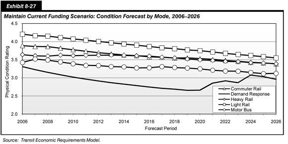
In contrast to Exhibit 8-27, which presented the projected decline in asset conditions if current reinvestment expenditures are maintained through 2026, Exhibit 8-28 presents the projected increase in the proportion of assets exceeding their useful life, by asset category, over this same time period. (Note that the proportion of assets exceeding their useful life is measured based on asset replacement values, not asset quantities). Given a level of asset reinvestment less than is required to address current reinvestment needs, the projection shows a steady increase in the proportion of assets exceeding their useful life over the 20-year projection. As in the prior exhibit, throughout this time period, systems start and end with the highest proportion of assets that exceed their useful life (using the Federal Transit Administration's useful life minimums), with the estimated proportion of over-age systems increasing from 21.6 percent in 2006 to 32.3 percent in 2026. In contrast, stations and facilities start the 20-year period with among the lowest proportion of over-age assets (roughly 7.8 and 14.3 percent, respectively) but conclude the period with roughly 19.9 and 27.1 percent or more of these assets, respectively, projected to be over-age. As with the conditions projections provided above, differences in the rate of change in the proportion of over-age assets by type reflect differences in TERM's internal prioritization of these reinvestments (based on TERM's assigned benefit-cost ratios).
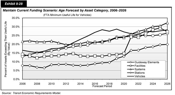
Finally, Exhibit 8-29 presents the average asset condition of all transit assets as compared to the percent of those assets that are in operation past their useful life, again assuming that rehabilitation and replacement expenditures are maintained at current levels. It is estimated that, while condition ratings decline at an average annual rate of 0.5 percent, the proportion of assets in operation in excess of their useful life continues to increase at an average rate of 3.1 percent each year from 2006 through 2026, or from 14.6 percent in 2006 to 26.9 percent by 2026.
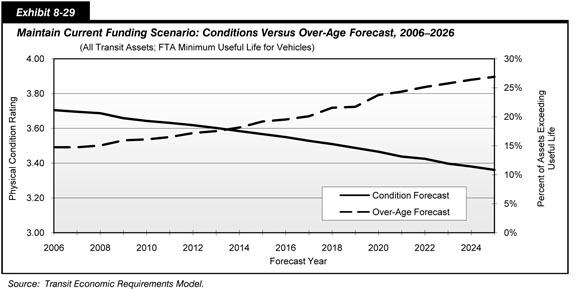
Expansion and Performance Improvement Investments
In addition to the $9.3 billion spent on transit asset rehabilitation and replacement in 2006, transit agencies spent an additional $3.5 billion on expansions to existing services to support ongoing ridership growth (roughly $2.4 billion) and on investments in new services or transit capacity to improve transit performance and attract new ridership ($1.1 billion). This section presents analysis considering how the continuation of 2006 levels of investment in expansion and performance improvement projects can be expected to impact transit service performance over the next 20 years. Specifically, the analysis compares the projected growth in transit capacity anticipated at current investment rates with projected growth in total ridership to assess the long-term impact on transit capacity utilization (i.e., average number of riders per vehicle). Once again, this analysis builds off of that already presented in Chapter 7.
Exhibit 8-30 presents the projected average vehicle occupancy by mode over the period from 2006 through 2026. These projections assume that (1) transit agencies continue to invest roughly $3.5 billion per year on expansion and capacity-related improvements and (2) that ridership will grow at rates consistent with those projected by the Nation's metropolitan planning organizations (MPOs). Despite some reductions in capacity utilization for light rail during the early years of the projection, capacity utilization for all rail modes is projected to increase over the forecast period if expansion investments maintain their current pace. Thus, recent spending levels do not appear sufficient to maintain performance in aggregate across the rail transit modes, potentially compounding existing overcrowding problems for some high demand operators. In contrast, capacity utilization for motorbus is projected to decline from 10.7 to 7.8 passengers per vehicle over this period. This projected decline for bus and the increase for rail systems results from the generally higher benefit-cost ratios generated by TERM for bus versus rail investments; hence, bus investments generally receive a higher investment priority in this budget constrained analysis. By comparison, light rail incurs a 3.0 percent increase in occupancy, while commuter rail and heavy rail average vehicle occupancy both increase by more than 25 percent between 2006 and 2026.
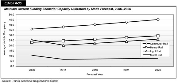
Exhibit 8-31 presents the total number of transit riders that are supported by differing levels of investment, while maintaining performance (i.e., capacity utilization) at current levels. This exhibit clearly indicates that, while continuation of the 2006 level of investment could support a significant number of new riders—more than 2 billion in additional annual boardings—this level of investment is not sufficient to support the number of new riders projected by the Nation's MPOs (almost 3.5 billion additional annual riders). Finally, investment consistent with TERM's Improve Performance scenario (as described in the next section) could support an additional 5.5 billion annual boardings over 2006 levels.
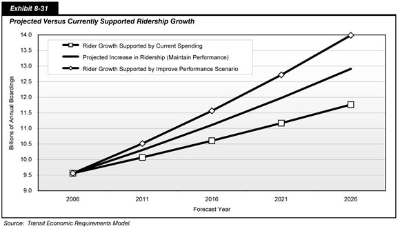
Maintain and Improve Conditions and Performance Scenarios
Since 1997, the C&P report has included a consistent set of TERM investment scenarios that assess the level of investment required to attain specific asset conditions and performance targets. The levels of investment required to attain these targets have also been combined to construct a range of investment scenarios. The specific investment targets include the following:
- Maintain Conditions scenario
Transit assets are replaced and rehabilitated over the 20-year period such that the overall average condition at the beginning of the period is identical to that at the end of the forecast period. - Maintain Performance scenario
New transit vehicles and infrastructure investments are undertaken to accommodate projected increases in transit ridership so that the vehicle utilization rate existing at the beginning of the period remains the same at the end of the period. Ridership growth estimates are obtained from MPOs. - Improve Performance scenario
Transit asset rehabilitation and replacement is accelerated to improve the average condition of all transit assets to a "Good" level at the end of the 20-year period (2026 for purposes of this report). If an average condition of good can be reached only by replacing assets that are still in operationally acceptable condition, then this scenario will target a lower condition level; this will be equal to the highest condition that can be achieved without replacing assets that are still in operationally acceptable condition. - Improve Performance scenario
The performance of the Nation's transit system is improved overall as additional investments in bus rapid transit (BRT), light rail, or heavy rail are introduced in urbanized areas with the most crowded vehicles and the slowest system speeds in order to reduce vehicle utilization rates (and crowding) and increase average transit operating speeds.
| Is the average asset condition to Maintain Conditions reached after 20 years always the same as in the base year? Does the average asset condition to Improve Conditions absolutely reach an average condition rating of 4 at the end of the 20-year period? | |
|
The Maintain Conditions scenario tries to match the average asset condition in the projected year (2026) with the average asset condition in the base year (2006). In this report, the investment needs to Maintain Conditions assume that the average condition rating will be 3.55 in 2026, compared with an average condition rating of 3.71 in 2006. To reach an average condition rating of 3.82 in 2026 would require TERM to replace some asset types at an unreasonably high condition replacement threshold (i.e., while those assets were still in an operationally acceptable condition). The Improve Conditions scenario assumes that an average asset condition rating of 3.67 will be reached in 2026. To reach a condition rating of 4.0 in 2026 would again require TERM to replace many asset types while still in an operationally acceptable condition even more (see Appendix C).
|
|
Scenario Investment Needs: Benefit-Cost Ratio of 1.0
Exhibit 8-32 presents estimates of the total annual capital investment required to attain combinations of the four investment scenarios presented above. Moreover, these needs are segmented by improvement type, including needs for rehabilitation and replacement (to maintain conditions), for asset expansion (to maintain performance), and those for performance improvement. The analysis presented in this section only includes investments with benefit-cost ratios of 1.0 or higher.
| Type of Improvement | Maintain Conditions & Performance | Improve Conditions & Maintain Performance | Maintain Conditions & Improve Performance | Improve Conditions & Performance |
|---|---|---|---|---|
| Replacement and Rehabilitation | $10.7 | $12.2 | $10.7 | $12.2 |
| Asset Expansion | $4.3 | $2.9 | $4.3 | $2.9 |
| Performance Improvements | $5.9 | $5.9 | ||
| Total | $15.1 | $15.2 | $21.0 | $21.1 |
Maintain Conditions
Replacement and rehabilitation needs to maintain asset conditions through 2026 are estimated to be $10.7 billion annually. This includes $6.0 billion for rail and $4.5 billion for nonrail modes, respectively. The $4.7 billion investment requirement for nonrail includes $0.2 billion for Special Services (Section 5310) operators.
Maintain Performance
Over the period from 2006 through 2026, the Nation's MPOs project an estimated 1.5 percent (weighted) average annual increase in boardings. The annual investment in asset expansion required to serve this projected increase while maintaining current service performance is $4.3 billion. Annual rail investment requirements are estimated at $2.9 billion, with an additional $1.5 billion for nonrail assets.
Improve Conditions
The incremental $1.5 billion for asset rehabilitation and replacement represents the additional investment required to rehabilitate and replace assets to attain an overall physical condition level of good. The average annual estimate of $1.5 billion comprises $0.6 billion for rail assets and $0.9 billion for nonrail assets.
Improve Performance
Investments to improve performance (increasing passenger speeds and reducing crowding in systems not operating at a condition of good performance threshold levels) are estimated to be $5.9 billion annually. Note that this scenario defines an upper limit above which additional investment in transit is unlikely to be economically justifiable.
Investment Estimates by Population Area Size
Exhibit 8-33 provides a detailed view of transit investments by TERM scenario, area population size, and asset type. Urban areas with populations of more than 1 million make up 88.6 percent of transit investment estimates for the Maintain Conditions and Performance scenario, reflecting the fact that, in 2006, 92 percent of the Nation's transit passenger miles were in these areas.
| Mode, Purpose, & Asset Type | (Billions of 2006 Dollars) Cost to Maintain Conditions & Performance |
(Billions of 2006 Dollars) Incremental Cost to Improve Conditions |
(Billions of 2006 Dollars) Incremental Cost to Improve Performance |
(Billions of 2006 Dollars) Cost to Improve Conditions & Performance |
|
|---|---|---|---|---|---|
| Areas More Than 1 Million in Population | |||||
| Nonrail 1 | |||||
| Replacement & Rehabilitation | (Vehicles) | $2.0 | $0.5 | $0.0 | $2.5 |
| Replacement & Rehabilitation | (Nonvehicles) 2 | $1.3 | $0.1 | $0.0 | $1.4 |
| Asset Expansion | (Vehicles) | $0.7 | $0.0 | $0.0 | $0.8 |
| Asset Expansion | (Nonvehicles) | $0.4 | $0.0 | $0.0 | $0.4 |
| Improve Performance | (Vehicles) | $0.0 | $0.0 | $0.4 | $0.4 |
| Improve Performance | (Nonvehicles) 2 | $0.0 | $0.0 | $0.2 | $0.2 |
| Special Service 3 | (Vehicles) | $0.0 | $0.0 | $0.0 | $0.0 |
| Subtotal Nonrail 4 | $4.5 | $0.6 | $0.6 | $5.7 | |
| Rail | |||||
| Replacement & Rehabilitation | (Vehicles) | $0.8 | $0.4 | $0.0 | $1.2 |
| Replacement & Rehabilitation | (Nonvehicles) 2 | $5.2 | $0.2 | $0.0 | $5.4 |
| Asset Expansion | (Vehicles) | $0.7 | -$0.3 | $0.0 | $0.4 |
| Asset Expansion | (Nonvehicles) 2 | $2.1 | -$1.1 | $0.0 | $1.1 |
| Improve Performance | (Vehicles) | $0.0 | $0.0 | $0.6 | $0.6 |
| Improve Performance | (Nonvehicles) 2 | $0.0 | $0.0 | $4.0 | $4.0 |
| Subtotal Rail 4 | $8.8 | -$0.8 | $4.6 | $12.7 | |
| Total Areas More Than 1 Million4 | $13.3 | -$0.2 | $5.2 | $18.4 | |
| Areas Less Than 1 Million in Population | |||||
| Nonrail 1 | |||||
| Replacement & Rehabilitation | (Vehicles) | $0.7 | $0.2 | $0.0 | $0.9 |
| Replacement & Rehabilitation | (Nonvehicles) 2 | $0.5 | $0.1 | $0.0 | $0.5 |
| Fleet Expansion | (Vehicles) | $0.2 | $0.0 | $0.0 | $0.2 |
| Fleet Expansion | (Nonvehicles) 2 | $0.1 | $0.0 | $0.0 | $0.1 |
| Improve Performance | (Vehicles) | $0.0 | $0.0 | $0.2 | $0.2 |
| Improve Performance | (Nonvehicles) 2 | $0.0 | $0.0 | $0.5 | $0.5 |
| Special Service 3 | (Vehicles) | $0.2 | $0.1 | $0.0 | $0.3 |
| Subtotal Nonrail 4 | $1.7 | $0.3 | $0.7 | $2.7 | |
| Rail | |||||
| Replacement & Rehabilitation | (Vehicles) | $0.0 | $0.0 | $0.0 | $0.0 |
| Replacement & Rehabilitation | (Nonvehicles) 2 | $0.0 | $0.0 | $0.0 | $0.0 |
| Fleet Expansion | (Vehicles) | $0.0 | $0.0 | $0.0 | $0.0 |
| Fleet Expansion | (Nonvehicles) 2 | $0.0 | $0.0 | $0.0 | $0.0 |
| Improve Performance | (Vehicles) | $0.0 | $0.0 | $0.0 | $0.0 |
| Improve Performance | (Nonvehicles) 2 | $0.0 | $0.0 | $0.0 | $0.0 |
| Subtotal Rail 4 | $0.0 | $0.0 | $0.0 | $0.0 | |
| Total Areas Less Than 1 Million 4 | $1.7 | $0.3 | $0.7 | $2.7 | |
| Total 4 | $15.1 | $0.1 | $5.9 | $21.1 | |
The Maintain Conditions and Performance scenario estimates an average annual investment of $13.3 billion to maintain the conditions and performance of transit assets in large urban areas; the Improve Conditions and Performance scenario estimates an average annual investment of $18.4 billion annually to improve the conditions and performance of transit assets in large urban areas. The investment in less-populated areas (i.e., those urban areas with populations of less than 1 million) is estimated to be considerably lower than the investment in more populous areas because the former have fewer transit assets. The Maintain Conditions and Performance scenario estimates an average investment of $1.7 billion annually in the transit infrastructure in these less-populated areas, and the Improve Conditions and Performance scenario estimates an average investment of $2.7 billion annually in transit infrastructure in these less-populated areas.
Nonrail Needs in Areas With Populations of More Than 1 Million
The nonrail infrastructure component (buses, vans, and ferryboats) of the Maintain Conditions and Performance scenario in urban areas with populations over 1 million is considerably smaller than the rail component. The Maintain Conditions and Performance scenario estimates that 33.8 percent of the investment in larger urban areas, or about $4.5 billion annually, is for nonrail infrastructure. Of this $4.5 billion, 74.3 percent, or $3.3 billion annually, is estimated for the rehabilitation and replacement of assets, and 25.0 percent, or $1.1 billion, is estimated for the purchase of new assets to maintain performance. It is estimated that 60.4 percent of rehabilitation and replacement expenditures and 66.3 percent of asset expansion expenditures would be for vehicles. The incremental costs to improve nonrail conditions are estimated to be $580 million annually, of which 78.4 percent ($455 million) would be for vehicle rehabilitation and replacement. The incremental costs to improve performance are estimated to be $619 million annually, of which 65.0 percent ($402 million) would be spent on new vehicles (principally buses) and 35.0 percent ($217 million) on new nonvehicle assets. Expenditures on nonvehicle assets include investments for the purchase or construction of dedicated highway lanes for BRT. The Improve Conditions and Performance scenario estimates that, in total, $5.7 billion is needed for investment in these more heavily populated areas.
Rail Needs in Areas With Populations of More Than 1 Million
The Maintain Conditions and Performance scenario estimates that 66.2 percent of the total transit investment in large urban areas, or $8.8 billion annually, is for rail infrastructure. Of this $8.8 billion, 67.7 percent, or $6.0 billion annually, is for the rehabilitation and replacement of rail assets to maintain conditions, and 32.3 percent, or $2.8 billion, is for the purchase of new assets to expand rail systems as ridership increases. The Improve Performance scenario estimates an additional amount of $4.6 billion annually for rail assets, including the cost of purchasing rights-of-way. Eighty-seven percent of the $4.6 billion performance investments for rail, or $4.0 billion, is for nonvehicle rail infrastructure. The split between vehicle and nonvehicle investment for performance improvement is within the range of what is typical for new heavy and light rail infrastructure development projects. A total of $12.7 billion annually is estimated by the Improve Conditions and Performance scenario for rail in these more heavily populated, urbanized areas.
Nonrail Needs in Areas With Populations of Less Than 1 Million
Based on the Maintain Conditions and Performance scenario, 99.1 percent of transit investment in areas with populations under 1 million is estimated for nonrail transit. The Maintain Conditions and Performance scenario estimates an investment of $1.7 billion annually in the nonrail transit infrastructure in these less-populated areas; and the Improve Conditions and Performance scenario estimates it to be $2.7 billion annually. The incremental investment estimated to improve conditions in these areas is $0.3 billion annually, and the incremental investment to improve performance is $0.7 billion. Of the $0.7 billion incremental annual investment to improve performance, 29.8 percent, or $0.2 billion, would be needed to acquire new vehicles, and 70.2 percent, or $0.5 billion, would be needed for investment in the new nonvehicle infrastructure. This edition of the C&P report assumes that investment required to improve speed will be in the form of BRT rather than light rail, except in systems where rail already exists. This assumption was also made for the 2006 Report. The 2002 C&P Report and earlier editions assumed that all investment to increase speeds in these less populous areas would be in light rail.
Rail Needs in Areas With Populations of Less Than 1 Million
The investment scenarios find that rail needs in areas with populations of less than 1 million are minimal. Six light rail systems currently operate in these less-populated areas. The Maintain Conditions and Performance scenario estimates investment in rail for these areas to be $15.3 million annually. Eighty-eight percent of the $15.3 million, or $13.1 million annually, is for investment in nonvehicle rail infrastructure. For the Improve Conditions and Performance scenario, an additional $2.7 million would be required to support vehicle rehabilitation and replacement.
Investment Estimates by Asset Type
Exhibit 8-34 provides disaggregated annual investment by scenario for rail and nonrail transportation modes by asset type for asset replacement and rehabilitation, asset expansion, and performance improvement.
| Maintain Conditions and Performance | ||||
|---|---|---|---|---|
| Asset Type | Rehabilitation and Replacement | Asset Expansion | Improve Performance | Total |
| Rail | ||||
| Guideway Elements | $1.8 | $0.7 | $0.0 | $2.5 |
| Facilities | $0.5 | $0.1 | $0.0 | $0.6 |
| Systems | $1.9 | $0.2 | $0.0 | $2.1 |
| Stations | $0.9 | $0.4 | $0.0 | $1.3 |
| Vehicles | $0.8 | $0.7 | $0.0 | $1.6 |
| Other Project Costs | $0.7 | $0.0 | $0.7 | |
| Subtotal Rail1 | $6.0 | $2.9 | $0.0 | $8.9 |
| Nonrail | ||||
| Guideway Elements | $0.3 | $0.1 | $0.0 | $0.3 |
| Facilities | $1.4 | $0.3 | $0.0 | $1.8 |
| Systems | $0.1 | $0.0 | $0.0 | $0.1 |
| Stations | $0.0 | $0.0 | $0.0 | $0.1 |
| Vehicles | $2.9 | $1.0 | $0.0 | $3.9 |
| Other Project Costs | $0.0 | $0.0 | $0.0 | |
| Subtotal Nonrail1 | $4.7 | $1.5 | $0.0 | $6.2 |
| Total Maintain Conditions1 | $10.7 | $4.3 | $0.0 | $15.1 |
| Improve Conditions and Performance | ||||
| Rail | ||||
| Guideway Elements | $1.9 | $0.4 | $1.2 | $3.5 |
| Facilities | $0.5 | $0.0 | $0.1 | $0.7 |
| Systems | $2.1 | $0.1 | $0.3 | $2.5 |
| Stations | $0.9 | $0.2 | $0.8 | $1.9 |
| Vehicles | $1.2 | $0.4 | $0.6 | $2.2 |
| Other Project Costs | $0.3 | $1.5 | $1.9 | |
| Subtotal Rail1 | $6.6 | $1.5 | $4.6 | $12.7 |
| Nonrail | ||||
| Guideway Elements | $0.3 | $0.1 | $0.2 | $0.5 |
| Facilities | $1.6 | $0.3 | $0.3 | $2.2 |
| Systems | $0.1 | $0.0 | $0.0 | $0.1 |
| Stations | $0.0 | $0.0 | $0.1 | $0.1 |
| Vehicles | $3.7 | $1.0 | $0.6 | $5.3 |
| Other Project Costs | $0.0 | $0.1 | $0.1 | |
| Subtotal Nonrail1 | $5.6 | $1.5 | $1.3 | $8.4 |
| Total Improve Conditions1 | $12.2 | $2.9 | $5.9 | $21.1 |
Assets are disaggregated into five categories—guideway elements, facilities, systems, stations, and vehicles. The estimates of annual funding for services to support investment in new transit capacity are provided under "Other Project Costs." These costs include expenditures for project design, project management and oversight, right-of-way acquisition, and site preparation.
Rail Infrastructure
Fifty-nine percent of the total amount estimated by the Maintain Conditions and Performance scenario ($8.9 billion dollars annually) and 60.1 percent of the total amount estimated by the Improve Conditions and Performance scenario ($12.7 billion annually) are for rail infrastructure. Guideway elements and systems are estimated to have the largest amounts of the total capital investment of all rail assets between 2007 and 2026, followed by vehicles, stations, and facilities in descending order of investment.
Guideways are estimated to account for 44.3 percent of the total value of the Nation's rail infrastructure. [See the "Value of U.S. Transit Assets" section in Chapter 3.] Twenty-eight percent of the total amount of the investment in the Nation's transit rail assets estimated by the Maintain Conditions and Performance and Improve Conditions and Performance scenarios is for guideway elements, comprising elevated structures, systems structures, and track—assets with long, useful lives relative to most other transit assets. The Maintain Conditions and Performance scenario estimates annual rail guideway investment to be $2.5 billion, and the Improve Conditions and Performance scenario estimates annual guideway investment to be $3.5 billion. For guideway elements, the Maintain Conditions scenario estimates annual rehabilitation and replacement to be $1.8 billion, the Maintain Performance scenario estimates annual asset expansions to cost $0.7 billion, and the Improve Performance scenario estimates no investments annually. The amount estimated by the Improve Conditions scenario, for guideway elements, annual rehabilitation and replacement to be $1.9 billion, the Improve Conditions scenario estimates annual asset expansions to cost $0.4 billion, and the Improve Performance scenario estimates investments of $1.2 billion annually.
Vehicles are estimated to account for 11.6 percent of the total value of the Nation's rail infrastructure. Eighteen percent of the amount estimated to maintain rail asset conditions and performance, or $1.6 billion annually, and 17.5 percent of the amount estimated to improve rail asset conditions and performance, or $2.2 billion annually, are for vehicles. Annual vehicle rehabilitation and replacement costs are estimated to be $0.8 billion to maintain conditions and $1.2 billion to improve conditions. Annual asset expansion costs are estimated to be $0.7 billion to maintain performance and $0.4 billion to improve performance.
Rail systems, comprising train control, traction power, and communications, are estimated to account for 22.0 percent of the total value of the Nation's rail asset base. Twenty-four percent of the amount estimated to maintain the conditions and performance of rail assets, or $2.1 billion annually, and 20.0 percent of the amount estimated to improve the conditions and performance of rail assets, or $2.5 billion annually, are for rail systems. Annual rehabilitation and replacement costs are estimated to be $1.9 billion to maintain conditions and $2.1 billion to improve conditions. Annual asset expansion costs are estimated to be $0.2 billion to maintain rail power system performance and an additional $0.1 billion to improve performance.
Stations are estimated to account for 16.0 percent of the total value of the Nation's rail infrastructure. Fifteen percent of the amount estimated to maintain the conditions and performance of rail assets, or $1.3 billion annually, and 15.1 percent of the annual amount estimated to improve the conditions and performance of rail assets, or $1.9 billion annually, are estimated to be for stations. The amount estimated for rehabilitation and replacement both to maintain rail station conditions and to improve rail station conditions is estimated to be $0.9 billion. The annual amount of station expansion to maintain performance is estimated to be $0.4 billion. To improve performance, the annual amount of station expansion investment required is estimated to be $0.2 billion.
Facilities for rail vehicles (maintenance facilities and yards) are estimated to account for 6.1 percent of the total value of the Nation's rail transit asset base. Seven percent of the amount to maintain conditions, $0.6 billion annually, and 5.3 percent of the amount to improve conditions and performance, $0.7 billion annually, are estimated to be for facilities. Annual rehabilitation and replacement costs are estimated to be $0.5 billion both to maintain and to improve conditions. Asset expansion costs are estimated to be $0.1 billion annually for maintain performance and $42 million annually to improve performance.
Nonrail Assets
Forty-one percent of the total amount to maintain conditions and performance, or $6.2 billion dollars annually, and 39.9 percent of the total amount estimated to improve conditions and performance, or $8.4 billion annually, are for nonrail infrastructure. Vehicles are estimated to require the largest amount of the total capital investment in nonrail assets between 2007 and 2026, followed in descending order of estimated investment by facilities, guideway elements (dedicated lanes for buses), stations, and systems.
Vehicles are estimated to account for 31.7 percent of the total value of the Nation's nonrail assets, excluding vehicles in rural areas. (Note that asset value is estimated by TERM, which does not include rural operators.) However, they account for substantially more of estimated nonrail investment because they depreciate much more quickly than nonvehicle assets. The investment in nonrail vehicles estimated by the Maintain Conditions and Performance scenario is $3.9 billion annually, and the investment in nonrail estimated by the Improve Conditions and Performance scenario is $5.3 billion annually. Sixty-two percent of estimated nonrail rehabilitation and replacement expenditures by the Maintain Performance scenario is for vehicles, while 65.1 percent of estimated nonrail rehabilitation and replacement expenditures by the Improve Performance scenario is for vehicles. Vehicles are also estimated to account for the largest proportion, about 67.7 percent, of nonrail asset expansion investments by the Maintain Performance scenario and 68.3 percent of the amount estimated by the Improve Performance scenario.
Facilities are estimated to account for 52.3 percent of the total value of the Nation's nonrail assets, excluding facilities in rural areas. Although facilities account for more than half of the nonrail assets, it is estimated that they will account for over 28.6 percent of future nonrail investment in the Maintain Conditions and Performance scenario because external structures and many of the facility components depreciate slowly. The Maintain Conditions and Performance scenario estimates investment in facilities to be $1.8 billion, and the Improve Conditions and Performance scenario estimates investment in facilities to be $2.2 billion.
Guideway elements account for 10.3 percent of the Nation's nonrail assets, stations account for 3 percent, and power systems account for 1.8 percent. The Maintain Conditions and Performance scenario estimates investment of $0.3 billion annually for nonrail guideway, and the Improve Conditions and Performance scenario estimates investment of $0.5 billion for nonrail guideway. These amounts decreased principally due to revisions in the benefit-cost analysis and updated NTD data. The Maintain Conditions and Performance scenario estimates investment of $0.1 billion annually for nonrail stations, and the Improve Conditions and Performance scenario estimates investment of $0.1 billion for nonrail stations. The Maintain Conditions and Performance scenario estimates investment of $0.1 billion annually in nonrail systems; and the Improve Conditions and Performance scenario estimates investment of $0.1 billion in nonrail systems.
Scenario Investment Needs: Benefit-Cost Ratio of 1.2
The analysis presented in the previous section included all investments with a benefit-cost ratio of 1.0 or higher. In contrast, this section reproduces each of the scenarios considered above, but this time only including those investments with a benefit-cost ratio of 1.2 or higher. By assessing the sensitivity of the estimated investment needs to changes in the underlying benefit-cost ratio, this analysis provides an indication of the proportion of investments expected to provide high returns versus those expected to provide more marginal investment returns. To facilitate this comparison, Exhibit 8-35 below presents a summary of the annual transit investment requirements by TERM investment scenario and type of improvement where the benefit-cost ratio is greater than or equal to 1.0 and 1.2, and the variance between the two scenarios.
| TERM Investment Scenario Type of Improvement |
Maintain Conditions & Performance BCR 1.0 |
Maintain Conditions & Performance BCR 1.2 |
Maintain Conditions & Performance Difference |
Improve Conditions & Performance BCR 1.0 |
Improve Conditions & Performance BCR 1.2 |
Improve Conditions & Performance Difference |
|---|---|---|---|---|---|---|
| Replacement and Rehabilitation Rail |
$6.0 | $0.7 | $6.6 | $0.4 | ||
| Replacement and Rehabilitation Nonrail |
$4.7 | $3.2 | $5.6 | $3.7 | ||
| Replacement and Rehabilitation Total |
$10.7 | $3.9 | $12.2 | $4.1 | ||
| Asset Expansion Rail |
$2.9 | $0.6 | $1.5 | $0.4 | ||
| Asset Expansion Nonrail |
$1.5 | $1.1 | $1.5 | $1.1 | ||
| Asset Expansion Total |
$4.3 | $1.7 | $2.9 | $1.5 | ||
| Performance Improvements Rail |
$0.0 | $0.0 | $4.6 | $3.2 | ||
| Performance Improvements Nonrail |
$0.0 | $0.0 | $1.3 | $1.3 | ||
| Performance Improvements Total |
$0.0 | $0.0 | $5.9 | $4.5 | ||
| Total Rail |
$8.9 | $1.3 | $12.7 | $4.0 | ||
| Total Nonrail |
$6.2 | $4.3 | $8.4 | $6.1 | ||
| Total Total |
$15.1 | $5.6 | $21.1 | $10.2 |
Based on the analysis below, TERM estimates show some sensitivity to changes in the benefit-cost ratio. Moreover, this sensitivity is apparent for all investment types, including those to maintain or improve conditions and those to maintain or improve performance.
Maintain Conditions
The annual amount estimated by TERM under the Maintain Conditions and Performance scenario baseline at a benefit-cost ratio of 1.0 for the Nation's rail and nonrail transit infrastructure is $10.7 billion annually. By increasing the benefit-cost ratio from 1.0 to 1.2, a decrease of 63.4 percent in investment requirements is realized on the annual cost to maintain conditions and performance, yielding an average annual investment requirement of $3.9 billion. For the baseline scenario with a benefit-cost ratio of 1.2, the average annual amount estimated by TERM for replacement and rehabilitation of the Nation's transit assets between 2007 and 2026 is $0.7 billion for rail and $3.2 billion for nonrail, compared with rail investment requirements of $6.0 billion and nonrail investment requirements of $4.7 billion annually with a benefit-cost ratio of 1.0.
| How does TERM screen proposed investments? | |
|
All investments identified by TERM's capital investment needs estimates must successfully pass the model's benefit-cost test. If an investment fails that test, it is rejected and the cost of that investment is not added to the model's tally of national transit investment needs. If the investment passes the benefit-cost test, the investment needs tally is updated to include that investment's costs. All of TERM's benefit-cost tests evaluate the benefits and costs of each proposed investment over a 20-year time period. For most analyses, the ratio of benefits to costs must equal or exceed a value of 1.0 to pass the benefit-cost test. This subsection only considers investments with benefit-cost ratios greater than or equal to 1.2.
|
|
Maintain Performance
To accommodate asset expansion, an additional $0.6 billion annually is required for rail assets and an additional $1.1 billion is required for nonrail assets under the 1.2 benefit-cost ratio scenario, compared with $2.9 billion for rail assets and $1.5 billion for nonrail assets under the 1.0 scenario.
Improve Conditions
The average annual amount estimated by TERM to improve conditions decreases from $12.2 billion in the 1.0 benefit-cost ratio scenario to $4.1 billion in the 1.2 benefit-cost ratio scenario, with $0.4 billion required for rail and $3.7 billion for nonrail. It is interesting to note that rail investment requirements decreased more significantly than nonrail requirements due to a higher benefit-cost ratio on average for bus than rail. Most bus benefit-cost ratios are significantly further from 1.2, while rail aligns closer to 1.0.
Improve Performance
The investment to improve service performance for rail assets over the period 2007 to 2026 declined from the $4.6 billion under the benefit-cost ratio of 1.0 scenario to $3.2 billion annually under the benefit-cost ratio of 1.2. For nonrail assets, annual investments required to improve performance are the same for both benefit-cost ratio scenarios with an estimate of $1.3 billion per year.
Maintain and Improve Conditions and Performance Scenarios Assuming Highway Congestion Pricing
The highway congestion pricing scenarios examined in this and other chapters of this edition of the C&P report assume that a portion of the reduction in vehicle miles traveled (VMT) resulting from the imposition of highway congestion pricing is diverted to transit (see "Projected VMT in 2026" section in Chapter 7). This section considers the level of expansion investment required to support this increase in transit ridership while maintaining current transit performance (measured as vehicle capacity utilization) at today's levels. To do so, the analysis assumes that between 25 percent and 50 percent of diverted automobile users shift to transit as their preferred modal choice. The remaining diverted highway users are assumed to telecommute, defer their trip, or identify other alternative modes of transportation.
| How did TERM analyze the effects of congestion pricing on transit? | |
|
Chapter 7 analyzed the potential effects of congestion pricing as an alternative funding mechanism for highway capital investments. The results of the analysis demonstrate that as highway user costs rise, vehicle miles traveled fall as travelers move to less expensive forms of transportation.
In analyzing the effects of congestion pricing on transit, TERM treated the assumed diversion of highway travelers to transit as a one-time increase in the number of transit passenger miles. The model then estimated the level of expansion investment in rail and bus vehicles, stations, guideways, and other asset types as required to support the increase in travel demand while maintaining existing vehicle occupancy rates.
|
|
This analysis leverages both the transit and highways investment scenarios. As referenced earlier in this chapter, the Sustain Current Spending (SCS) scenario for highways assumes that highway capital spending is maintained in constant dollar terms at base year 2006 levels over the 20-year period from 2007 through 2026. The Maximum Economic Investment (MEI) scenario for highways assumes that combined public and private highway capital investment gradually increases in constant dollar terms over 20 years up to the point at which all potentially cost-beneficial investments (i.e., those with a benefit-cost ratio of 1.0 or higher) are funded by 2026. Each highway scenario is projected to result in different levels of congestion, average highway user costs, and future highway VMT. As future highway congestion is projected to be worse under the SCS scenario than the MEI scenario, the average highway congestion charges imposed under the SCS scenario are higher, resulting in more potential diversion of highway VMT to transit. This results in an increase in passenger miles traveled (PMT) ranging from 2.3 percent and 4.3 percent depending on the highways investment scenario, as presented in Exhibit 8-36.
| 25% Diversion | 50% Diversion | |
|---|---|---|
| Maximum Economic Investment | 2.3% | 2.9% |
| Sustain Current Spending | 3.1% | 4.3% |
The analysis below presents the total level of transit expansion investment required to support each of these projected increases in transit ridership. As with the scenario analysis discussed above, this analysis is presented first for all those projects with a passing benefit-cost ratio of 1.0 or higher. The analysis is then repeated for projects with a benefit-cost ratio of 1.2 or higher. Once again, this approach suggests significant variation in the relative investment returns of these investment scenarios.
Benefit-Cost Ratio of 1.0
Exhibit 8-37 presents the annual level of transit investment required to support VMT diverted from highways to transit over the time period from 2007 through 2026 for projects with a benefit-cost ratio of 1.0 or higher. In comparison with the investment scenarios discussed in the prior section of this report (i.e., the scenarios for maintaining or improving conditions and performance), a significant amount of the increased need is reflected in the "Asset Expansion" category. There is also a modest increase in the level of investment needed for rehabilitation and replacement required to maintain the expanded asset base.
| Highway Investment Scenario Percent of Reduced Highway VMT Diverted to Transit Type of Improvement |
Sustain Current Spending 25% |
Sustain Current Spending 50% |
Maximum Economic Investment 25% |
Maximum Economic Investment 50% |
|---|---|---|---|---|
| Replacement and Rehabilitation (Maintain Conditions) Rail |
$6.1 | $6.8 | $6.1 | $6.8 |
| Replacement and Rehabilitation (Maintain Conditions) Nonrail |
$4.8 | $5.0 | $4.7 | $5.0 |
| Replacement and Rehabilitation (Maintain Conditions) Total |
$10.9 | $11.8 | $10.8 | $11.8 |
| Replacement and Rehabilitation (Improve Conditions) Rail |
$6.2 | $7.0 | $6.2 | $7.0 |
| Replacement and Rehabilitation (Improve Conditions) Nonrail |
$5.1 | $5.3 | $5.0 | $5.3 |
| Replacement and Rehabilitation (Improve Conditions) Total |
$11.3 | $12.3 | $11.3 | $12.3 |
| Asset Expansion (Maintain Performance) Rail |
$4.7 | $5.3 | $4.7 | $6.2 |
| Asset Expansion (Maintain Performance) Nonrail |
$3.1 | $5.0 | $2.7 | $4.3 |
| Asset Expansion (Maintain Performance) Total |
$7.8 | $10.3 | $7.4 | $10.6 |
| Performance Improvements Rail |
$4.6 | $4.6 | $4.6 | $4.6 |
| Performance Improvements Nonrail |
$1.3 | $1.3 | $1.3 | $1.3 |
| Performance Improvements Total |
$5.9 | $5.9 | $5.9 | $5.9 |
| Total Rail |
$15.5 | $16.8 | $15.4 | $17.7 |
| Total Nonrail |
$9.1 | $11.3 | $8.7 | $10.6 |
| Total Total |
$24.6 | $28.0 | $24.1 | $28.3 |
| TERM Scenario Totals Maintain Conditions and Performance |
$18.7 | $22.1 | $18.2 | $22.4 |
| TERM Scenario Totals Improve Conditions and Performance |
$25.0 | $28.5 | $24.6 | $28.8 |
Maintain Conditions
The average annual amount estimated by TERM for replacement and rehabilitation of the Nation's transit assets between 2007 and 2026, assuming that 25 percent of highway VMT is diverted to transit, is $6.1 billion for rail and $4.8 billion for nonrail. The diversion of highway VMT to transit yields an increase of only 1.9 percent in the Maintain Conditions scenario on annual transit investment requirements. However, if 50 percent of reduced VMT resulting from highway congestion pricing was diverted to transit, the Maintain Conditions scenario investment requirements would increase 10.3 percent on an annual basis, to $11.8 billion. Estimates for the highway MEI scenario under the Maintain Conditions scenario are relatively consistent with the estimated annual investment requirements for both the 25- and 50-percent scenarios. Nonrail investment requirements show a slight decline in the 25-percent scenario, from $4.8 billion to $4.7 billion.
Maintain Performance
Given the projected increase in demand for transit services from 2007 through 2026 in terms of PMT, coupled with the transition of 25 percent of reduced highway VMT to transit, TERM estimates that $7.8 billion will be required on an annual basis for investments to maintain performance at current service levels. This represents an increase from $2.9 billion for rail in the baseline to $4.7 billion under the congestion pricing scenario, and from $1.5 billion to $3.1 billion for nonrail assets to accommodate the asset expansion. To support 50 percent of highway VMT diverting to transit, an estimated $10.3 billion would be required on an annual basis in the highway SCS scenario and $10.6 billion under the MEI scenario.
The annual amount estimated by TERM under the Maintain Conditions and Performance scenario within the highway SCS investment scenario for the Nation's rail and nonrail transit infrastructure is $18.7 billion for a 25-percent diversion of reduced highway VMT to transit and $22.1 billion for a 50-percent diversion. Similarly, the annual amount estimated by TERM to maintain current conditions and performance under the highway MEI investment scenario is $18.2 billion for a 25-percent diversion of reduced highway VMT to transit and $22.4 billion for a 50-percent diversion.
Improve Conditions
The average annual amount estimated by TERM to improve conditions of the Nation's transit assets between 2007 and 2026, assuming that 25 percent of highway VMT is diverted to transit, is $6.2 billion for rail and $5.1 billion for nonrail under the Highway Congestion Pricing SCS scenario. Under the MEI scenario, nonrail requirements decline to $5.0 billion. However, if 50 percent of reduced VMT resulting from highway congestion pricing was diverted to transit, the Improve Conditions scenario investment requirements would increase 8.8 percent on an annual basis, to $7.0 billion for rail, and $5.3 billion for nonrail. Estimates for the highway MEI and SCS scenarios under the Improve Conditions scenario are relatively consistent with the estimated annual investment requirements for both the 25- and 50-percent scenarios.
Improve Performance
The average annual amount estimated by TERM to improve performance assuming highway congestion pricing is consistent with the baseline requirements, at $4.6 billion for rail and $1.3 billion for nonrail, to support the additional riders resulting from the VMT shift. Further, the investment required to improve performance is consistent between the two VMT scenarios at a total of $5.9 billion annually. Estimates for the Performance Improvement scenario are consistent per the MEI for both the 25-percent and 50-percent scenarios. The congestion pricing scenarios only have a direct impact on Maintain Performance scenario investments, which are modeled by increasing PMT growth rates. The Maintain Conditions scenario may also be impacted because the benefit-cost tests are tied together for the Maintain Performance and Maintain and Improve Condition investments (on an agency-mode basis). In contrast, there is no link between the Maintain Performance and Improve Performance modules for this analysis.
Benefit-Cost Ratio of 1.2
Exhibit 8-38 presents the annual level of transit investment required to support VMT diverted from highways to transit over the 2007 to 2026 time period for projects with a benefit-cost ratio of 1.2 or higher.
| Highway Investment Scenario Percent of Reduced Highway VMT Diverted to Transit Type of Improvement |
Sustain Current Spending 25% |
Sustain Current Spending 50% |
Maximum Economic Investment 25% |
Maximum Economic Investment 50% |
|---|---|---|---|---|
| Replacement and Rehabilitation (Maintain Conditions) Rail |
$1.4 | $5.1 | $1.4 | $4.8 |
| Replacement and Rehabilitation (Maintain Conditions) Nonrail |
$3.5 | $3.5 | $3.4 | $3.5 |
| Replacement and Rehabilitation (Maintain Conditions) Total |
$4.9 | $8.6 | $4.8 | $8.3 |
| Replacement and Rehabilitation (Improve Conditions) Rail |
$0.9 | $5.3 | $1.6 | $5.0 |
| Replacement and Rehabilitation (Improve Conditions) Nonrail |
$3.0 | $3.9 | $3.7 | $3.8 |
| Replacement and Rehabilitation (Improve Conditions) Total |
$4.0 | $9.2 | $5.3 | $8.8 |
| Asset Expansion (Maintain Performance) Rail |
$0.8 | $3.4 | $0.8 | $3.4 |
| Asset Expansion (Maintain Performance) Nonrail |
$2.7 | $4.3 | $2.4 | $3.8 |
| Asset Expansion (Maintain Performance) Total |
$3.5 | $7.8 | $3.2 | $7.2 |
| Performance Improvements Rail |
$3.2 | $3.2 | $3.2 | $3.2 |
| Performance Improvements Nonrail |
$1.3 | $1.3 | $1.3 | $1.3 |
| Performance Improvements Total |
$4.5 | $4.5 | $4.5 | $4.5 |
| Total Rail |
$5.5 | $11.8 | $5.4 | $11.5 |
| Total Nonrail |
$7.4 | $9.0 | $7.0 | $8.6 |
| Total Total |
$12.8 | $20.9 | $12.5 | $20.1 |
| TERM Scenario Totals Maintain Conditions and Performance |
$8.3 | $16.4 | $8.0 | $15.6 |
| TERM Scenario Totals Improve Conditions and Performance |
$11.9 | $21.4 | $13.0 | $20.5 |
Maintain Conditions
With a benefit-cost ratio of 1.2, the average annual amount estimated by TERM for replacement and rehabilitation of the Nation's transit assets between 2007 and 2026, assuming that 25 percent of reduced highway VMT were diverted to transit under the SCS scenario, increases from $3.9 billion in the baseline analysis to $4.9 billion for rail and nonrail assets. If 50 percent of VMT were diverted to transit, the Maintain Conditions scenario investment requirements increase to an estimated $8.6 billion again, compared with $3.9 billion in the baseline Maintain Conditions and Performance scenario with a benefit-cost ratio of 1.2.
For the MEI scenarios, average annual investment requirement for the Maintain Conditions scenario increases in both the 25- and 50-percent scenarios in comparison to the baseline analysis, with a benefit-cost ratio of 1.2, from $3.9 billion to $4.8 billion at the 25-percent scenario and $8.3 billion for the 50-percent scenario.
Maintain Performance
Given the projected increase in demand for transit services from 2007 through 2026 in PMT, coupled with the transition of 25 percent of reduced highway VMT to transit, TERM estimates that $3.5 billion will be required on an annual basis for investments to maintain performance at current service levels for both rail and nonrail assets in the SCS scenario; under the MEI scenario, this decreases to $3.2 billion. This is in comparison to $1.7 billion in annual investment requirements in the baseline with a benefit-cost ratio of 1.2. To support 50 percent of reduced highway VMT diverting to transit, an estimated $7.8 billion would be required on an annual basis under SCS, with $3.4 billion required for rail and $4.3 billion for nonrail assets. Under the constraints of the MEI scenario, the annual investment requirement declines to $7.2 billion, resulting from a decline in nonrail requirements.
The annual amount estimated by TERM under the Maintain Conditions and Performance scenario for the Nation's rail and nonrail transit infrastructure is $8.3 billion for a 25-percent diversion of highway VMT to transit and $16.4 billion for a 50-percent diversion under the highway SCS scenario. The baseline analysis with a benefit-cost ratio of 1.2 shows $5.6 billion in annual investment requirements.
Under the highway MEI scenario, the annual amount estimated by TERM under the Maintain Conditions and Performance scenario for the Nation's rail and nonrail transit infrastructure is $8.0 billion for a 25- percent diversion of highway VMT to transit and $15.6 billion for a 50-percent diversion. Again, the baseline analysis with a benefit-cost ratio of 1.2 shows $5.6 billion in annual investment requirements.
Improve Conditions
With a benefit-cost ratio of 1.2, the average annual amount estimated by TERM to improve conditions of the Nation's transit assets between 2007 and 2026, assuming that 25 percent of reduced highway VMT were diverted to transit under the SCS scenario, is estimated at $0.9 billion for rail and $3.0 billion for nonrail assets. If 50 percent of VMT were diverted to transit, the Improve Conditions scenario investment requirements increase to an estimated $5.3 billion for rail, and $3.9 billion for nonrail assets. For the MEI scenario, average annual investment requirement for the Improve Conditions scenario is estimated at $5.3 billion at the 25-percent scenario and $8.8 billion for the 50-percent scenario.
Improve Performance
The average annual amount estimated by TERM to improve performance is consistent with the baseline requirements with a benefit-cost ratio of 1.2 at $3.2 billion for rail and $1.3 billion for nonrail to support the additional riders resulting from the VMT shift. Further, the investment required to improve performance is consistent between the two VMT scenarios with a benefit-cost ratio of 1.2, at a total of $4.5 billion annually. Estimates for the Performance Improvement scenario are also consistent between the SCS and MEI scenarios for both the 25-percent and 50-percent scenarios.
The annual amount estimated by TERM under the Improve Conditions and Performance scenario for the Nation's rail and nonrail transit infrastructure is $11.9 billion for a 25-percent diversion of highway VMT to transit and $21.4 billion for a 50-percent diversion under the highway SCS scenario. This is in comparison to the baseline analysis with a benefit-cost ratio of 1.2 that results in $10.2 billion in annual investment requirements for the Improve Conditions and Performance scenario.
Under the highway MEI scenario, the annual amount estimated by TERM under the Improve Conditions and Performance scenario for the Nation's rail and nonrail transit infrastructure is $13.0 billion for a 25- percent diversion of highway VMT to transit and $20.5 billion for a 50-percent diversion. Again, the baseline analysis with a benefit-cost ratio of 1.2 shows $10.2 billion in annual investment requirements.
Alternative Benefit-Cost Ratio Thresholds
The transit analysis presented in this chapter has considered the impact of increasing the benefit-cost ratio from 1.0 to 1.2 on TERM's total needs assessments. In general, this increase resulted in a significant decline in estimated needs, suggesting that there is a broad range of investment returns for those investments considered by the model. Exhibit 8-39 below helps place this sensitivity of TERM estimates to changes in the benefit-cost ratio in broader perspective. Specifically, this exhibit shows the total level of investments passing TERM's benefit-cost test at various benefit-cost ratio values. It is interesting to note that the slope at which projects fail the benefit-cost test increases dramatically as the benefit-cost ratio approaches and passes 1.0, and then declines again after a ratio of roughly 1.5. This phenomenon is driven primarily by the high costs and frequently low benefit-cost ratios of many rail investments (resulting in a steep drop-off as these higher cost investments are eliminated from the analysis). In contrast, nonrail investments (primarily bus) tend to have significantly higher benefit-cost ratios and lower costs.
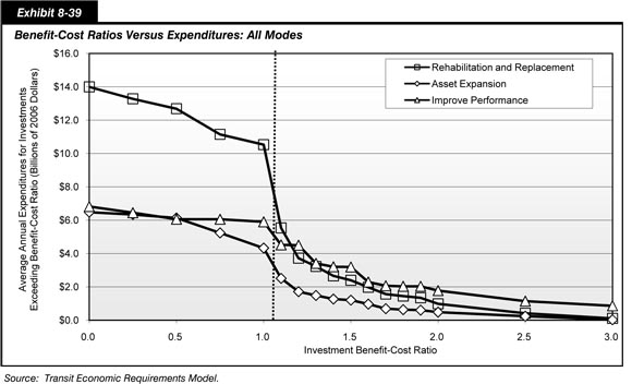
Comparison
The layout and content of Part II of this edition of the C&P report, including Chapters 7 through 10, has been restructured significantly relative to that of recent editions. Much of the material presented in this chapter represents extensions to more limited analyses presented in Chapters 7, 8, 11, and 12 of the 2006 C&P Report. This discussion of selected capital investment scenarios was moved to Chapter 8 in this report to allow it to follow the more detailed technical analysis presented in Chapter 7, and to emphasize the fact that these scenarios represent only selected points on a broad continuum of possible future investment levels.
| What is the Federal share of the highway and transit investment scenario estimates presented in this report? | |
|
The investment scenario estimates presented in this report represent the projected levels of total capital investment that would be necessary to obtain certain outcomes. The question of what portion should be funded by the Federal government, State governments, local governments, or the private sector is outside the scope of this report.
Chapter 6 includes information on historic trends in public funding for highways and transit by different levels of government.
|
|
Exhibits 8-40 and 8-41 summarize the average annual investment levels associate with each of the highway and transit investment scenarios presented in the highway and transit sections of this chapter, respectively. These exhibits also compare these investment levels with actual combined public and private highway capital investment in 2006. The scenarios can mainly be classified into two broad categories, those focused on maintaining selected indicators of system conditions and performance, and those focused on improving the overall conditions and performance of the system.
| Scenario Description | Average Annual Investment (Billions of 2006 Dollars) Interstate |
Average Annual Investment (Billions of 2006 Dollars) NHS |
Average Annual Investment (Billions of 2006 Dollars) All Roads |
Percent Difference Relative to 2006 Spending Interstate |
Percent Difference Relative to 2006 Spending NHS |
Percent Difference Relative to 2006 Spending All Roads |
Annual Percent Increase to Support Scenario Investment 1 Interstate |
Annual Percent Increase to Support Scenario Investment 1 NHS |
Annual Percent Increase to Support Scenario Investment 1 All Roads |
|---|---|---|---|---|---|---|---|---|---|
| Scenarios Assuming Fixed Rate User Financing | |||||||||
| Sustain Current Spending | $16.5 | $37.1 | $78.7 | 0.0% | 0.0% | 0.0% | 0.00% | 0.00% | 0.00% |
| Sustain Conditions and Performance | $24.8 | $38.7 | $105.6 | 49.8% | 4.4% | 34.2% | 3.71% | 0.41% | 2.72% |
| Invest up to MinBCR=1.5 | $39.0 | $60.7 | $137.4 | 135.7% | 63.7% | 74.6% | 7.61% | 4.49% | 5.05% |
| Invest up to MinBCR=1.2 | $43.5 | $69.2 | $157.1 | 163.1% | 86.5% | 99.7% | 8.52% | 5.62% | 6.21% |
| Invest up to MinBCR=1.0 | $47.0 | $76.1 | $174.6 | 183.9% | 105.1% | 121.9% | 9.15% | 6.43% | 7.10% |
| Sustain Conditions and Performance of System Components | N/A | N/A | $119.5 | N/A | N/A | 51.9% | N/A | N/A | 3.83% |
| Sustain Conditions and Improve Performance | N/A | N/A | $143.5 | N/A | N/A | 84.7% | N/A | N/A | 5.54% |
| Scenarios Assuming Variable Rate User Financing | |||||||||
| Sustain Current Spending | $16.5 | $37.1 | $78.7 | 0.0% | 0.0% | 0.0% | 0.00% | 0.00% | 0.00% |
| Sustain Conditions and Performance | $11.6 | $19.6 | $71.3 | -29.7% | -47.0% | -9.3% | -3.49% | -6.54% | -0.94% |
| Invest up to MinBCR=1.5 | $24.0 | $38.9 | $101.8 | 45.3% | 4.9% | 29.5% | 3.43% | 0.46% | 2.40% |
| Invest up to MinBCR=1.2 | $27.5 | $44.9 | $117.2 | 66.5% | 21.2% | 48.9% | 4.64% | 1.80% | 3.65% |
| Maximum Economic Investment (MinBCR=1.0) | $30.4 | $50.1 | $131.3 | 83.8% | 35.3% | 66.9% | 5.49% | 2.79% | 4.66% |
| Sustain Conditions and Performance of System Components | N/A | N/A | $83.4 | N/A | N/A | 6.0% | N/A | N/A | 0.55% |
| Sustain Conditions and Improve Performance | N/A | N/A | $104.9 | N/A | N/A | 33.4% | N/A | N/A | 2.67% |
| Rehabilitation and Replacement Maintain |
Rehabilitation and Replacement Improve |
Asset Expansion | Performance Improvement | Total | |
|---|---|---|---|---|---|
| Maintain Current Funing | |||||
| 2006 Funding Levels | $9.3 | $9.3 | $2.4 | $1.1 | $12.8 |
| Traditional TERM Scenarios | |||||
| Maintain Conditions and Performance BCR=1.0 | $10.7 | N/A | $4.3 | N/A | $15.1 |
| Improve Conditions and Performance BCR=1.0 | N/A | $12.2 | $2.9 | $5.9 | $21.1 |
| Benefit-Cost Ratio Increased to 1.2 | |||||
| Maintain Conditions and Performance BCR=1.2 | $3.9 | N/A | $1.7 | N/A | $5.6 |
| Improve Conditions and Performance BCR=1.2 | N/A | $4.1 | $1.5 | $4.5 | $10.2 |
| Congestion Pricing Scenarios | |||||
| Maintain Conditions and Performance BCR=1.0, SCS 25% | $10.9 | N/A | $7.8 | N/A | $18.7 |
| Improve Conditions and Performance BCR=1.0, SCS 25% | N/A | $11.3 | $7.8 | $5.9 | $25.0 |
| Maintain Conditions and Performance BCR=1.2, SCS 25% | $4.9 | N/A | $4.0 | N/A | $8.3 |
| Improve Conditions and Performance BCR=1.2, SCS 25% | N/A | $4.0 | $3.5 | $4.5 | $11.9 |
| Maintain Conditions and Performance BCR=1.0, MEI 25% | $10.8 | N/A | $7.4 | N/A | $18.2 |
| Improve Conditions and Performance BCR=1.0, MEI 25% | N/A | $11.3 | $7.4 | $5.9 | $24.6 |
| Maintain Conditions and Performance BCR=1.2, MEI 25% | $4.8 | N/A | $3.2 | N/A | $8.0 |
| Improve Conditions and Performance BCR=1.2, MEI 25% | N/A | $5.3 | $3.2 | $4.5 | $13.0 |
| Maintain Conditions and Performance BCR=1.0, SCS 50% | $11.8 | N/A | $10.3 | N/A | $22.1 |
| Improve Conditions and Performance BCR=1.0, SCS 50% | N/A | $12.3 | $10.3 | $5.9 | $28.5 |
| Maintain Conditions and Performance BCR=1.2, SCS 50% | $8.6 | N/A | $7.8 | N/A | $16.4 |
| Improve Conditions and Performance BCR=1.2, SCS 50% | N/A | $9.2 | $7.8 | $4.5 | $21.4 |
| Maintain Conditions and Performance BCR=1.0, MEI 50% | $11.8 | N/A | $10.6 | N/A | $22.4 |
| Improve Conditions and Performance BCR=1.0, MEI 50% | N/A | $12.3 | $10.6 | $5.9 | $28.8 |
| Maintain Conditions and Performance BCR=1.2, MEI 50% | $8.3 | N/A | $7.2 | N/A | $15.6 |
| Improve Conditions and Performance BCR=1.2, MEI 50% | N/A | $8.0 | $7.2 | $4.5 | $20.5 |
For highways and bridges, the Sustain Conditions and Performance scenario focuses on maintaining the system at base year performance levels. The MinBCR=1.5, MinBCR=1.2, and MinBCR=1.0 scenarios represent three alternative levels of investment that would each improve the performance of the overall system by varying degrees. A Sustain Current Spending scenario was included to project the impact that maintaining combined public and private highway capital spending at base year levels would be expected to have on system conditions and performance. Separate versions of each scenario were developed assuming either fixed rate user financing or variable rate user financing would be utilized to support the overall level of investment associated with that scenario. Each scenario was also computed separately for the Interstate system and the National Highway System, as well as for the overall network of highways and bridges as a whole. Two supplemental highway and bridge scenarios were presented at the systemwide level only. The Sustain Conditions and Performance of System Components scenario represents an alternative approach to maintaining the system; the Sustain Conditions and Improve Performance scenario focuses on maintaining physical conditions while improving operational performance.
For transit the Maintain Current Funding scenario considers the expected impact on the long-term physical condition and service performance of the Nation's transit infrastructure if current (2006) transit investment levels for rehabilitation, replacement, and expansion are maintained through the year 2026. The traditional TERM scenarios are consistent with the 2006 C&P Report. These scenarios estimate the level of investment required to: (1) Maintain transit asset physical conditions and service performance at current levels, or (2) Improve transit asset physical conditions and service performance to specific condition and performance targets. These scenarios represent all investments that pass the benefit-cost ratio at greater than or equal to 1.0. For the 2008 C&P Report, additional scenarios were included to demonstrate the effect on investments of shifting the benefit-cost ratio from 1.0 to 1.2. Congestion pricing scenarios were also included that examine the level of transit expansion investment required to serve highway users diverted to transit as a result of highway congestion pricing while maintaining current transit performance. Each of these scenarios was assessed with a benefit-cost ratio of 1.0, and then examined as the ratio shifts to 1.2.
Exhibit 8-42 compares selected 20-year average annual investment scenario estimates in this report with those presented in the 2004 C&P Report. The first column shows the projection for 2005 to 2024, based on 2004 data shown in the 2006 C&P Report and stated in 2004 dollars. The second column restates these highway and transit values in 2006 dollars, to account for the effect of inflation. The third column shows new average annual investment scenario projections for 2007 to 2026 based on 2006 data.
| Scenario | 2005–2024 Projection (Based on 2004 Data) 2006 Report (Billions of 2004 $) |
2005–2024 Projection (Based on 2004 Data) Adjusted for Inflation* (Billions of 2006 $) |
2007–2026 Projection (Based on 2006 Data) (Billions of 2006 $) |
|---|---|---|---|
| Highway and Bridge Scenarios—All Roads | |||
| Sustain Conditions and Performance Scenario Assuming Fixed Rate User Financing |
$78.8 | $112.9 | $105.6 |
| MinBCR=1.0 Scenario Assuming Fixed Rate User Financing |
$131.7 | $188.8 | $174.6 |
| Sustain Conditions and Performance Scenario Assuming Variable Rate User Financing | $57.2 | $82.0 | $71.3 |
| Maximum Economic Investment Scenario (MinBCR=1.0 Assuming Variable Rate User Financing) |
$110.8 | $158.8 | $131.3 |
| Transit Scenarios (BCR=1.0) | |||
| Maintain Conditions and Performance | $15.8 | $17.3 | $15.1 |
| Improve Conditions and Maintain Performance | $16.4 | $18.0 | $15.2 |
| Maintain Conditions and Improve Performance | $21.2 | $23.2 | $21.0 |
| Improve Conditions and Performance | $21.8 | $23.9 | $21.1 |
For transit, the ENR Building Construction Index, 2000 to 2008, was utilized.
Highways and Bridges
As discussed in Chapter 6, highway construction costs as measured by the Federal Highway Administration Composite Bid Price Index (BPI) increased by 43.3 percent from 2004 to 2006. This increase had a significant impact on the capital investment scenarios presented in this report.
As shown in Exhibit 8-42, the $105.6 billion average annual investment level in constant 2006 dollars for the version of the Sustain Conditions and Performance scenario assuming fixed rate user financing is significantly higher than the amount shown for the comparable "Cost to Maintain" scenario in the 2006 C&P Report, which was stated in constant 2004 dollars; however, accounting for inflation this new estimate is actually 6.5 percent lower in constant dollar terms. Similarly, assuming fixed rate user financing, the $174.6 billion average annual investment level under the MinBCR=1.0 scenario stated in constant 2006 dollars is significantly higher than the amount shown in 2004 dollars for the "Cost to Improve" scenario in the 2006 C&P Report. However, accounting for inflation, this new estimate for the 2007 to 2026 period is actually 7.5 percent lower in constant dollar terms than the projection for the 2005 to 2024 period reflected in the 2006 C&P Report. Due to the increase in construction costs, some potential projects that might have been considered cost-beneficial in the previous 2006 C&P Report would not longer meet that standard; however, those projects that would be implemented under this scenario would each be more expensive than was assumed in the 2006 C&P Report, adding to the costs associated with this scenario.
Exhibit 8-42 also shows the variable rate user financing versions of these two scenarios with values presented in sensitivity analyses shown in Chapter 10 of the 2006 C&P Report, that were generally comparable to the scenarios presented in this chapter. The $71.3 billion average annual investment level in constant 2006 dollars for the version of the Sustain Conditions and Performance scenario assuming variable rate user financing is significantly higher than the amount shown for the comparable 2004 dollar "Cost to Maintain" value shown in the 2006 C&P Report; however, accounting for inflation this new estimate is actually 13.0 percent lower in constant dollar terms. Assuming variable rate user financing, the $131.3 billion average annual investment level under the Maximum Economic Investment (MinBCR=1.0) scenario stated in constant 2006 dollars is significantly higher than the comparable "Cost to Improve" figure presented in the 2006 C&P Report, stated in 2004 dollars. However, accounting for inflation, this new estimate for the 2007 to 2026 period is actually 17.3 percent lower in constant dollar terms than the projection for the 2005 to 2024 period reflected in the 2006 C&P Report.
The changes in the projected investment scenario levels from the 2006 C&P Report are also partially attributable both to changes in the underlying characteristics, conditions, and performance of the highway system as reported in the available data sources, and to changes in the methodology and models used to generate the estimates. In addition to the inflation adjustments noted above, the highway improvement costs estimates in HERS were updated to reflect better information regarding costs associated with projects in large urbanized areas. These new estimates, which are generally higher than those used previously, reflect the increasing complexity of implementing highway projects in large cities, which often require additional costs aimed at mitigating the impacts of improvements on the environment, communities, and current users of the roadways. Appendix A discusses other recently methodological improvements to HERS.
Exhibit 8-43 compares the estimated percentage differences between current spending and the average annual investment scenario estimates for the fixed rate user financing versions of Sustain Conditions and Performance scenario and the MinBCR=1.0 scenario and with the values reported for the primary "Maintain" and "Improve" scenarios identified in the 1997, 1999, 2002, 2004, and 2006 C&P Reports.
| Report Year | Relevant Comparison | Percent Above Current Spending Primary "Maintain" Scenario* |
Percent Above Current Spending Primary "Improve" Scenario* |
|---|---|---|---|
| 1995 | Average annual investment scenario estimates for 1994–2013 compared with 1997 spending | 57.5% | 112.6% |
| 1997 | Average annual investment scenario estimates for 1996–2015 compared with 1995 spending | 21.0% | 108.9% |
| 1999 | Average annual investment scenario estimates for 1998–2017 compared with 1997 spending | 16.3% | 92.9% |
| 2002 | Average annual investment scenario estimates for 2001–2020 compared with 2000 spending | 17.5% | 65.3% |
| 2004 | Average annual investment scenario estimates for 2003–2022 compared with 2002 spending | 8.3% | 74.3% |
| 2006 | Average annual investment scenario estimates for 2005–2024 compared with 2004 spending | 12.2% | 87.4% |
| 2008 | Average annual investment scenario estimates for 2007–2026 compared with 2006 spending | 34.2% | 121.9% |
The recent increases in highway construction costs have caused the percentage difference between current capital spending and the fixed rate user financing versions of Sustain Conditions and Performance scenario to grow to 34.2 percent, which is the higher the comparable figures identified in recent editions, though it is lower than the 57.5 percent gap identified for the comparable "Maintain" scenario in the 1995 C&P Report. The 121.9 percent difference between the current spending and the MinBCR=1.0 scenario has also increased sharply from the comparable figures presented in recent reports. Note that the variable rate financing versions of these two scenarios show much smaller gaps; as shown in Exhibit 8-40 the difference between current spending and the Maximum Economic Investment (Min BCR=1.0) scenario is only 66.9 percent, while average annual investment for the Sustain Conditions and Performance scenario is actually 9.3 percent lower than base year spending.
Transit
As shown in Exhibit 8-42, for Maintain Conditions and Performance, the updated annual investment requirement projection for 2007 to 2026 of $15.1 billion per year is significantly less than the inflation adjusted amount of $17.3 billion from the 2006 C&P Report for 2005 to 2024. This trend continues with the Improve Conditions and Maintain Performance scenario, which compares a current estimate of a $15.2 billion per year investment requirement to an estimate of $18.0 billion per year in the 2006 C&P Report (both reported in 2006 dollars). Maintain Conditions and Improve Performance and Improve Conditions and Performance are more consistent with the estimates provided in the 2006 Report. However, when adjusted for inflation, the analyses presented in this report are again less than the estimates in 2006 dollars. These downward trending changes to projected annual investment requirements as compared to the 2006 C&P Report were driven primarily by updates to the available data through the National Transit Database as well as changes in the methodology used by the Transit Economic Requirements Model.
Exhibit 8-44 compares the percentage difference between current capital spending levels and the level of transit investment estimated by TERM in 2006 with the percentage difference between capital spending levels and the projected investment estimates from TERM provided in previous years C&P reports. As a result of methodological improvements, the TERM projections are not directly comparable from year to year. The annual amount of investment estimated by TERM to maintain conditions and performance between 2007 and 2026 is 28.2 percent higher than actual capital expenditures in 2006. In the 2006 C&P Report, the amount of annual investment estimated by TERM to maintain conditions and performance from 2005 to 2024 was 25.4 percent higher than actual capital expenditures in 2004. This comparison between actual spending and TERM projections had historically presented the TERM projections declining as a percentage difference to actual spend. This edition shows a larger gap between investment levels and current spending than was indicated in previous reports.
| Report Year | Spending Year | Investment Forecast Years | Percent Above Current Spending Cost to Maintain Conditions and Performance |
Percent Above Current Spending Cost to Improve Conditions and Performance |
|---|---|---|---|---|
| 1995 | 1993 | 1994–2013 | 37.6% | 124.4% |
| 1997 | 1995 | 1996–2015 | 38.3% | 102.9% |
| 1999 | 1997 | 1998–2017 | 41.0% | 110.2% |
| 2002 | 2000 | 2001–2020 | 63.8% | 127.7% |
| 2004 | 2002 | 2003–2022 | 26.8% | 95.1% |
| 2006 | 2004 | 2005–2024 | 25.4% | 73.0% |
| 2008 | 2006 | 2007–2026 | 28.2% | 64.1% |