Executive Summary

Chapter 1

An Introduction to Highways and Transit

Highways and public transit in the U.S. form the foundation for one of the most extensive and complicated transportation networks in the world.

The Essential Functions of Highway and Transit Infrastructure

There are several ways that highways and transit interact to provide service for the American people.

First, highways and transit provide the American people with a high degree of personal mobility. Many of the Nation's social, governmental, and legal principles were built around the concept of freedom of movement.

Second, the Nation's surface transportation system plays an essential role in moving freight. Most goods are moved by truck over the Nation's highways. By reducing traffic volume, transit can reduce congestion and free up highway capacity for freight movement.

Third, transportation plays an essential role in the economic viability of communities. Highway and transit corridors support commerce and employment and allow cities to target investment in areas that best promote livable and sustainable urban development. Property values are higher in areas with the best access to transportation.

Fourth, highways and transit systems play an important role in protecting the American public. The Nation's highway system is essential for much of the Nation's military mobilization. Highways must also be able to quickly accommodate police, fire, and rescue vehicles. Both highways and transit can help evacuate cities when there are emergencies.

The Complementary Role of Highways and Transit

Highways and transit are complementary, serving distinct but overlapping markets in the Nation's transportation system. An efficient transit system gives people living in dense, urban environments increased mobility. An effective highway system does the same for people in suburban or rural areas.

Highway investments can benefit those transit modes that share roadways with private automobiles, such as buses, vanpools, and demand response vehicles. Having good highway access to transit stations in outlying areas, meanwhile, increases accessibility to transit.

Transit improvements can enhance the operational performance of highways by attracting private vehicle drivers off the road during peak periods of congestion.

Public and private assets also complement one another. Although the Nation's highways are typically publicly owned, many people use the system through privately owned automobiles. Transit is generally provided by public agencies, either directly or through private contractors.

Chapter 2

System Characteristics: Highways and Bridges

In 2006, a network of 4.03 million miles of public roads provided mobility for the American people. (The terms "roads" and "highways" are used interchangeably in this report). Rural areas accounted for 74.2 percent of this mileage. While urban mileage constitutes only 25.8 percent of total mileage, these roads carried 66.3 percent of the 3.0 trillion vehicle miles traveled (VMT) in the United States in 2006. In 2006, there were 597,562 bridges throughout the Nation; 75.5 percent of these were in rural areas.

Rural local roads made up 50.8 percent of total mileage, but carried only 4.3 percent of total VMT. In contrast, urban Interstate highways made up only 0.4 percent of total mileage but carried 16.3 percent of total VMT.

Percentage of Highway Miles, Bridges, and Vehicle Miles
Traveled by Functional System, 2006

Functional System	Miles	Bridges	VMT
Rural Areas
Interstate	0.8%	4.5%	8.4%
Other Principal Arterial	2.4%	6.0%	7.5%
Minor Arterial	3.4%	6.6%	5.3%
Major Collector	10.4%	15.7%	6.3%
Minor Collector	6.5%	8.1%	1.9%
Local	50.8%	34.7%	4.3%
Subtotal Rural	74.2%	75.5%	33.7%
Urban Areas
Interstate	0.4%	4.8%	16.3%
Other Freeway and Expressway	0.3%	3.0%	7.5%
Other Principal Arterial	1.6%	4.4%	15.4%
Minor Arterial	2.6%	4.4%	12.6%
Collector	2.7%	2.9%	5.8%
Local	18.3%	4.9%	8.8%
Subtotal Urban	25.8%	24.4%	66.3%
Total	100.0%	100.0%	100.0%

Total highway mileage increased at an average annual rate of 0.2 percent between 1997 and 2006, while total VMT grew at an average annual rate of 1.9 percent. Rural road mileage has declined since 1997, due in part to the reclassification of some Federal roads as nonpublic and the expansion of urban area boundaries as a result of the decennial Census. Urban areas are defined to include all places with a population of 5,000 or greater; all other locations are classified as rural.

Rural VMT grew at an average annual rate of 0.4 percent from 1997 to 2006, compared with an average annual increase of 1.7 percent in small urban areas (population 5,000 to 50,000) and 2.9 percent in urbanized areas.

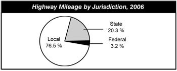
In 2006, 76.5 percent of highway miles were locally owned, 20.3 percent were owned by States, and 3.2 percent were owned by the Federal government. The share of locally owned roads grew slightly between 1997 and 2006, increasing from 75.3 percent. During that same period, the share of State-owned mileage remained mostly constant and Federally owned road mileage decreased from 4.3 percent in 1997 to 3.2 percent in 2006.

In 2006, 50.5 percent of bridges were locally owned, 47.6 percent were owned by States, 1.4 percent were owned by the Federal government, and 0.5 percent were either privately owned (including highway bridges owned by railroads) or had unknown or unclassified owners. About 46.8 percent of all bridges were built before 1966.

The 163,462-mile National Highway System (NHS) includes the Nation's key corridors and carries much of its traffic. In 2006, NHS included only 4.0 percent of the Nation's total route mileage, but its roads carried 44.6 percent of VMT.

The Interstate System is the core of NHS and includes the most-traveled routes. All Interstates are part of the NHS, as are 83.5 percent of rural other principal arterials, 87.2 percent of urban other freeways and expressways, and 36.3 percent of urban other principal arterials. Interstate travel represented the fastest-growing portion of VMT between 1997 and 2006.

Chapter 2

System Characteristics: Transit

Transit system coverage, capacity, and use in the United States continued to increase between 2004 and 2006. In 2006, there were 657 agencies in urbanized areas reporting to the National Transit Database (NTD), of which 588 were public agencies, including seven State Departments of Transportation. Of the 657 reporting agencies, 83 received either a temporary reporting waiver or a reporting exemption for operating nine or fewer vehicles. The remaining 575 reporting agencies provided service on 1,398 different modal networks; 162 agencies operated a single mode and 495 transit agencies operated more than one mode. In 2006, there were an additional 1,327 transit operators serving rural areas.

In 2006, urban transit systems, excluding special service providers, operated 128,132 vehicles compared with 120,659 vehicles in 2004, an increase of 6.2 percent. In 2006, transit providers operated 11,796 miles of track and served 3,053 stations, compared with 10,892 miles of track and 2,961 stations in 2004. In 2006, there were 813 maintenance facilities for all transit modes in urban areas, compared with 793 in 2004. In 2006, the first year for which rural data are available through the NTD, there were 1,327 rural transit operators, a significant increase over 1,215 in 2000. In 2006, 80 percent of all transit vehicles reported to the NTD were compliant with the Americans with Disabilities Act (ADA). In 2006, 72 percent of total transit stations were ADA-compliant.

In the United States in 2006, 223,489 urban route miles were provided by nonrail modes, which is consistent with 2004 data (at 216,619 urban route miles). Rail modes provided 10,865 urban route miles, an increase from 9,782 in 2004.

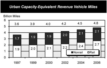
For all modes, capacity-equivalent vehicle revenue miles (VRMs) increased at an average annual rate of 3.5 percent between 1997 and 2006 and 3.5 percent between 2004 and 2006. Rail capacity-equivalent VRMs provided 2.7 billion capacity-equivalent miles, and nonrail provided 2.1 billion miles in 2006.

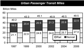
Transit passenger miles traveled (PMT) increased by 6.4 percent between 2004 and 2006, from 46.5 billion to 49.5 billion. PMT traveled on nonrail modes increased from 20.9 billion to 22.5 billion, or 7.9 percent. PMT on rail transit modes increased from 25.7 billion in 2004 to 27.0 billion in 2006, or by 5.1 percent.

Approximately 56.2 percent of unlinked trips were on motor buses, 31.2 percent were on heavy rail, 4.7 percent were on commuter rail, 4.3 percent on light rail, and 3.5 percent categorized as other. By comparison, 41.2 percent of PMT in 2006 were on motor bus, 29.7 percent were on heavy rail, 20.9 percent were on commuter rail, and 3.8 and 4.4 percent respectively were on light rail and other. Percentages across modes can differ as average trip length can vary by mode. While unlinked passenger trips and PMT both increased by approximately 6 percent, the allocation across the modes remained relatively unchanged.

Chapter 3

System Conditions: Highways and Bridges

Poor pavement condition imposes economic costs on highway users in the form of increased wear and tear on vehicle suspensions and tires, delays associated with vehicles slowing to avoid potholes, and crashes resulting from unexpected changes in surface conditions. While transportation agencies consider many factors when assessing the overall condition of highways and bridges, surface roughness most directly affects the ride quality experienced by drivers.

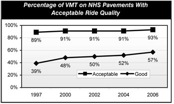
On NHS, the percentage of VMT on pavements with good ride quality has risen sharply over time, from approximately 39 percent in 1997 to about 57 percent in 2006. The VMT on NHS pavements meeting the acceptable standard of ride quality grew more slowly, from approximately 89 percent in 1997 to approximately 93 percent in 2006.

Rural NHS routes tend to have better pavement conditions than urban NHS routes. In 2006, for example, about 98 percent of all VMT on rural pavements was traveled on routes with acceptable ride quality. By contrast, the portion of urban NHS VMT on acceptable pavements was 90 percent that same year.

For Federal-aid highways as a whole, including the NHS and other arterials and collectors eligible for Federal funding, the VMT on pavements with good ride quality increased from 39.4 percent in 1997 to 47.0 percent in 2006. The VMT on pavements meeting the less stringent standard of acceptable ride quality decreased slightly from 86.4 percent in 1997 to 86.0 percent.

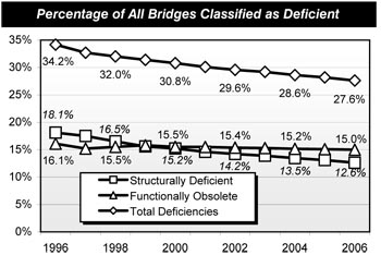
Most bridges are inspected every 24 months and receive ratings based on the condition of various bridge components. Two terms used to summarize bridge deficiencies are "structurally deficient" and "functionally obsolete." Structural deficiencies are characterized by deteriorated conditions of significant bridge elements and reduced load-carrying capacity. A "structurally deficient" designation does not imply that a bridge is unsafe, but such bridges typically require significant maintenance and repair to remain in service, and would eventually require major rehabilitation or replacement to address the underlying deficiency. A bridge is considered functionally obsolete when it does not meet current design standards, either because the volume of traffic carried by the bridge exceeds the level anticipated when the bridge was constructed and/or the relevant design standards have been revised. Addressing functional deficiencies may require the widening or replacement of the structure. Rural bridges tend to have a higher percentage of structural deficiencies, while urban bridges have a higher incidence of functional obsolescence due to rising traffic volumes.

The share of bridges classified as deficient fell from 34.2 percent in 1996 to 27.6 percent in 2006. Most of this decline was the result of reductions in the percent of structurally deficient bridges.

Chapter 3

System Conditions: Transit

The overall physical condition of the U.S. transit system can be evaluated by examining the age and condition of the various components of the Nation's infrastructure. This infrastructure includes vehicles in service, maintenance facilities, the equipment they contain, and other supporting infrastructure such as guideways, power systems, rail yards, stations, and structures (bridges and tunnels). Since the 2006 C&P Report, asset data for approximately 71 percent of the Nation's transit assets have been updated.

Definitions of Transit Asset Conditions

Rating	Condition	Description
Excellent	5	No visible defects, near new condition.
Good	4	Some slightly defective or deteriorated components.
Adequate	3	Moderately defective or deteriorated components.
Marginal	2	Defective or deteriorated components in need of replacement.
Poor	1	Seriously damaged components in need of immediate repair.

The Federal Transit Administration (FTA) has undertaken extensive engineering surveys and collected a considerable amount of data on the U.S. transit infrastructure to evaluate transit asset conditions. FTA uses a rating system of 1, "poor," to 5, "excellent," to describe asset conditions. The Rail Modernization study, released by FTA in April 2009, considered an asset to be in a state of good repair when the physical condition of that asset is at or above a specific condition rating value of 2.5 (the mid-point between adequate and marginal). This replaces the over-age criteria used in previous C&P reports, which were based on FTA's minimum vehicle replacement ages.

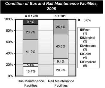
The estimated average condition rating of urban bus vehicles declined slightly from a rating of 3.08 in 2004 to 3.01 in 2006. The average age of urban bus vehicles remained constant at 6.1 years, with 21.8 percent of the fleet considered over-age. The average estimated condition of bus maintenance facilities declined from 3.41 in 2004 to 3.26 in 2006. In 2006, 63.7 percent of bus maintenance facilities were in adequate, good, or excellent condition, a decline from 68.1 percent in 2004.

The estimated average condition rating of rail vehicles continued to increase from 3.50 in 2004 to 3.51 in 2006. The average age of rail vehicles remained relatively consistent at 19.8 years in 2006 compared with 19.7 years in 2004, with 32.1 percent of the fleet defined as over-age. The estimated average condition of rail maintenance facilities decreased from 3.82 in 2004 to 3.68 in 2006. In 2006, 73.8 percent of rail maintenance facilities were estimated to be in adequate, good, or excellent condition.

The estimated average condition rating of rail stations improved from 3.37 in 2004 to 3.53 in 2006. In 2006, 99.3 percent of communications systems, 80.2 percent of train control systems, and 88.5 percent of traction power systems were in adequate, good, or excellent condition. The estimated average conditions of elevated structures, underground tunnels, and track declined from 2004 and 2006; however, the condition of vehicle storage yards improved slightly.

The total value of the U.S. transit infrastructure was estimated at $607.2 billion in 2006. Of this total, rail assets comprise $500.8 billion, with nonrail and joint assets comprising the remaining $106.4 billion. The data collected for these efforts represent a significant improvement in data availability and are significantly more comprehensive in comparison to previous C&P reports.

Chapter 4

Operational Performance: Highways

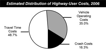
Americans continue to grapple with gridlock on the Nation's highways, leading to travel delays, wasted fuel, and billions of dollars in congestion costs. From an economic perspective, travel time accounts for almost half of all costs experienced by highway users (other key components of user costs include vehicle operating costs, and costs associated with crashes).

Congestion occurs when traffic demand approaches or exceeds the available capacity of the highway system. Three key aspects of congestion are severity, extent, and duration. Severity refers to the magnitude of the problem at its worst. The extent of congestion is the geographic area or number of people affected. Duration of congestion is the length of time that the traffic is congested.

Since there is no universally accepted definition of exactly what constitutes a congestion "problem," this report uses several metrics to explore different aspects of congestion.

The Texas Transportation Institute (TTI) collects data for 437 urban communities of different sizes across the Nation. The TTI 2007 Urban Mobility Report estimates that drivers experienced over 4.2 billion hours of delay and wasted approximately 2.9 billion gallons of fuel in 2005. The total congestion cost for these areas was $78.2 billion.

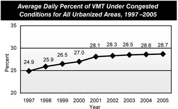
The average daily percentage of VMT under congested conditions is a metric that indicates the portion of daily traffic on freeways and other principal arterials in an urbanized area that moves at less than free-flow speeds. The measure increased by 3.8 percentage points from 24.9 percent in 1997 to 28.7 percent in 2005 for all urbanized areas combined. However the increase between 2004 and 2005 was only 0.1 percentage point, which suggests the growth of congestion is slowing. The largest increase during this period was in medium-sized urbanized areas with population between 500,000 and 999,999.

Another metric, the Travel Time Index, measures the amount of additional time required to make a trip during the congested peak travel period. Using the year 1987 as the base for comparison, the Travel Time Index for all urbanized areas increased from 1.16 to 1.28 in 2005. In 1997, a trip that would take 20 minutes during off-peak non-congested periods would take 4.6 minutes longer during the peak period. The same trip in 2005 would require 25.6 minutes during the peak period. The largest increase between 1997 and 2005 was experienced in medium-sized urbanized areas.

Travel Time Index by Urbanized Area Size, 1997–2005

Urbanized Area Population	Base Year 1987	Year 1997	Year 2005
Less Than 500,000	1.04	1.09	1.13
500,000 to 999,999	1.09	1.15	1.21
1,000,000 to 3,000,000	1.15	1.21	1.27
Over 3,000,000	1.26	1.33	1.40
All Urbanized Areas	1.16	1.23	1.28

The measure of annual hours of delay per capita represents the average amount of time lost due to congested conditions per urbanized area resident. The annual person-hours of delay per capita for all urbanized areas grew from 17.1 hours in 1997 to 21.8 hours in 2005.

The average length of congested conditions is a measure of the amount of time during a 24-hour period when traffic is operating under congested conditions. The average congested travel period increased from 5.9 hours in 1997 to 6.4 hours in 2005, although it has stabilized since 2002.

Chapter 4

Operational Performance: Transit

Transit operational performance can be measured and evaluated using a number of different factors, including the speed of passenger travel, vehicle utilization, and service frequency.

Average operating speed in 2006 remained consistent with 2004 levels at 20.0 miles per hour across all transit modes. Average operating speed is an approximate measure of the speed experienced by transit riders and is affected by dwell times and the number of stops. The average speed of nonrail modes was 14.4 miles per hour in 2006, improved from 14.0 miles per hour in 2004. Conversely, rail mode operating speeds decreased from 25.0 miles per hour in 2004 to 24.8 miles per hour in 2006.

Average vehicle occupancy levels increased across all rail and nonrail modes (excluding demand response and other rail) between 2004 and 2006 on an adjusted basis. The most significant increases were realized in light rail and ferryboat, at 7.5 and 9.0 percent, respectively.

Vehicle Utilization Passenger Miles
per Capacity-Equivalent Vehicle
(Thousands of Passenger Miles)

Mode	Utilization 2004	Utilization 2006
Commuter Rail	754.8	658.3
Heavy Rail	652.4	632.4
Vanpool	501.7	490.1
Light Rail	467.7	543.4
Motorbus	373.5	402.9
Ferryboat	328.4	287.8
Trolleybus	236.7	246.2
Demand Response	180.7	162.6

With the exception of light rail, motorbus and trolleybus, average vehicle utilization levels were lower in 2006 than in 2004. Vehicle utilization is measured as passenger miles per vehicle operated in maximum service, adjusted to reflect differences in the passenger-carrying capacities of transit vehicles. On average, rail vehicles operate at a higher level of utilization than nonrail vehicles. Commuter rail has consistently had the highest vehicle utilization rate, and demand response the lowest.

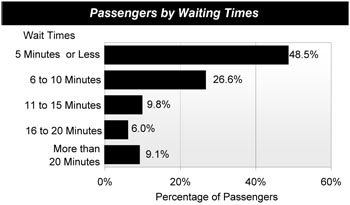
Most passengers who ride transit wait in areas that have frequent service. The 2001 National Household Travel Survey found that 49 percent of all passengers who ride transit wait for 5 minutes or less for a vehicle to arrive, and 75 percent wait 10 minutes or less. Nine percent of passengers wait for more than 20 minutes. To some extent, waiting times are correlated with incomes. Passengers with annual incomes above $65,000 are more likely to wait less time for a transit vehicle than passengers with incomes lower than $30,000. Higher-income passengers are more likely to be choice riders; passengers with lower incomes are more likely to use transit for basic mobility and to have more limited alternative means of travel.

Chapter 5

Safety: Highways

There has been considerable progress in reducing the number of highway fatalities since 1966, when Federal legislation first addressed highway safety. Since that time, the highest number of traffic deaths was 54,589 in 1972, while the lowest was 39,250 in 1992. Highway fatalities decreased from 42,836 in 2004 to 42,642 in 2006.

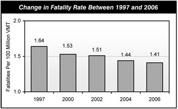
The fatality rate per 100 million vehicle miles traveled (VMT) has declined over time, as the number of VMT has increased. In 1966, the fatality rate per 100 million VMT was 5.50; this figure dropped to 1.64 in 1997, 1.44 in 2004, and 1.41 in 2006.

Fatality rates declined on every urban functional system between 1997 and 2006. Urban Interstate highways were the safest functional system, with a fatality rate of 0.55 per 100 million VMT in 2006. Urban minor arterials, however, recorded the sharpest decline in fatality rates. The fatality rate for urban minor arterials in 2006 was about 21.7 percent lower than in 1997.

There are many ways to examine the total number of highway-related crashes. One way is to look at roadway departure fatalities, where a vehicle leaves its lane and crashes. In 2006, there were 24,806 of these fatalities. About 43.1 percent involved the rollover of a passenger vehicle.

Another way is to examine fatalities that occur at intersections. Of the 42,642 fatalities that occurred in 2006, 19.6 percent—or 8,797—were related to intersections. Older drivers and pedestrians are particularly at risk at intersections. Half of the fatal crashes for drivers aged 80 or older and about one-third of the pedestrian deaths among people aged 70 or older occurred at intersections.

Another way to evaluate crashes is to analyze data related to crashes and fatalities caused by speeding. The National Highway Traffic Safety Administration estimates that 13,543 lives were lost in speed-related crashes in 2006.

Despite intense education and enforcement efforts, alcohol-impaired driving remains a serious public safety problem in the United States. In 2006, 17,602 Americans were killed in alcohol-related crashes on the Nation's highways. Alcohol was involved in 41 percent of fatal crashes and 9 percent of all crashes in 2006.

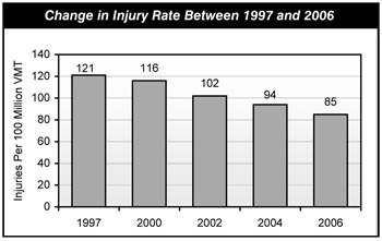
The overall number of traffic-related injuries has decreased over time, from about 3.4 million in 1988 to about 2.6 million in 2006. In 1988, the injury rate was 169 per 100 million VMT; by 2006, the number had dropped to 85 per 100 million VMT.

In terms of vehicle type, the number of occupant fatalities that involved passenger cars decreased from 22,199 in 1997 to 17,800 in 2006. Occupant fatalities involving light and large trucks, motorcycles, and other vehicles all increased.

In recent years, much attention has been focused on the safety of drivers at either extreme of the age spectrum. Motor vehicle crashes are the leading cause of death for Americans between the ages of 15 and 20 years old, and drinking is often a factor. Americans aged 65 and older, however, are among the safest drivers. They tend to be some of the most experienced drivers, and they are also less likely to drive while intoxicated.

Chapter 5

Safety: Transit

Public transit in the United States has been and continues to be a highly safe mode of transportation, as evidenced by the statistics on incidents, injuries, and fatalities that have been reported by transit agencies for the vehicles they operate directly. Reportable safety incidents include collisions and any other type of occurrence that results in death, a reportable injury, or property damage in excess of a threshold. Injuries and fatalities include those suffered by riders as well as by pedestrians, bicyclists, and people in other vehicles. Reportable security incidents include a number of serious crimes (robberies, aggravated assaults, etc.), as well as arrests and citations for minor offenses (fare evasions, trespassings, other assaults, etc.). Injuries and fatalities may occur not only while traveling on a transit vehicle, but also while boarding, alighting, or waiting for a transit vehicle or as a result of a collision with a transit vehicle or on transit property.

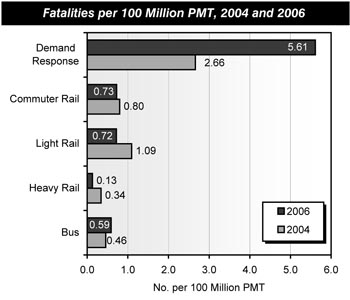
The definition of fatalities has remained the same. Fatalities decreased from 217 in 2004 to 213 in 2006, and fell from 0.52 per 100 million passenger miles travelled (PMT) in 2004 to 0.49 per 100 million PMT in 2006. Fatalities, adjusted for PMT, are lowest for heavy rail systems and motorbuses. Fatality rates for commuter and light rail have, on average, been higher than fatality rates for heavy rail. Commuter rail has frequent grade crossings with roads and shares track with freight rail vehicles; light rail is often at grade level and has minimal barriers between streets and sidewalks. Fatalities on demand response vehicles have consistently been the highest across all modes, increasing from 2.66 fatalities per 100 million PMT in 2004 to 5.61 in 2006.

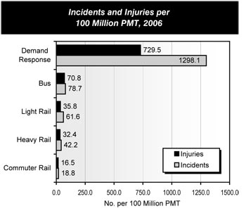
Incidents (safety and security combined) and injuries per 100 million PMT increased for all modes combined from 2004 to 2006. Incidents and injuries, when adjusted for PMT, are consistently the lowest for commuter rail and highest for demand response systems.

While commuter rail has a very low number of incidents per PMT, these incidents are more likely to result in a fatality than incidents occurring on any other mode at 3.85 fatalities per 100 incidents. Further, while light rail and motor bus have similar rates of incidents per PMT, an incident on light rail is more likely to produce a fatality (1.17 fatalities per 100 incidents for light rail compared with 0.75 for motor bus in 2006).

Chapter 6

Finance: Highways

In recent years, governments throughout the United States have experimented with new ways of financing transportation projects. As costs have increased, officials have often tried to replicate some of the most successful strategies of the private sector.

Public-Private Partnerships (PPPs) are increasingly applied to a large range of transportation functions across all modes. These functions may include project conceptualization, design, finance, construction, toll collection, and maintenance. Among the broad spectrum of PPP models, the most traditional is the private contract-fee services approach, where an agency transfers limited functions to a private company. In more advanced PPP models, a private company may control some or all of these functions through a lease of an asset over some period. Outright private ownership of highway assets remains rare.

Another innovative finance tool is the use of credit assistance. The Transportation Infrastructure Finance and Innovation Act of 1998 (TIFIA) provides Federal credit assistance for major transportation projects of national importance. So far, 17 projects have received commitments of TIFIA credit assistance. In addition, the State Infrastructure Bank Pilot Program offers direct loans and loan guarantees. As of June 2007, 33 States had taken advantage of this program.

Federal legislation has introduced additional ways to take advantage of debt financing. A Grant Anticipation Revenue Vehicle (GARVEE) generates up-front capital for major highway projects that the State may otherwise be unable to build in the near term. As of December 2007, the amount of GARVEE debt issued nationally had reached over $7.3 billion.

The trend toward tolling as an innovative finance technique has continued. Not only is there renewed emphasis on existing programs, such as the Congestion Pricing Pilot Program, but SAFETEA-LU also established several new innovative programs.

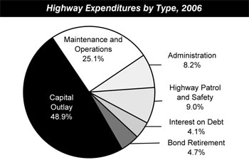
Governments throughout the United States spent $161.1 billion on highways in 2006. About $78.7 billion (48.8 percent) of this total was spent on capital projects. Another $40.4 billion was targeted toward maintenance (25.1 percent), while $14.5 billion (9.0 percent) was used for highway patrol and safety activities and $13.2 billion (8.2 percent) was spent on administrative costs; $14.2 billion (8.8 percent) was used for interest and bond retirement.

Of the $78.7 billion of capital spending in 2006, $40.4 billion was spent for rehabilitating the existing system; $16.2 billion was used to construct new roads and bridges; $13.8 billion was used for widening existing facilities; and $8.2 billion supported system enhancements such as safety, operational, and environmental enhancements. The portion of total capital outlay funded by the Federal government rose from 41.6 to 44.0 percent between 1997 and 2006; Federal support for capital projects climbed from $20.1 billion to $34.6 billion, while State and local capital investment increased from $28.3 billion to $44.1 billion. However, recent sharp increases in the prices of construction materials have reduced the purchasing power of this investment; in constant dollar terms, capital spending fell by 4.4 percent over this period.

In 2006, user charges including motor fuel taxes, motor-vehicle fees, and tolls were the source of 56.3 percent of all highway funding. The remaining 43.7 percent of revenues came from other sources, such as general fund appropriations, property taxes, assessments, and bond sales.

Chapter 6

Finance: Transit

In 2006, $43.4 billion was available from all sources to finance transit capital investments and operations, compared with $39.5 billion in 2004. Transit funding comes from public funds allocated by Federal, State, and local governments and system-generated revenues earned by transit agencies from the provision of transit services. In 2006, Federal funds accounted for 18.6 percent of all transit revenue sources, State funds for 19.7 percent, local funds for 33.0 percent, and system-generated funds for 28.7 percent.

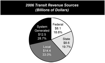
Eighty percent of the Federal funds allocated to transit are from a dedicated portion of the Federal motor-fuel tax receipts, and 20 percent are from general revenues. Federal funding for transit increased from $7.0 billion in 2004 to $8.1 billion, and State and local funding increased from $21.5 billion in 2004 to $22.8 billion in 2006.

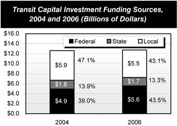
In 2006, $12.75 billion, or 29.4 percent of total available transit funds, was spent on capital investment. Federal capital funding was $5.6 billion, or 43.5 percent of total capital expenditures; State capital funding was $1.7 billion, or 13.3 percent of total capital expenditures; and local capital funding was $5.5 billion, or 43.1 percent of total capital expenditures. The share of those funding sources shifted slightly from 2004 to 2006, with Federal funds increasing to 43.5 percent from 39.0 percent in 2004, and local funding declining from 47.1 percent to 43.1 percent during that same time period.

In 2006, $4.5 billion (35.3 percent) of total capital expenditures was for guideway, $3.1 billion (24.3 percent) of the total was for rolling stock, and $2.2 billion (17.2 percent) of the total was for stations.

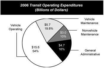
In 2006, actual operating expenditures were $29.0 billion. Vehicle operating expenses were $15.6 billion, 53.7 percent of total operating expenses and 35.9 percent of total expenses; vehicle maintenance expenses were $5.7 billion, 19.8 percent of total operating expenses and 13.2 percent of total expenses; nonvehicle maintenance expenses were $3.0 billion, or 10.4 percent of total operating expenses and 6.9 percent of total expenses; and general administrative expenses were $4.7 billion, or 16.2 percent of total operating expenses and 10.8 percent of total expenses.

In 2006, $30.6 billion was available for operating expenses, accounting for 70.6 percent of total available funds; the Federal government provided $2.5 billion, or 8.2 percent of total operating expenses; State governments $6.9 billion, or 22.5 percent of total operating expenses; local governments $8.9 billion, or 29.0 percent of total operating expenses; and system-generated revenues $12.3 billion, or 40.3 percent of total operating expenses.

Part II

Investment/Performance Analysis

Traditional engineering-based analytical tools focus mainly on estimating transportation agency costs and the value of resources required to maintain or improve the conditions and performance of infrastructure. This type of analytical approach can provide valuable information about the cost effectiveness of transportation system investments from the public agency perspective, including the optimal pattern of investment to minimize life-cycle costs. However, this approach does not fully consider the potential benefits to users of transportation services from maintaining or improving the conditions and performance of transportation infrastructure.

The investment/performance analyses presented in Chapters 7 through 10 of this report were developed using the Highway Economic Requirements System (HERS), the National Bridge Investment Analysis System (NBIAS), and the Transit Economic Requirements Model (TERM). Each of these tools has a broader focus than traditional engineering-based models and takes into account the value of services that transportation infrastructure provides to its users as well as some of the impacts that transportation activity has on non-users.

An economics-based approach will likely result in different decisions about the catalog of desirable improvements than would be made using a purely engineering-based approach. For example, if a highway segment, bridge, or transit system is greatly underutilized, benefit-cost analysis might suggest that it would not be worthwhile to fully preserve its condition or to address its engineering deficiencies. Conversely, a model based on economic analysis might recommend additional investments to expand capacity or improve travel conditions above and beyond the levels dictated by an analysis that simply minimized engineering life-cycle costs, if doing so would provide substantial benefits to the users of the system.

An economics-based approach also provides a more sophisticated method for prioritizing potential improvement options when funding is constrained. By identifying investment opportunities in order of the net benefits they offer, economic analysis helps provide guidance in directing limited resources toward those improvements that provide the largest benefits to transportation system users. Projects are ranked in order by their benefit-cost ratios, then successively implemented until the funding constraint is reached. Projects that produce lesser net benefits are deferred for reconsideration in the future.

For purposes of computing a benefit-cost ratio for a transportation project, the "costs" would reflect only the direct capital costs associated with that project. As defined in this report, the "benefits" would include reductions in costs of (1) transportation agencies (such as for maintenance), (2) users of the transportation system (such as savings in travel time or vehicle operating costs, or reductions in crashes), and (3) others who are affected by the operation of the transportation system (such as reductions in environmental or other societal costs). Increases in any of these costs would be treated as a negative benefit.

HERS, NBIAS, and TERM each use benefit-cost analysis as part of their decision-making process, but their approaches are very different. Each model relies on separate databases, making use of specific data available for only one part of the transportation network and addressing issues unique to that particular mode. The procedures for developing the investment scenario estimates have evolved over time, to incorporate new research, new data sources, and improved estimation techniques relying on economic principles. The methodologies used to analyze investment for highways, bridges, and transit are discussed in greater detail in Appendices A, B, and C.

While some new analysis has been added to this edition indirectly linking certain transit scenarios to specific highway scenarios involving shifts of peak period travelers between modes, the models have not evolved to the point where direct multimodal analysis is possible for the full range of scenarios.

Chapter 7 analyzes the projected impacts of different levels of future capital investment on a series of measures of physical condition, operational performance, and other benefits to system users. These levels are based on alternative annual rates of increase or decrease in constant dollar investment over 20 years.

The highway investment/performance analyses also examine the impacts of alternative financing mechanisms. Parallel analyses were constructed for each funding level assuming that any increases in investment above 2006 levels would be funded from non-user sources, user charges imposed on a fixed-rate per-mile basis (such as a VMT charge), or user charges imposed on a variable rate basis (such as congestion pricing). Any excess revenues stemming from decreases in highway and bridge investment below 2006 levels were assumed to be rebated to users in the form of reductions to existing fixed rate user charges.

Chapter 8 presents a set of illustrative 20-year capital investment scenarios building upon the analyses presented in Chapter 7. The Department does not endorse or recommend any particular scenario. Some of these scenarios are oriented toward maintaining different aspects of system conditions and performance, while others would improve the system to varying degrees. The investment levels associated with each scenario represent combined public and private capital spending; the scenarios do not identify how much might be contributed by each level of government to support such spending.

Chapter 9 provides supplemental analyses aimed at putting the scenarios presented in Chapter 8 into their proper context. It compares historic capital funding levels to recent conditions and performance trends and relates historic system use patterns to State and metropolitan planning organization (MPO) forecasts of future system use. The chapter also discusses the potential impacts of inflation, the timing of investments, and carbon dioxide emissions.

As in any modeling process, assumptions have been made in the models to make analysis practical and meet the limitations of available data. Chapter 10 explores the impact that varying some of these key assumptions would have on the overall results projected by HERS, NBIAS, and TERM. These include alternative assumptions regarding future deployments of operations technology, future levels of travel demand, the elasticity of travel demand to changes in user costs, future capital costs, discount rates, the valuation of nonmonetary benefits such as travel time savings, and the expected life span of pavements and structures.

While the economics-based approach applied in HERS, NBIAS, and TERM would suggest that projects be implemented in order based on their benefit-cost ratios (BCRs) until the funding available under a given scenario is exhausted, the reality is that other factors influence Federal, State, and local decisionmaking. If some projects with lower BCRs were carried out in favor of projects with higher BCRs, then the actual amount of investment required to achieve any given level of performance would be higher than the amount predicted in this report. Consequently, increasing spending to the level specified for one of the "maintain" scenarios would not guarantee that the targeted measures of conditions and performance would actually be sustained at base year levels.

Similarly, while the HERS, NBIAS, and TERM models all screen out potential improvements that are not cost-beneficial from the "improve" scenarios, simply increasing spending to the level associated with that scenario would not in itself guarantee that these funds would be expended in a cost-beneficial manner. There may also be some projects that, regardless of economic merits, may be infeasible as a practical matter due to factors beyond those considered in the models. Because of this, the supply of feasible cost-beneficial projects could be exhausted at a lower level of investment than indicated by these scenarios. Consequently, the improvements to future conditions and performance projected under the "improve" scenarios may not be fully obtainable in practice.

Chapter 7

Potential Capital Investment Impacts: Highways and Bridges

Chapter 7 explores the potential impacts of 24 alternative levels of future highway capital investment on various measures of conditions and performance. Each level is expressed as an annual percent change in constant dollar spending relative to 2006 levels. The NBIAS economic bridge investment backlog metric represents the level of potential bridge investments that would be cost-beneficial to implement. The HERS adjusted average highway user costs metric quantifies the impact that changes in system conditions and performance have on travel time costs (estimated to comprise 48.7 percent of total user costs in 2006), vehicle operating costs (35.0 percent), and crash costs (16.3 percent).

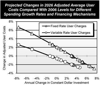
Of the $78.7 billion of total capital outlay in 2006, $48.2 billion was used for types of capital improvements modeled in HERS, including pavement resurfacing and reconstruction, and system expansion investments. Chapter 7 presents parallel analyses of alternative investment levels based on alternative financing mechanisms including funding from fixed rate user charges, and funding from variable rate user charges (direct pricing systems on congested highways).

Assuming variable rate user financing, adjusted average user costs are projected to decrease if spending were sustained at 2006 levels; if constant dollar spending were to decrease by 0.86 percent per year, this metric would still be sustained at 2006 levels through 2026. An increase of 4.55 percent per year in constant spending would yield a reduction in adjusted user costs of 5.1 percent; spending above this level would not be cost-beneficial. By 2026, each one percent reduction in user costs would translate into user savings of approximately $40 billion annually.

Regardless of the level of investment being analyzed, average user costs associated with fixed rate user financing would always be higher than if a variable rate user charge had been applied. Maintaining adjusted average user costs would require a 3.07 percent annual increase in spending assuming fixed rate user financing.

In 2006, $10.1 billion was spent by all levels of government on types of capital improvements modeled in NBIAS, including bridge repair, rehabilitation, and replacement actions. If combined public and private spending for the types of capital improvements modeled in NBIAS were sustained at 2006 levels in constant dollars, the economic bridge investment backlog is projected to rise from an initial level of $98.9 billion to a level of $112.6 billion, stated in 2006 dollars. This metric could be maintained at the 2006 base year level assuming annual spending growth of 0.83 percent per year in constant dollar terms; eliminating the backlog would require a 5.15 percent annual increase in constant dollar expenditures.

Chapter 7

Potential Capital Investment Impacts: Transit

Chapter 7 analyzes how different types and levels of annual capital spending would affect different future measures of transit system condition and performance.

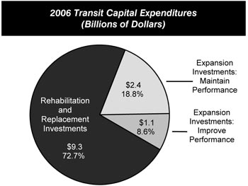
U.S. transit agencies spent $9.3 billion in 2006 to rehabilitate and replace antiquated and/or worn equipment. To maintain current average transit asset conditions into the future, providers of transit services would need to spend $11.4 billion annually on rehabilitation and replacement projects. (Note that this estimate is not comparable to the estimate shown in Chapter 8 because it includes capital investments in safety and other forms of capital spending not modeled by the Transit Economic Requirements Model [TERM].)

Transit operators expended $2.4 billion in 2006 on investments intended to maintain existing performance levels. If continued annually, this level of expenditure would cause crowding on transit vehicles to increase. To maintain current performance levels, U.S. transit operators would need to allocate $4.3 billion on performance maintenance (asset expansion) investments on a yearly basis.

In an effort to improve existing performance levels, U.S. transit agencies expended $1.1 billion in 2006. To improve performance through 2026, as defined by TERM, providers of transit services would need to increase annual capital spending on performance improving investments to $6.1 billion.

In addition to reviewing investment needs on a national basis, Chapter 7 identifies capital spending requirements for different segments of urbanized areas.

In large urbanized areas with heavy rail transit systems, transit agencies collectively spent $6.5 billion on rehabilitation and replacement investments in 2006. To maintain average conditions into the future, agencies in these cities would need to spend $8.0 billion annually. Agencies in large urbanized areas without heavy rail transit systems jointly spent $1.3 billion on these types of investments but would need to spend $1.6 billion annually to maintain average conditions. Finally, public transportation service providers in small cities and rural areas invested $0.7 billion rehabilitating and replacing transit assets. These agencies, however, would need to increase capital spending to $1.3 billion to maintain existing conditions.

Transit agencies also make investments intended to accommodate growth in demand for transit services.

Agencies operating in large metropolitan areas with heavy rail transit systems spent $0.2 billion in 2006 to expand service capacity. To keep pace with demand, however, agencies in these cities would need to increase capital expenditures on service-expanding investments to $3.3 billion annually.

In large cities without heavy rail transit systems, agencies invested $2.0 billion to expand capacity. If continued annually, this level of investment would allow agencies in these cities to maintain and even improve existing performance levels into the future.

Transit agencies in small cities and rural areas spent $0.1 billion to expand capacity in 2006. To maintain performance levels, however, agencies would need to increase annual capital spending on expansion projects to $0.3 billion.

Select analyses in this chapter include a Replace at Condition 2.5 scenario to help readers of the Rail Modernization Study that FTA released in April, 2009, place that study in the context of this report. The Rail Modernization Study considered seven select large transit rail agencies, a significant subset of the large urbanized areas with heavy rail transit systems discussed in this chapter.

Chapter 8

Selected Highway Capital Investment Scenarios

Chapter 8 presents a set of illustrative highway capital investment scenarios, building on the HERS and NBIAS analyses presented in Chapter 7, and taking into account other types of capital spending that are not currently modeled. The scenario criteria were applied separately to the Interstate System, the NHS, and the highway system as a whole. For each scenario, there is one version that assumes funding would be derived solely from fixed rate user based sources, and another that assumes funding would come from variable rate user based sources such as congestion pricing. This report does not endorse any of these scenarios as a target level of funding, nor does it make any recommendations concerning future levels of Federal funding.

The Sustain Current Spending scenario assumes that capital spending is maintained in constant dollar terms at base year 2006 levels between 2007 and 2026. (In other words, spending would rise by exactly the rate of inflation over that period). Of the $78.7 billion spent by all levels of government for highway capital improvements in 2006, $16.5 billion was directed to the Interstate System and $37.1 billion was directed to the NHS.

The Sustain Conditions and Performance scenario assumes that capital investment gradually changes in constant dollar terms over 20 years to the point at which adjusted average user costs and the economic bridge investment backlog in 2026 are maintained at their base year 2006 levels. Assuming fixed rate user financing, the average annual investment levels associated with meeting these goals are estimated to be $24.8 billion for the Interstate System, $38.7 billion for the NHS, and $105.6 billion for all roads. Assuming variable rate user financing, the average annual investment levels under this scenario would be $11.6 billion for the Interstate System, $19.6 billion for the NHS, and $71.3 billion for all roads. These values are lower than the amounts currently being spent on these systems, as the analysis indicates that current spending would be more than adequate to maintain system conditions and performance if congestion charges were widely applied.

Three scenarios are presented that would improve overall system conditions and performance. The MinBCR=1.5 scenario assumes that investment gradually increases in constant dollar terms over 20 years up to the point at which all potential capital improvements with a benefit-cost ratio of 1.5 or higher are funded by 2026 and the economic backlog for bridge investment is reduced to zero. The MinBCR=1.2 and MinBCR=1.0 scenarios make the same assumptions, but apply benefit-cost ratio cutoffs of 1.2 and 1.0, respectively. Assuming fixed rate user financing, the average annual investment level for all roads for the MinBCR=1.5, MinBCR=1.2, and MinBCR=1.0 scenarios, respectively, were estimated to be $137.4 billion, $157.1 billion, and $174.6 billion; assuming variable rate user financing, the comparable levels would be $101.8 billion, $117.2 billion, and $131.3 billion. (The MinBCR=1.0 scenario is equivalent to the Cost to Improve Highways and Bridges described in previous editions of this report).

Summary of Selected Highway Capital Investment Scenarios for 2007 to 2026 (Billions of 2006 Dollars)

Functional System	Interstate	NHS	All Roads
Scenarios Assuming Fixed Rate User Financing
Sustain Current Spending	$16.5	$37.1	$78.7
Sustain Conditions and Performance	$24.8	$38.7	$105.6
Invest up to MinBCR=1.5	$39.0	$60.7	$137.4
Invest up to MinBCR=1.2	$43.5	$69.2	$157.1
Invest up to MinBCR=1.0	$47.0	$76.1	$174.6
Scenarios Assuming Variable Rate User Financing
Sustain Current Spending	$16.5	$37.1	$78.7
Sustain Conditions and Performance	$11.6	$19.6	$71.3
Invest up to MinBCR=1.5	$24.0	$38.9	$101.8
Invest up to MinBCR=1.2	$27.5	$44.9	$117.2
Invest up to MinBCR=1.0	$30.4	$50.1	$131.3

The fixed rate user financing and variable rate user financing versions of the Sustain Current Spending scenario for all roads are associated with benefit-cost ratio cutoffs of 2.89 and 1.90, respectively. The comparable values for the fixed rate user financing and variable rate user financing versions of the Sustain Conditions and Performance scenario for all roads are 1.98 and 2.25, respectively.

Chapter 8

Selected Transit Capital Investment Scenarios

Chapter 8 provides a more in-depth analysis of specific investment scenarios. This chapter assesses the expected impact of maintaining current transit capital expenditure levels on future transit asset conditions and service performance, as well as considers how variations in the pass-fail threshold for TERM's benefit-cost ratio impact investment forecasts. In addition to consideration of the maintain and improve scenarios for transit asset conditions and service performance as considered in prior year reports, this section also considers the level of transit investment required to serve ridership potentially diverted from automobile usage due to the influence of congestion pricing. Current investment estimates are for the period 2007 to 2026 and are stated in 2006 constant dollars.

If current funding levels of $9.3 billion per year on rehabilitation and replacement were maintained over 2007 to 2026, TERM estimates that the average condition would decline from 3.72 in 2006 to 3.36 in 2026. Further, the percent of assets in operation in excess of their useful life would increase from 14.7 percent in 2006 to 26.9 percent in 2026.

If the funding level for expansion and performance improvement investments of an additional $3.5 billion per year were maintained through 2026, funding levels would be insufficient to maintain performance in aggregate across rail transit modes and compound existing overcrowding problems for some high demand operators.

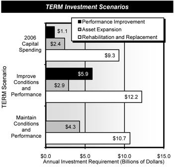
Since 1997, the C&P report has included a consistent set of TERM investment scenarios that assess the level of investment required to attain specific asset conditions and performance targets. The levels of investment required to attain these targets have been combined to construct a range of investment scenarios. The Maintain Conditions and Performance scenario projects the level of investment to maintain current average asset conditions over the 20 year period and to maintain current vehicle occupancy levels as transit passenger travel increases. In looking at the Maintain Conditions and Performance scenario, with a benefit-cost ratio of 1.0, a total of $15.1 billion per year is required. The Improve Conditions and Performance scenario projects the level of investment to raise the average condition of each major transit asset type to at least a level of "good," reduce average vehicle occupancy rates, and increase average vehicle speeds. In this scenario, annual requirements for rehabilitation and replacement are projected to be $12.2 billion, with asset expansion and performance improvements estimated at $2.9 and $5.9 billion respectively to total an annual estimate of $21.1 billion.

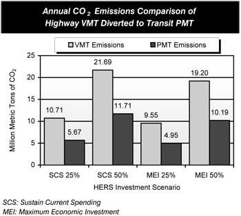
The variable rate user financing scenarios examined in the highway analysis assume a reduction in peak period VMT, a portion of which could be diverted to transit. The level of expansion investment required to support this increase in transit ridership while maintaining current transit performance at today's levels is examined. To do so, the analysis assumes that between 25 percent and 50 percent of diverted auto users shift to transit as their preferred modal choice, based on the projected VMT for the highway "Sustain Current Spending" (SCS) and "Maximum Economic Investment" (MEI) scenarios. Annual investment requirements modeled in TERM are significantly impacted by the increase in PMT on transit under all investment scenarios.

Chapter 9

Scenario Implications: Highways and Bridges

Chapter 9 provides supplemental discussion and analysis of key issues to assist in the interpretation of the selected capital investment scenarios presented in Chapter 8.

All of the investment/performance analyses in the C&P report are presented in constant 2006 dollars. It is difficult to predict inflation rates, and adjusting the constant dollar figures to nominal dollar values would add to the uncertainty of the overall results, particularly if inflation assumptions later proved incorrect. However, when applying these analytical findings in other contexts, such as comparing a particular scenario with nominal dollar revenue projections, it is sometimes necessary to adjust for inflation to ensure an accurate comparison.

Capital spending by all levels of government increased by 62.7 percent between 1997 and 2006, but did not keep pace with the 69.4 percent increase in the FHWA Composite Bid Price Index (BPI) over this period, due to a sharp increase in the cost of construction materials between 2004 and 2006.

The fixed rate financing version of the Sustain Conditions and Performance scenario implies that $40.0 billion per year of system expansion investment would be needed to achieve the scenario's goals; actual spending in 2006 by all levels of government for these types of improvements was only $30.0 billion. This finding is consistent with declines in operational performance noted in Chapter 4. The annual investment level identified for the system rehabilitation component of this scenario is $40.4 billion, which is close to the $43.5 billion of actual system rehabilitation spending in 2006. However, this gap is not evenly distributed across all types of roads and is wider for lower-ordered urban functional systems; this appears consistent with the decline in pavement conditions in recent years noted for these systems in Chapter 3.

The analyses in Chapters 7 and 8 assume gradual changes in investment at a fixed annual rate over time. Previous editions of the C&P had either assumed that investment would immediately jump to the average annual investment levels associated with each investment scenario or assumed that investment in any given year would be driven solely by benefit-cost ratio criteria. The latter approach frequently resulted in a significant front-loading of capital investment in the early years as the existing backlog of cost-beneficial improvements was addressed. The HERS model identifies $523.5 billion of cost-beneficial investments that could be made based on the current conditions and operational performance of the system, without regard to future travel growth; this is in addition to the $98.9 billion bridge backlog identified by NBIAS. If resources were available to immediately reduce the backlog in this fashion, HERS projects that there would be significant savings to users, even if annual investment later dropped off.

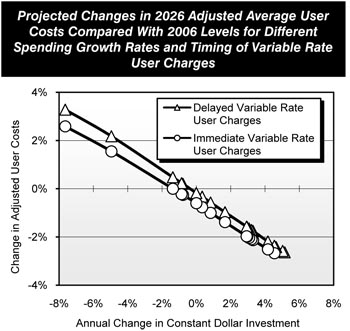
The variable rate financing analyses in Chapters 7 and 8 assume the immediate imposition of congestion pricing on a widespread basis. If the imposition of such charges were delayed by 10 years, HERS estimates that a higher level of investment would be needed to sustain adjusted annual average user costs, but that this could be achieved without increasing spending above the 2006 base year level in constant dollar terms. Regardless of the level of investment being analyzed, the projected average user costs associated with a delayed implementation of variable rate user charges would be higher than if such a financing mechanism were to be applied immediately.

Chapter 9

Scenario Implications: Transit

Chapter 9 considers a number of potential implications and limitations of the transit scenario analyses presented in Chapters 7 and 8. The intention is to provide a more comprehensive understanding of the assumptions used in scenario development as well as some alternative interpretations of the scenario results. Specifically, this section includes discussion of the following topics: ridership response to TERM investments; the potential impact of highway congestion pricing on CO2 emissions from both autos and transit vehicles; a comparison of PMT growth rates used by TERM's asset expansion module with the recent, actual PMT growth rates; and the potential impact of recent construction commodity price increases on transit investment costs.

Each of the three investment types considered by TERM—including the rehabilitation and replacement of existing assets, asset expansion, and performance improving investments—may draw varying levels of new transit ridership. First, the rehabilitation and replacement of aging transit assets results in improving the quality and reliability of transit services, improvements that are believed to attract new transit riders. At present, the responsiveness of ridership to changes in asset conditions is not well understood and, for this reason, these impacts are not currently modeled within TERM. Second, for TERM's annual asset expansion investments, given the weighted-average annual national growth rate of 1.5 percent, it is estimated that TERM's $4.7 billion investment in annual transit expansion (i.e., Maintain Performance) would support an additional 3.3 billion annual boardings by 2026, roughly 35 percent more than the current 9.5 billion annual boardings. Third, for the Improve Performance scenario, the estimate of $6.1 billion would generate 4.4 billion annual transit boardings by 2026, or 46 percent over current ridership levels.

Continuing with the presentation of congestion pricing in Chapter 8, Chapter 9 examines the impact that the portion of highway VMT that would shift away from peak period highway travel to transit alternatives in response to congestion pricing initiatives would have on CO2 emissions. This analysis indicates there is significant potential to reduce CO2 emissions by almost half for the assumed commuters diverting to transit from highways.

The "Transit Travel Growth" section describes how observed recent changes in PMT (historic growth rates) have diverged from the long-range demand forecasts used by TERM. The variance in PMT rates of change can be attributed to a variety of factors, including the strength of the U.S. economy, the prevalence of public transportation, and the price of gasoline. From 1997 to 2006, annual transit PMT increased from 39.2 billion to 49.5 billion, growing at an average annual rate of 2.6 percent.

Forecasting demand for public transportation services is an inexact science. TERM's projections of investments required to support the projected, natural growth in transit ridership are driven entirely by ridership and PMT forecasts provided by a sample of the nation's metropolitan planning organizations (MPOs). The average rate of PMT growth for 1991 to 2005 was 1.7 percent. The actual rate of increase for 2006 to mid-2008 well exceeds the forecast rate based on MPO projections of 1.5 percent on average for 2009 to 2026.

Pricing for materials and labor used in the construction industry have increased significantly in recent years, pushing the costs for constructing all types of capital projects upward. A discussion of construction material and labor inflation is also provided in Chapter 9.

Chapter 10

Sensitivity Analysis: Highways and Bridges

The usefulness of any investment scenario analysis depends on the validity of the underlying assumptions used to develop the analysis. Since there may be a range of appropriate values for several of the model parameters used in the HERS and NBIAS analyses presented in Chapter 7, this section explores the impacts of changing some of these assumptions pertaining to technology, travel growth, economic assumptions, the valuation of non-monetary benefits, and life span of bridges.

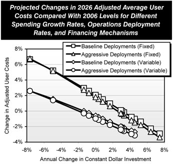
The baseline investment/performance analyses reflect the impacts of a continuation of existing trends in the deployment of operations strategies and intelligent transportation systems (ITS) technologies on highway performance. If a portion of the spending for system expansion in the baseline analyses were redirected to cover the capital and operating costs associated with a more aggressive rate of operations/ITS deployments, HERS projects that adjusted average user costs would be reduced for most of the investment levels analyzed. The baseline existing deployment trends assumption would result in superior performance outcomes only if total capital spending were to decrease significantly relative to 2006 levels. This analysis suggests that, if combined public and private investments were to be sustained at current levels or increased above those levels, serious consideration should be given to accelerating the rate of operations deployments.

Pavement technology can greatly extend the lifetime of a highway system. Assuming a one-third increase in typical pavement lives, HERS recommends directing a larger share of total funding to capacity expansion because pavement actions would not be needed as frequently. This would allow for improvements in both average pavement roughness and average traveler delay for most of the investment levels analyzed.

HERS assumes that the State-provided forecast for each sample highway segment represents the level of travel that will occur if a constant level of service is maintained on that facility. As noted in Chapter 4, however, the level of service has generally declined over time. Modifying the forecasts to match actual travel growth for the past 20 years would increase both overall congestion and the rate of pavement deterioration, both of which would cause the adjusted average highway user costs associated with any given level of capital investment to rise. Assuming fixed rate user financing, annual constant dollar spending would need to increase by between 6.41 percent and 7.45 percent to maintain average user costs in 2026 at base year 2006 levels, significantly higher than the 3.07 percent rate in the baseline analyses. Assuming variable rate user financing, spending would need to increase between 1.67 percent and 2.93 percent annually. Alternatively, if the trends that have caused travel growth per capita to rise over time were to cease and VMT were to grow only by the projected rate of increase in the total population, then current funding levels would be more than adequate to maintain adjusted user costs at base year levels.

The baseline investment/performance analyses are tied to the Energy Information Agency's reference case values for fuel prices; substituting in their high price forecast would result in lower projections for 2026 travel for all funding levels, regardless of the financing mechanism. This would lead to lower levels of average delay and average pavement roughness for any given funding level than were computed for the baseline analyses.

Chapter 10

Sensitivity Analysis: Transit

Chapter 10 examines the sensitivity of projected transit investment estimates by the Transit Economic Requirements Model (TERM) to variations in the values of exogenously determined model inputs including passenger miles traveled (PMT), capital costs, the value of time, and user travel cost elasticities.

TERM relies on forecasts of PMT in large urbanized areas to determine estimates of projected investment in the Nation's transit systems for the Maintain Performance scenario (i.e., current levels of passenger travel speeds and vehicle utilization rates) as ridership increases and the Improve Performance scenario (i.e., increase passenger travel speeds and reduce crowding).

PMT forecasts are generally made by metropolitan planning organizations (MPOs) in conjunction with projections of VMT. The average annual growth rate in PMT of 1.5 percent used in this report is a weighted average of the most recent MPO forecasts available. Transit investment estimates in the 2004 report were based on a projected PMT growth rate of 1.57 percent, from 92 of the Nation's largest metropolitan areas. PMT has increased at an average annual rate of 2.3 percent between 1997 and 2006 and by 3.1 percent between 2004 and 2006.

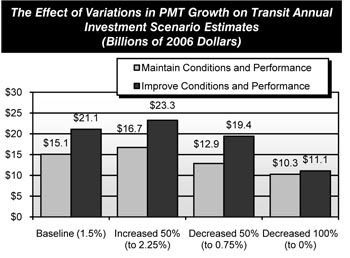
Varying the assumed rate of growth in PMT affects estimated transit investment both for the Maintain and Improve scenarios. A 50-percent change in growth will impact the cost to Maintain Conditions and Performance by an 11.0 percent increase or a 14.6 percent decrease, and the cost to Improve Conditions and Performance by a 10.2 percent increase or an 8.0 percent decrease. Investment estimated by both the Maintain and Improve scenarios would decrease significantly if PMT was assumed to remain constant.

Given the uncertainty of capital costs, a sensitivity analysis was performed to examine the effect of higher capital costs on the projected transit investment. A 25-percent increase in capital costs increases the investment estimated by the Maintain Conditions and Performance scenario by 9.9 percent and decreases the investment estimated by the Improve Conditions and Performance scenario by 20.7 percent. With this increase in costs, fewer investments are economically viable under this scenario compared with the Maintain Conditions and Performance scenario.

The value of time is used to determine the total benefits accruing to transit users from transit investments that reduce passenger travel time. Three scenarios were examined in relation to the base value of time of $11.20 per hour: (1) value of time is double, (2) value of time is half, and (3) value of time in constant 2006 dollars. Variations in the value of time were found to have a limited effect on the investment estimates because changes in the value of time have inverse effects on the demand for transit services. An increase in the value of time was found to reduce projected investment in modes with relatively slower transit services and to increase projected investment in modes with relatively faster transit services. The opposite occurs in response to a decrease in the value of time.

TERM considers user cost elasticities to estimate the changes in ridership, fare, and travel time costs resulting from infrastructure investment to increase speeds, decrease vehicle occupancy levels, and increase frequency. A doubling or halving of these elasticities was found to have a minimal effect (an increase of 0.4 percent and decrease of 6.5 percent, respectively) on projected investment.

Chapter 11

NHS Bridge Performance Projections

All bridges are important to the communities along the Nation's transportation system; however, the National Highway System (NHS) bridge network is extremely important because of the amount of traffic it carries.

Chapter 11 examines the impact of combining several bridge management strategies with different funding alternatives over a period of 50 years. The analyses presented in this chapter do not directly correspond to the 20-year capital investment scenarios referenced in other chapters.

Several metrics are considered: the bridge's average Sufficiency Rating (a composite measure taking into account factors such as a bridge's structural adequacy, functionality, and essentiality, on a scale of 0 to 100), the average Health Index (a measure of the structural integrity of individual bridge elements, on a scale of 0 to 100); and the percentage of NHS bridges with condition ratings of 5 or greater for deck, superstructure, and substructure (a measure of the general condition of major bridge components, on a scale of 0 to 9).

The Sufficiency Rating 50 strategy assumes that structures that reach a sufficiency rating of 50 or less are selected for replacement. The Age 50 strategy assumes that any structure that becomes 50 years or older during the analysis period will be replaced. The Health Index 75 strategy assumes that any structure with a health index equal to or less than 75 during the analysis period will be replaced. The Health Index 80 strategy assumes that any structure with a health index equal to or less than 80 during the analysis period will be replaced. The Health Index 85 strategy assumes that any structure with a health index equal to or less than 85 during the analysis period will be replaced.

An additional management strategy was included in the analysis to reflect selection of actions on bridges based on any action having a benefit-cost ratio of 1.0 or greater. This is the No Special Rules strategy.

Four funding alternatives were combined with one or all of the proposed management strategies – the Maximum Flat Funding alternative, the Maximum Ramped Funding alternative, the Unconstrained Funding alternative, and the Current Funding alternative.

The Maximum Flat Funding alternative provides funding at the maximum annual amount at which all allocated funds will be expended during the analysis period. The Maximum Ramped Funding alternative assumes an increase in spending at a fixed annual rate over 50 years. The Unconstrained Funding alternative assumes spending will be allocated on the management criteria in use and there is no limit to annual spending. The Current Funding alternative assumes funding will remain at the amount allocated for 2006. All amounts are in 2006 dollars.

In general, when comparing the various strategies, those that yield the higher values of the individual metrics both over the long term and the short term will provide a more desirable system.

The Sufficiency Rating 50 – Current Funding combination yielded the lowest values for all metrics except for substructure condition rating. The Age 50 – Maximum Flat Funding combination yielded the lowest substructure value in 2056. The remaining approaches provide much higher metric levels in 2056 and, depending on the minimum acceptable performance levels selected, yield a much higher performance level for the total NHS bridge network.

It is critical to understand the funding stream needed to implement any of the approaches. The ramped spending approach gradually increases investment, addressing an increasing number of needs each year. The flat spending approach may not provide enough funding to reduce the backlog. The No Special Rules approach projects a large influx of funding in 2007, followed by relatively flat funding.

Chapter 12

Transportation Serving Federal and Indian Lands

Federal and Indian lands have many uses. These include recreation, range and grazing, timber, minerals, watersheds, fish and wildlife, and wilderness. In recent years, recreational use has significantly increased, while resource extraction and cutting of timber have declined. These lands are also managed to protect their natural, scenic, scientific, and cultural value.

Roads on Indian lands provide access and mobility for residents and provide access to regional and national transportation systems. Tribal roads are essential for economic development and community development on reservations, providing critical access between housing and education, emergency centers, and places of employment.

Transportation plays a key role in the way people access and enjoy Federal lands. Approximately 329,000 miles of public roads are located on Federal lands, including 93,000 miles of State and local roads that provide access to and within these lands. Use of roads by private vehicles and tour buses continues to be the primary method of travel to and within Federal and Indian lands.

Although the Federal Highway Administration (FHWA) and its predecessors have worked to improve access to Federal lands for over a century, the Federal Lands Highway Program (FLHP) was only created in 1983. Today's FLHP is subdivided into four core areas: the Indian Reservation Roads, Park Roads and Parkways, Refuge Roads, and Public Lands Highway (Forest Highway and the Public Lands Highway Discretionary) Programs.

The primary purpose of the FLHP is to provide financial resources and technical assistance to support a coordinated program of public roads that service the transportation needs of Federal and Indian lands. The SAFETEA-LU authorizations for 2005 through 2009 for the FLHP total over $4.5 billion. During the past five fiscal years, the FLHP has improved, on average, about 1,000 miles of roads and 35 to 40 bridges per year.

The FHWA works with numerous Federal Land Management Agencies (FLMAs) while overseeing the FLHP. The four FLMAs that are most directly involved in the core areas of the FLHP are known as core partners; these include the U.S. Forest Service (USFS), the National Park Service (NPS), the Bureau of Indian Affairs (BIA), and the U.S. Fish and Wildlife Service (FWS).

The USFS estimates that, of the 29,200 miles of paved National Forest System Roads in 2006, approximately 39 percent were in good condition, compared with 29 percent in fair condition and 32 percent in poor condition. The NPS estimates that, of 5,450 miles of paved Park Roads and Parkways, approximately 11 percent were in good condition, while 48 percent were rated as fair and 41 percent were considered poor. The condition ratings estimated by the BIA for nearly 37,000 paved miles of Indian Reservation Roads are 16 percent good, 39 percent fair, and 45 percent poor. The FWS estimates that, of 415 miles of paved Refuge Roads, approximately 39 percent were in good condition, 32 percent were in fair condition, and 30 percent were in poor condition.

The FLHP supports the FLMAs beyond design and construction oversight by also providing funding and expertise for integrated transportation planning, road and bridge inspections, and other technical assistance activities. FLHP funds can be used for transportation planning, research, engineering, and construction of highways, roads, parkways, and transit facilities.

SAFETEA-LU established a $97 million Alternative Transportation in Parks and Public Lands Program. This program authorizes FTA grants for projects that improve mobility in parks and public lands. Eligible projects include the purchase of buses for new transit service, replacement of old buses and trams, construction of bicycle and pedestrian pathways, ferry dock replacement, intelligent transportation system components, and planning studies.

Chapter 13

Freight Transportation

The economy of the United States depends on freight transportation to link businesses with suppliers and markets. The transportation system in the United States moved an average of 53 million tons of freight worth $36 billion per day in 2002. Over the next three decades, the tonnage of goods to be moved is expected to increase by 2.0 percent each year, almost doubling between now and 2035.

Demands on the Transportation System

Most of the Nation's freight transportation infrastructure was developed before 1960. This older system moved goods from farm to market and from fort to port, and served industrial and population centers concentrated in the Northeast and the Midwest. Since 1960, however, population and manufacturing have grown in the South and on the West Coast, and international trade has changed the complexion of traditional corridors. Railroads and steamship companies accommodate enormous numbers of containers—a technological novelty five decades ago. Trucks serve new inland distribution centers beyond the urban fringe. Air carriers deliver parcels between any locations in the country over night.

The freight system must serve an economy that is increasingly decentralized and organized around just-in-time delivery. Much of this delivery is done by truck. The Interstate System carries half of truck travel and three-fourths of freight-hauling truck traffic that serves places at least 50 miles apart.

Freight and Congestion

As freight demand grows, it often creates congestion. Congested freight hubs include international gateways such as ports, airports, and border crossings, as well as domestic terminals and transfer points such as Chicago's rail yards. On the Nation's road network, the top 10 highway interchange bottlenecks cause an average of 1.5 million annual truck hours of delay each, compared to less than 250,000 annual hours of truck delay for other truck bottlenecks. Trucks are also a source of congestion when space and time for pickups and deliveries are limited. An estimated 947,000 hours of vehicle delay is attributable to delivery trucks parked curbside in dense urban areas.

Safety and Environmental Concerns

Freight transportation is not just an issue of throughput and congestion. Policymakers are increasingly focused on how freight transportation impacts air quality, and how hazardous materials can be safely moved. Policymakers are deliberating how to move the Nation's increasing volume of goods without compromising public safety and the quality of the environment.

The Economic Costs of Freight Transportation

Freight transportation has become cheaper over the past quarter century, contributing significantly to the Nation's economic productivity and growth. Several forces, however, are combining to increase costs in the years ahead. Congestion, higher fuel prices, and a shortage of labor in some sectors has increased the costs to carriers, and impacted the prices of goods. Over the three years ending in 2006, prices increased 13 percent for truck transportation, 27 percent for rail transportation, and 8 percent for scheduled air freight.

The Freight Challenge

SAFETEA-LU included several provisions designed to improve freight infrastructure. Among other provisions, SAFETEA-LU authorized $4.6 billion for certain freight-oriented investments, expanded eligibility under the Transportation Infrastructure Finance and Innovation Act (TIFIA) for freight projects, and modified the tax code to encourage investment through private activity bonds. Still, meeting the freight challenge is difficult due to the high cost of many improvements and the fact that much of the Nation's freight infrastructure is privately owned.

Chapter 14

Congestion Reduction Strategies

Congestion generally reflects a fundamental imbalance of supply and demand. Economists have long understood that such an imbalance stems from inefficient pricing, where the true costs of use are not reflected in the prices paid by users. This imbalance is also affected by the absolute volume of traffic (demand) on a given facility relative to its physical capacity (supply).

There are four broad ways to reduce congestion: add more capacity, use capacity more productively, reduce system demand, and create an efficient transportation market.

Strategic Addition of Capacity

Traditionally, transportation officials have dealt with congestion by expanding the capacity of the road network. Today, however, concerns about air pollution, noise, and urban sprawl often stand in the way of capacity additions. Equally significant, adding new capacity can be enormously expensive and physically challenging. Despite these challenges, major projects that reduce bottlenecks, add lanes, or modify traffic patterns can often provide system performance benefits that outweigh these costs.

System Operations and Management

Another approach is to use the transportation system more productively. Transportation officials can increase productivity by maximizing system performance in the first place and being prepared to recover as quickly as possible when disruptions occur.

Several tools are greatly improving system operations and management. Real-time traveler information allows travelers to decide how they will (or will not) use the transportation system. Traffic incident management is a planned and coordinated process to detect, respond to, and remove traffic incidents and restore capacity as safely and quickly as possible.

Work zones are second only to incidents as a source of delay from temporary capacity loss, and more effective management can minimize disruptions to the traveling public. Better monitoring of weather conditions and improved traffic signal timing and coordination can also enhance the productivity of the highway network.

Providing Better Transportation Choices

Another effective way to reduce the level of demand for using highways is to ensure that travelers have a variety of high-quality alternatives to choose from that meet their transportation needs. Travel Demand Management (TDM) increases the use of travel alternatives; spreads the timing of travel to less-congested periods; reduces the need for travel; and shifts the routing of vehicles to less-congested facilities. A more robust public transportation system, high-occupancy vehicle lanes, better bicycling and pedestrian facilities, flexible work schedules, and telecommuting are a few of the other alternatives to traditional highway transportation.

Road Pricing

Although the building of new facilities and better management and operation of roads are effective strategies in relieving congestion, they do not address one of its root causes: that most travelers do not pay the full cost of receiving transportation services. Congestion pricing—charging a price that will bring supply and demand into balance—relies on market forces and recognizes that trip values vary by individual.

Congestion pricing can take many forms. At the present time, variable pricing is typically applied on a limited access facility, such as a bridge, or in a congestion charging zone around a central business district. In the future, charging systems that use special technology may make it feasible to efficiently price entire road networks. Congestion pricing may also be applied to parking, encouraging travelers to alter their travel habits during peak periods.

Chapter 15

National Household Travel Survey

Since 1969, the National Household Travel Survey (NHTS) and related studies have provided key information on how the American public uses the Nation's highway system. The NHTS provides detailed data on the characteristics of travelers, trips, and vehicles. Data collection for the 2008 survey is currently underway. This Chapter includes selected findings from the 2001 survey.

Long-Distance Travel

Overall, about 2.6 billion long distance trips are taken by U.S. residents every year. These are trips of 50 miles or more away from home; in any given year, 169 million people (61 percent of the population) do not make any trips of this length. Business trips comprise nearly 30 percent of the long distance trips. Another 25 percent of trips involve visiting friends and relatives, while leisure trips, sight-seeing, and vacations make up another 25 percent.

Older Drivers

Americans aged 65 and older represent the fastest-growing segment of the U.S. population. The total mileage driven by these older Americans is projected to increase by 50 percent by 2020 and more than double by 2040. While older drivers tend to drive far fewer miles than younger drivers, they are more vulnerable to severe injuries. Per mile driven, elderly drivers (those over 80 years old) are more likely to die in a crash than any other age group.

Rising Fuel Cost

Almost 70 percent of all petroleum used in the United States goes for transportation. Recent increases in fuel costs have raised questions about the impact of higher fuel prices on driver behavior. In 2001, the average household spent $1,461 a year on motor fuel; by 2006, this cost had risen to an estimated $3,261. Despite higher fuel prices, passenger travel has continued to grow. This is due to population growth; the increased purchasing power of American households; and the continued dispersion of housing, workplace, and recreational locations.

Travel Characteristics of New Immigrants

For the first time since the early 1900s, immigrants comprise more than 10 percent of the American population, a total of 32 million people. Immigrants will provide a larger share of the labor force in the future, requiring agencies to rethink transportation options. Immigrants are five times more likely to take transit to work than native-born Americans. There is also a high use of carpools by Hispanic commuters, especially men.

Commuting

One in 12 American workers spent an hour or more commuting each way per day in 2001, up from one in 20 in 1995. The number of hour-long commutes has skyrocketed not only because workers are taking jobs farther from home, but because the same commutes are taking longer. More than one-quarter of workers with commutes of one hour or longer leave before 6 a.m. for their trip to work.

Travel Time and Congestion

Commuting is a major factor in metropolitan congestion. According to the 2001 NHTS, two-thirds of all commuters usually leave for work between 6:00 and 9:00 a.m., and more than 88 percent of these workers travel in private vehicles.

A significant number of non-work vehicle trips, however, are made during peak periods. From 1990 to 2001, morning peak period non-work trips on Mondays through Thursdays increased by 100 percent. Shopping trips (including those for the purpose of getting a meal) adds 31 billion VMT to morning peak volumes.

Travel to School

The percentage of children ages 6 to 12 driven to school in a private vehicle rose from 15 percent in 1969 to 50 percent in 2001. This change in travel behavior has led many transportation professionals to consider policies and programs that encourage walking and biking to school, especially for grade school children.