

Executive Summary
PART I
Description of Current System
The U.S. Department of Transportation's (DOT's) Transportation for a New Generation, a Strategic Plan for Fiscal Years 2014—18 presents five strategic goals:
- Safety — Improve public health and safety by reducing transportation-related fatalities, injuries, and crashes.
- State of Good Repair — Ensure that the United States proactively maintains critical transportation infrastructure in a state of good repair.
- Economic Competitiveness — Promote transportation policies and investments that bring lasting and equitable economic benefits to the Nation and its citizens.
- Quality of Life in Communities — Foster quality of life in communities by integrating transportation policies, plans, and investments with coordinated housing and economic development policies to increase transportation choices and access to transportation services for all.
- Environmental Sustainability — Advance environmentally sustainable policies and investments that reduce carbon and other harmful emissions from transportation sources.
Part I Structure
Chapter 1 outlines the trends in travel behavior of households and businesses and describes the freight transportation system. Chapter 2 describes the extent and use of highways, bridges, and transit systems. Chapter 3 addresses issues relating to the State of Good Repair Goal, while Chapter 4 relates to the Safety Goal. Chapter 5 covers topics relating to the Economic Competitiveness Goal, the Quality of Life in Communities Goal, and the Environmental Sustainability Goal. Chapter 6 provides data on highway and transit finance.
Transportation Performance Management
A recurring theme in Part I of this C&P report is the coming impact of changes under the Moving Ahead for Progress in the 21st Century Act (MAP-21). The cornerstone of the MAP-21 program transformation is the transition to a performance and outcome-based program. Performance measures will be established through a set of rulemakings; grant recipients will set performance targets based on these measures, and will periodically report on their progress toward meeting these targets. FHWA is implementing the MAP-21 requirements through six interrelated rulemakings:
- Statewide and Metropolitan/Nonmetropolitan Planning Rule
- Safety Performance Measures Rule (PM-1)
- Highway Safety Improvement Program (HSIP) Rule
- Pavement and Bridge Performance Measures Rule (PM-2)
- Asset Management Plan Rule
- System Performance Measures Rule (PM-3) (includes measures for freight movement and the Congestion Mitigation and Air Quality program).
CHAPTER 1
Personal Travel
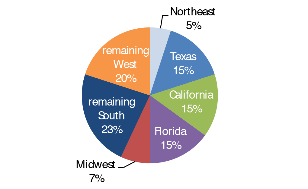
The Nation is becoming more populated, more diverse, and more urban. Three states (Texas, Florida, and California) are projected to account for nearly half of all national population growth through 2030, with the remainder concentrated in other States in the South and West (Census, 2010).
Overall, migration in the United States has slowed over the past few years, but the southern region showed gains from 2005 to 2010. New immigrants are especially likely to settle in California, New York, Texas, Florida, Illinois, and New Jersey.
Regional Migration and Growth
Expanding metropolitan areas, or "megaregions," have also spawned a network of metropolitan centers. Experts believe 75 percent of the U.S. population will reside in megaregions by 2050. The 11 emerging megaregions are the Northeast, Florida, Piedmont Atlantic, Gulf Coast, Great Lakes, Texas Triangle, Arizona Sun Corridor, Front Range, Cascadia, Northern California, and Southern California. Both freight travel and passenger travel are expected to increase within the megaregions, putting further demands on the transportation system.
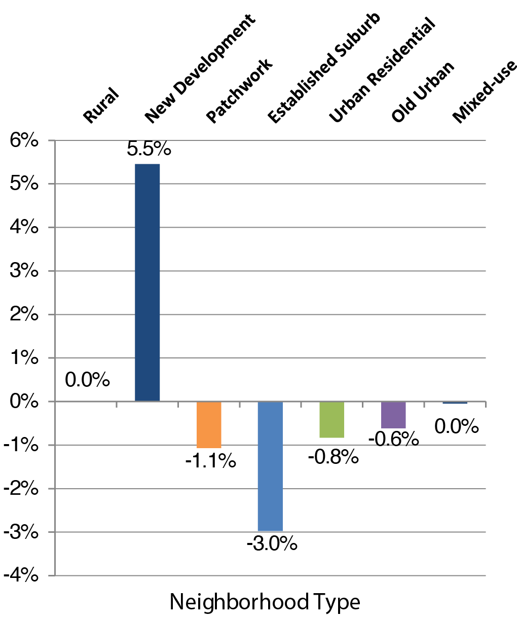
Young adults (20—34 years old) are gravitating to new suburban development near the fringes of metropolitan areas. In contrast, the share of young adults living in established suburbs declined in recent years.
Percentage Point Change in Young Adult Population (Ages 20—34 Years) by Neighborhood Type, 2000—2010
Low-income families are moving from city centers to suburban locations. In 1970, suburbs housed 25 percent of the poor; by 2010 the proportion was 33 percent .
CHAPTER 1
Freight Movement
Freight transportation is vital to the U.S. economy and the day-to-day needs of citizens. This sector has gained increasing attention under both MAP21 and the Fixing America's Surface Transportation Act (FAST Act). The success of freight planning across the United States, however, faces significant and varied challenges.
Current freight demands are straining existing system capacity, while freight movement across the United States is expected to increase. In 2012, the U.S. transportation system handled a record amount of freight: 54 million tons of product valued at $48 billion was shipped daily to 118.7 million U.S. households, 7.4 million business establishments, and 89,004 government institutions.
Freight transport and passenger transport are very different. Freight travel patterns tend to change more rapidly than passenger travel patterns in response to short-term economic fluctuations. Improvements targeted at general passenger travel are less likely to aid the flow of freight than are improvements targeted at freight demand.
Trucks transport most U.S. freight, accounting for 67.0 percent of freight tonnage and 64.1 percent of freight value in 2012. Trucking handles most of the lower-valued bulk tonnage, which includes agricultural products, local gasoline delivery, and municipal solid waste pickup, but is also critical for moving high value freight coming off of air cargo or other modes. Trucks are usually the main mode for freight trips of less than 500 miles. As gas prices fluctuate, this threshold will vary.
Virtually all carriers and freight facilities (such as railroad lines and some port terminals) are privately owned but use public highways and airways. This mix of ownership requires complex coordination by a variety of private and public stakeholders. The private sector owns $1.173 trillion in transportation equipment and $739 billion in transportation infrastructure, while the public sector maintains $686 billion in transportation equipment and $3.343 trillion in highway infrastructure.
Although most goods move short distances, usually less than 250 miles, freight often moves over multiple jurisdictions. As half the weight and two-thirds the value of freight products cross State or international boundaries, the benefits of this freight transportation might not accrue to the communities through which it travels. Both the interregional nature of many freight movements and the varying levels of support or opposition in local jurisdictions for freight-generating development can complicate the freight planning process. Assessing and measuring the impacts of full freight trips across multiple jurisdictions is often challenging for State and local transportation planners.
Freight transport-which accounted for 25.5 percent of all gasoline, diesel, and other fuels consumed by motor vehicles in 2013-can create safety and congestion challenges. Hazardous material transport is dangerous; hazardous material incidents across all modes totaled 15,433 in 2012. Increasing freight levels are adding to congestion in urban areas and on intercity routes.
CHAPTER 2
System Characteristics: Highways
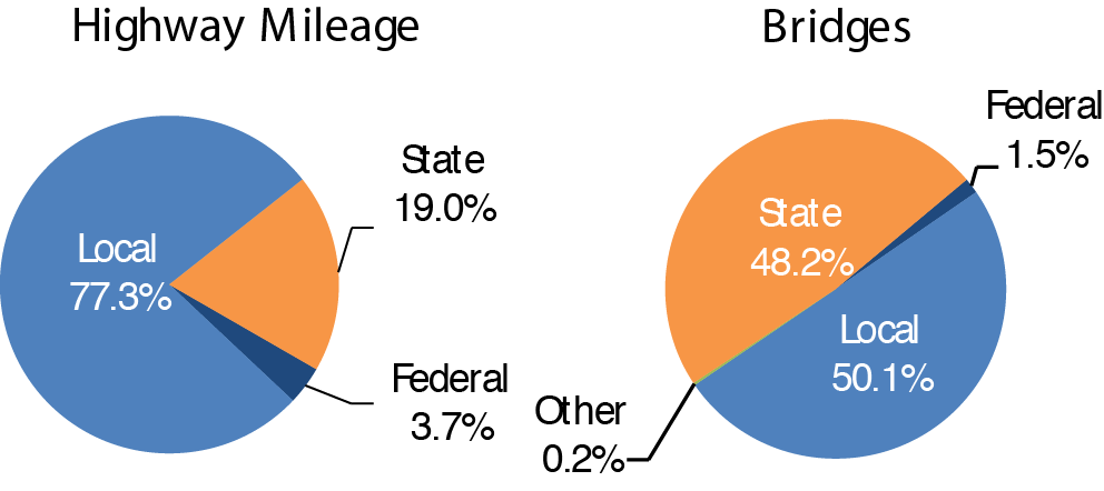
Although the Federal government provides significant financial support for the Nation's highways and bridges, it owns relatively few of these facilities. In 2012, State and local governments owned 96.3 percent of the Nation's 4,103,418 public road miles and 98.3 percent of the Nation's 607,380 bridges. These roads and bridges carried more than 2.9 trillion VMT.
Highway and Bridge Ownership by Level of Government
The Nation's roadway system is a vast network connecting places and people within and across national borders. The network facilitates movement of vehicles serving everything from long-distance freight needs to neighborhood travel. To accommodate the Nation's diverse travel needs, different types of roads are constructed to serve two primary purposes: access and mobility.
Roads are categorized into functional classifications to establish their purpose and to determine whether they are eligible for Federal-aid highway funding assistance. In general, public roads that are functionally classified higher than rural minor collector, rural local, or urban local are eligible for Federal-aid highway funding.
Nearly 73 percent of the public road mileage is located in rural settings with populations less than 5,000. Although only 27.1 percent of the public road mileage is located in urban areas with populations of 5,000 or more, the densely populated areas contribute 67.2 percent of VMT.
Similar to the breakdown of public road mileage, 73.6 percent of the Nation's bridges are in rural areas, while 26.4 are in urban areas.
| Percentages of Highway Miles, Vehicle Miles Traveled, and Bridges by Functional System, 2012 | |||
|---|---|---|---|
| Functional System | Highway Miles | Highway VMT | Bridges |
| Rural Areas (4,999 or less in population) | |||
| Interstate | 0.7% | 8.2% | 4.1% |
| Other Freeway and Expressway1 | 0.1% | 0.7% | |
| Other Principal Arterial1 | 2.2% | 6.8% | |
| Other Principal Arterial1 | 6.0% | ||
| Minor Arterial | 3.3% | 5.0% | 6.4% |
| Major Collector | 10.3% | 5.9% | 15.3% |
| Minor Collector | 6.4% | 1.8% | 7.9% |
| Local | 49.9% | 4.4% | 33.8% |
| Subtotal Rural Areas | 72.9% | 32.8% | 73.6% |
| Urban Areas (5,000 or more in population) | |||
| Interstate | 0.5% | 16.5% | 5.1% |
| Other Freeway and Expressway | 0.2% | 7.5% | 3.3% |
| Other Principal Arterial | 1.6% | 15.4% | 4.6% |
| Minor Arterial | 2.6% | 12.5% | 4.7% |
| Collector1 | 3.4% | ||
| Major Collector1 | 2.8% | 5.9% | |
| Minor Collector1 | 0.0% | 0.1% | |
| Local | 19.4% | 9.3% | 5.4% |
| Subtotal Urban Areas | 27.1% | 67.2% | 26.4% |
| Total | 100.0% | 100.0% | 100.0% |
| 1 Less functional system detail is available for bridges than for highways. Bridges on rural Other Freeway and Expressway are included under the rural Other Principal Arterial category. Bridges on urban Major Collector and urban Minor Collector are combined into a single urban Collector category. | |||
CHAPTER 2
System Characteristics: Transit
Most transit systems in the United States report to the National Transit Database (NTD). In 2012, 822 systems served 497 urbanized areas, which have populations greater than 50,000. In rural areas, 1,637 systems were operating. Thus, the total number of transit systems reporting to NTD in 2012 was 2,264.
Modes. Transit is provided through 18 distinct modes in two major categories: rail and nonrail. Rail modes include heavy rail, light rail, streetcar, commuter rail, and other less common modes that run on fixed tracks. Nonrail modes include bus, commuter bus, bus rapid transit, demand response, vanpools, other less common rubber-tire modes, ferryboats, and aerial tramways. This edition of the C&P report includes four new modes: commuter bus and bus rapid transit (previously reported as fixed-route bus); hybrid rail, which shares characteristics of light rail and commuter rail; and demand-response taxi (previously reported as demand response).
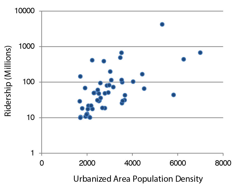
Urbanized Areas, Population Density, and Demand. Based on the 2010 census, the average population density of the United States is 82.4 people per square mile. The average population density of all 498 urbanized areas combined is 2,510 people per square mile. The average density for the 50 most-populated areas is 3,132 people per square mile. The chart shows the relationship between ridership and urbanized area density for the top 50 areas in 2012.
National Transit Assets
- Of the 162,830 vehicles in urban and rural areas, most are buses, cutaways (short buses), vans, and rail vehicles (passenger cars).
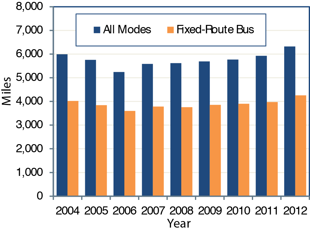
- Rail systems operate on 12,617 miles of track, and fixed-route bus systems operate over 252,800 route miles.
- Urban and rural areas have 3,281 stations and 1,720 maintenance facilities
2012 Urbanized Area Density vs. Ridership (Top 50 Areas in Population)
ADA Compliance. The Americans with Disabilities Act of 1990 (ADA) prohibits discrimination and ensures equal opportunity and access for persons with disabilities. The act requires transit agencies to provide accessible vehicles (e.g., with lifts) and stations with barriers on platforms, ramps, elevators and other elements. The level of ADA compliance is high for the national fleet, but lower for rail stations, particularly for old heavy rail systems built before the passing of the ADA.
CHAPTER 3
System Conditions: Highways
Pavement and bridge conditions directly affect vehicle operating costs because deteriorating pavement and bridge decks increase wear and tear on vehicles and repair costs. Poor pavement also can affect travel time costs if road conditions force drivers to reduce speed and can increase the frequency of crash rates. Poor bridge conditions can force trucks to detour to alternative routes, leading to increased travel time and delays and introducing increased freight impacts to other communities.
The Highway Performance Monitoring System (HPMS) collects data on pavement ride quality on Federal-aid highways. Between 2002 and 2012, the percentage of Federal-aid highway mileage classified as acceptable decreased from 87.4 percent to 80.3 percent . When weighted by VMT during the same period, however, acceptable ride quality decreased from 85.3 percent to 83.3 percent .
| Pavement Ride Quality on Federal-Aid Highways, 2002—2012 | |||||
|---|---|---|---|---|---|
| 2002 | 2008 | 2012 | |||
| By Mileage | |||||
| Acceptable (Good + Fair) | 87.4% | 84.2% | 80.3% | ||
| Poor | 12.6% | 15.8% | 19.7% | ||
| Weighted By VMT | |||||
| Acceptable (Good + Fair) | 85.3% | 85.4% | 83.3% | ||
| Poor | 14.7% | 14.6% | 16.7% | ||
Although States were instructed to collect pavement data differently in 2009, the variance between mileage and VMT data suggests that ride quality on less-traveled Federal-aid highways has significantly declined since 2002.
Bridges are a vital component of the Nation's highway system. One term used to classify bridges is "structurally deficient." Structural deficiencies are characterized by deteriorated conditions of primary bridge components and potentially reduced load carrying capacity and waterway adequacy, but do not imply safety concerns.
The National Bridge Inventory (NBI) includes data for bridge conditions. The total number of bridges reported in the NBI increased by 16,137 between 2002 and 2012, but the number of bridges classified as structurally deficient decreased by 17,282. During that time, the share of bridges classified as structurally deficient decreased from 14.2 percent to 11.0 percent .
| Structurally Deficient Bridges (Systemwide), 2002—2012 | |||
|---|---|---|---|
| 2002 | 2008 | 2012 | |
| Count | |||
| Total Bridges | 591,243 | 601,506 | 607,380 |
| Structurally Deficient | 84,031 | 72,883 | 66,749 |
| percent Structurally Deficient | |||
| By Bridge Count | 14.2% | 12.1% | 11.0% |
| Weighted by Deck Area | 10.4% | 9.3% | 8.2% |
| Weighted by Traffic | 8.0% | 7.2% | 5.9% |
As part of its ongoing efforts to encourage the integration of Transportation Performance Management principles into project selection decisions and to implement related provisions in MAP-21, FHWA has proposed moving to "Good" and "Poor" classifications to measure pavement and bridge conditions. Future C&P reports will integrate the final measures that emerge after a rulemaking process is completed.
CHAPTER 3
System Conditions: Transit
Transit asset infrastructure in the C&P report includes five major asset groups.
| Major Asset Categories | ||
|---|---|---|
| Asset Category | Components | |
| Guideway Elements | Tracks, ties, switches, ballasts, tunnels, elevated structures, bus guideways | |
| Maintenance Facilities | Bus and rail maintenance buildings, bus and rail maintenance equipment, storage yards | |
| Stations | Rail and bus stations, platforms, walkaways, shelters | |
| Systems | Train control, electrification, communications, revenue collection, utilities, electrification, signals and train stops, centralized vehicle/train control, substations | |
| Vehicles | Large buses, heavy rail, light rail, commuter rail passenger cars, nonrevenue vehicles, vehicle replacement parts | |
Condition Rating. FTA uses a capital investment needs tool, TERM, to measure the condition of transit assets. The model uses a numeric scale that ranges from 1 to 5.
| Definition of Transit Asset Conditions | ||
|---|---|---|
| Rating | Condition | Description |
| Excellent | 4.8—5.0 | No visible defects, near-new condition |
| Good | 4.0—4.7 | Some slight defective or deteriorated components |
| Adequate | 3.0—3.9 | Moderately defective or deteriorated components |
| Marginal | 2.0—2.9 | Defective or deteriorated components in need of replacement |
| Poor | 1.0—1.9 | Seriously damaged components in need of immediate repair |
The replacement value of the Nation's transit assets was $847.5 billion in 2012, 49 percent of which was guideway elements.
The relatively large proportion of guideway elements and systems assets that are rated below condition 2.0 (poor), and the magnitude of the $140-billion investment required to replace them represent major challenges to the rail transit industry.
| 2012 Asset Categories Rated Below Condition 2.0 (Poor) | |
|---|---|
| Asset Category | Percentage in Poor Condition |
| Guideway Elements | 31.4 |
| Systems | 15.1 |
| Facilities | 4.8 |
| Vehicles | 4.0 |
| Stations | 2.1 |
State of Good Repair (SGR). An asset is deemed in a state of good repair if its condition rating is 2.5 or higher. An agency mode is in SGR if all its assets are rated 2.5 or higher.
Trends in Urban Bus and Rail Transit Fleet not in SGR. The average condition rating for bus and rail fleets did not change much between 2002 and 2012, ranging between 3.0 and 3.3 for buses, and remaining constant for rail at 3.5. The percentage of the bus fleet not in SGR also did not change much, ranging between 10 and 12 percent . For rail, the percentage decreased from 4.6 to 2.8 percent .
| 2012 Transit Assets not in SGR (percent) | |||
|---|---|---|---|
| Category | Bus | Rail | All |
| Guideway Elements | 5.5 | 35.1 | 34.6 |
| Systems | 17.2 | 17.1 | 17.1 |
| Stations | 11.5 | 37.8 | 37.5 |
| Facilities | 7.4 | 24.3 | 15.3 |
| Vehicles | 9.8 | 2.8 | 7.2 |
CHAPTER 4
Safety: Highways
In 2012, 31,006 fatal crashes took place on roads in the United States; in the same year, approximately 1.63 million nonfatal injury crashes and 3.95 million property damage-only crashes occurred.
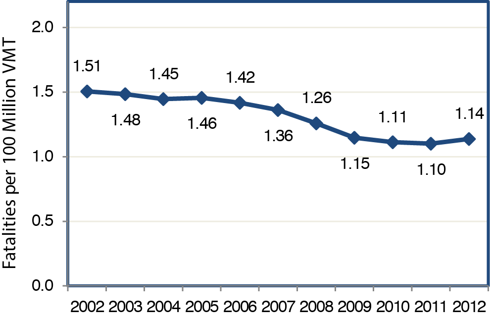
The number of fatalities related to the operation of motor vehicles dropped by 21.4 percent from 2002 to 2012, from 43,005 to 33,782. Over the same period, the fatality rate per 100 million VMT dropped from 1.51 to 1.14. Relative to recent years, the number of fatalities in 2012 was up from a low of 32,479, while the fatality rate was up slightly from a low of 1.10, reached in 2011.
Annual Highway Fatality Rates, 2002—2012
The DOT strategic goal on safety is "Improve public health and safety by reducing transportation-related fatalities and injuries for all users, working toward no fatalities across all modes of travel." In support of this goal, FHWA oversees the Highway Safety Improvement Program (HSIP), which requires a data-driven, strategic approach to improving highway safety on all public roads that focuses on performance. Use of HSIP funds is driven by a Strategic Highway Safety Plan (SHSP), which each State develops in cooperation with a broad range of multidisciplinary stakeholders.
When it occurs, a crash is generally the result of numerous contributing factors. Roadway, vehicle, driver, passenger, and nonoccupant factors all have an impact on the safety of the Nation's highway system. FHWA focuses on infrastructure design and operation to address roadway factors. Based on analyses of crash data, FHWA has established three focus areas: roadway departures, intersections, and pedestrian crashes. In 2012, roadway departure, intersection, and pedestrian fatalities accounted for 52.2 percent , 21.7 percent , and 14.1 percent , respectively, of all crash fatalities. That these three categories overlap one another should be noted, such as when a roadway departure crash results in a pedestrian fatality.
| Highway Fatalities by Crash Type, 2002—2012 | |||
|---|---|---|---|
| Crash Type | 2002 | 2012 | percent Change |
| Roadway Departure-Related | 25,415 | 17,532 | -31.0% |
| Intersection-Related | 9,273 | 7,279 | -21.5% |
| Pedestrian-Related | 4,851 | 4,743 | -2.2% |
Although progress has been made from 2002 to 2012 in reducing these types of fatalities, pedestrian fatalities have increased since 2009. Nonmotorist fatalities (including pedestrians, bicyclists, etc.) increased to 5,692 in 2012, up from 5,630 in 2002 and 4,888 in 2009.
CHAPTER 4
Safety: Transit
Rates of injuries and fatalities on public transportation generally are lower than for other modes of transportation. Nonetheless, serious incidents do occur, and the potential for catastrophic events remains. Several transit agencies have had major accidents in recent years. The National Transportation Safety Board has investigated several of these accidents and has issued reports identifying the factors that contributed to them. Since 2004, the National Transportation Safety Board has reported on 9 transit accidents that, collectively, resulted in 15 fatalities, 297 injuries, and more than $30 million in property damage.
Most injuries and fatalities in transit result from collisions, and most victims are not passenger or patrons. They are pedestrians, automobile drivers, bicyclists, or trespassers. Patrons are individuals in stations who are waiting to board or just got off transit vehicles. In 2012, of the 265 fatalities, only 4 percent were passengers. In 2002, of the 175 fatalities, the share of passenger fatalities was similarly small, 6 percent . The most striking change over that time has been the increase in the percentage of suicides, from 8 percent in 2002 to 23 percent in 2012.
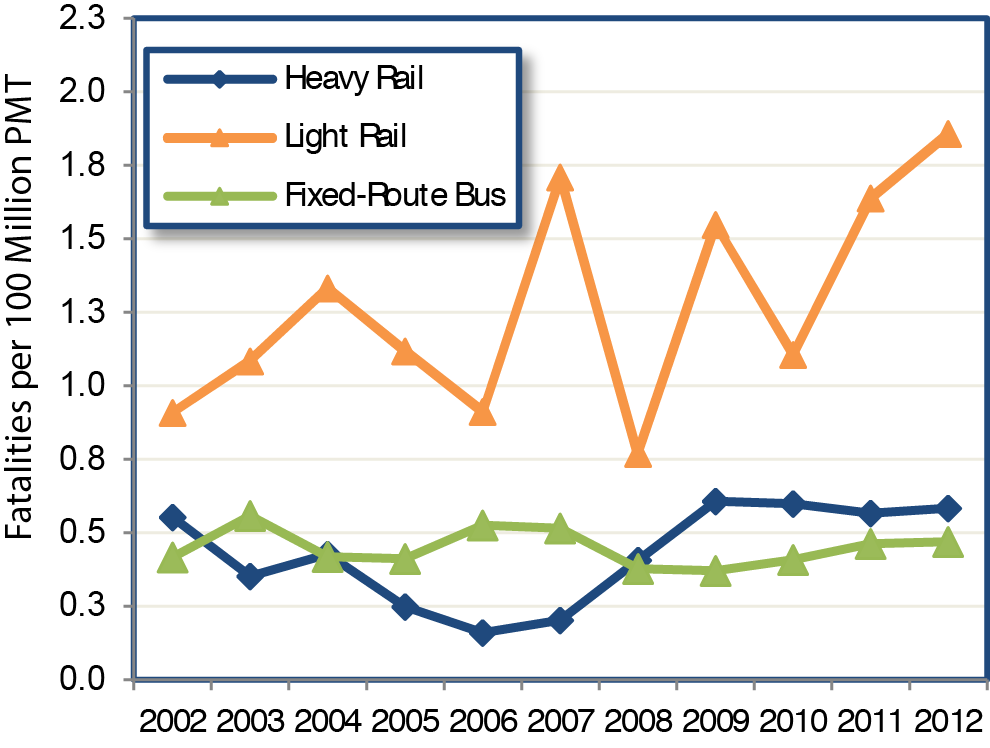
The Federal Transit Administration reports the rate of fatalities per 100 million passenger miles traveled. This rate did not change significantly between 2002 and 2012 for bus and heavy rail, the two largest modes and the ones with the most fatalities. The rate for light rail, which includes streetcars, is more volatile and has increased over the past 10 years due to a significant increase in service and number of systems.
Fatalities by Type of Person, 2012 and 2002
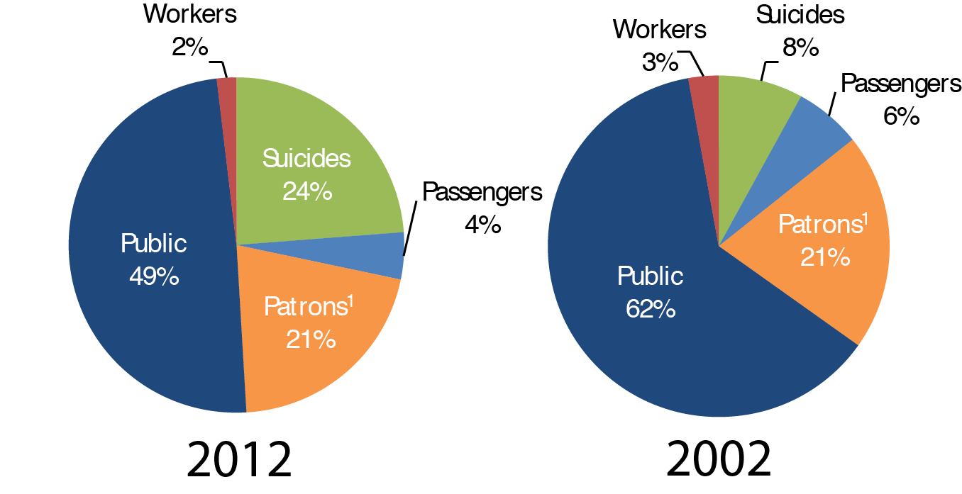
1Includes individuals waiting for or leaving transit at stations; in mezzanines; on stairs, escalators, or elevators; in parking lots; or at other transit-controlled property.
Annual Transit Fatality Rates per 100 Million Passenger Miles Traveled for Fixed-Route Bus, Heavy Rail, and Light Rail,
2002—2012
CHAPTER 5
System Performance: Highways
This chapter relates to three goals presented in DOT's FY 2014—18 Strategic Plan: (1) Economic Competitiveness, (2) Quality of Life in Communities, and (3) Environmental Sustainability.
Economic Competiveness: Congestion harms the U.S. economy and wastes time, fuel, and money. The Texas Transportation Institute's Urban Mobility Scorecard estimates that in 2012, on average, each commuter was delayed 41 hours due to congestion. Congestion wastes 6.7 billion hours and 3 billion gallons of fuel for the Nation as a whole, at a total cost of $154.2 billion in 2012.
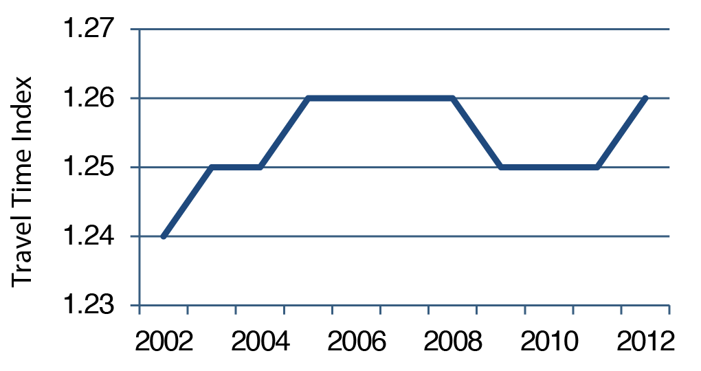
The Travel Time Index is calculated as the ratio of travel time required to make a trip during the congested peak period to travel time for the same trip during the off-peak period in noncongested conditions. Based on this measure, congestion rose from 2002 to 2008 before dropping briefly during the recent recession; by 2012, it had risen close to the levels observed before the recession.
Travel Time Index for Urbanized Areas, 2002—2012
Congestion can be recurring or nonrecurring; most travelers are less tolerant of unexpected delays than they are of everyday congestion. One relatively new source of data for measuring congestion and reliability is the National Performance Management Research Data Set (NPMRDS), which supports the Freight Performance Measures and Urban Congestion Report programs. FHWA measures freight highway congestion using truck probe data from global positioning system equipment. Truck probe data in the NPMRDS also measure corridor-level travel time reliability.
Quality of Life: Fostering livable communities is a continued goal of DOT. Progress is being made on measuring the impact of investments on increasing transportation choices and access to transportation services. Relevant tools such as the Location Affordability Portal, Sustainable Communities Indicator Catalog, Infrastructure Voluntary Evaluation Sustainability Tool, and Community Vision Metrics Web Tool are being used to support quality of life goals in communities.
Environmental Sustainability: Preparing for climate change is critical for protecting the integrity of the transportation system. One-fourth of the greenhouse gas emissions causing climate change in the United States is derived from the transportation sector. FHWA is partnering with State DOTs, MPOs, and Federal Land Management Agencies to develop strategies to reduce greenhouse gas emissions from transportation sources and build climate resilient transportation systems.
CHAPTER 5
System Performance: Transit
The transit industry has largely succeeded in meeting the demand for its services in communities across the country. Transit data from the end of the past decade show steady increases in service provided and consumed, commensurate with the growth of the urbanized population.
Between 2002 and 2012, the geographic coverage of transit significantly increased. New and extended commuter modes such as vanpools and commuter rail have reached areas previously accessible only by automobile. Light rail systems served 33 communities in 2012, compared with 22 in 2000. This light rail growth has increased the number of revenue service hours by 15 percent , the number of unlinked trips by 14 percent , and the number of passenger miles by 20 percent . The relatively larger increase in passenger miles is due to longer average trip lengths, which could be due to an expansion of service to outlying suburbs.
In 2004—2012, maintenance performance improved (vehicle revenue miles between mechanical failures). Over these 6 years, the average number of miles between failures increased by 21 percent .
Mean Distance Between Failures, Directly Operated Service, 2004—2012
Transit ridership is greatly affected by employment. Transit ridership increased significantly from July 2006 to January 2009 and then plummeted following the 2009 economic crisis. Relatively low fuel prices and employment levels characterized this crisis. Employment, fuel prices, and ridership all increased from 2010 to 2012.
Transit Ridership versus Employment, 2006—2012
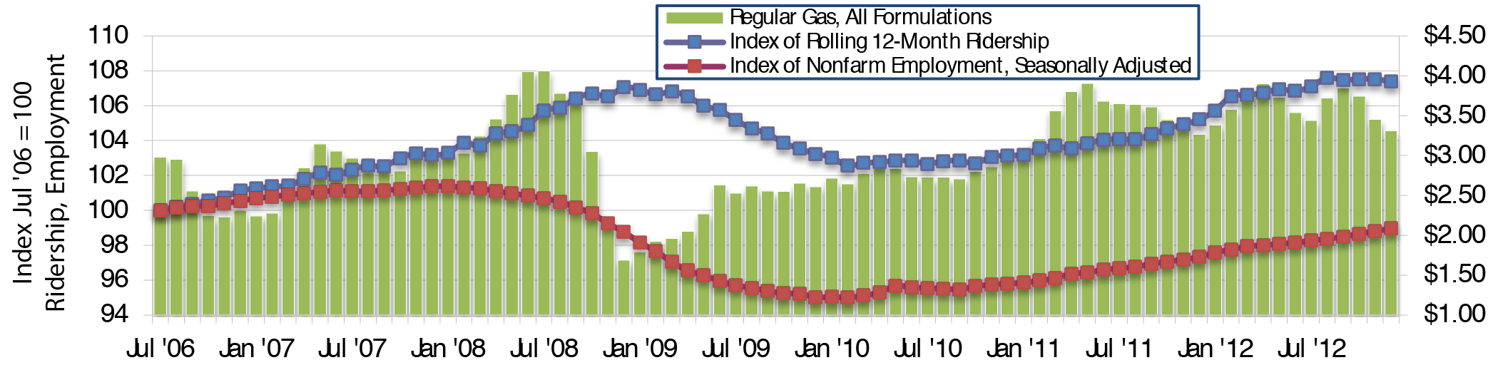
Sources: National Transit Database, U.S. Energy Information Administration's Gas Pump Data History, and Bureau of Labor Statistics' Employment Data.
CHAPTER 6
Finance: Highways
Combined expenditures for highways by all levels of government totaled $221.3 billion in 2012, with the Federal government funding $47.4 billion [including $3.0 billion authorized by the American Recovery and Reinvestment Act of 2009 (Recovery Act)], States $105.8 billion, and local governments $68.1 billion. Most of the Federal funding was in the form of grants to State and local governments; direct Federal expenditures for federally owned roads, highway research, and program administration totaled $3.2 billion.
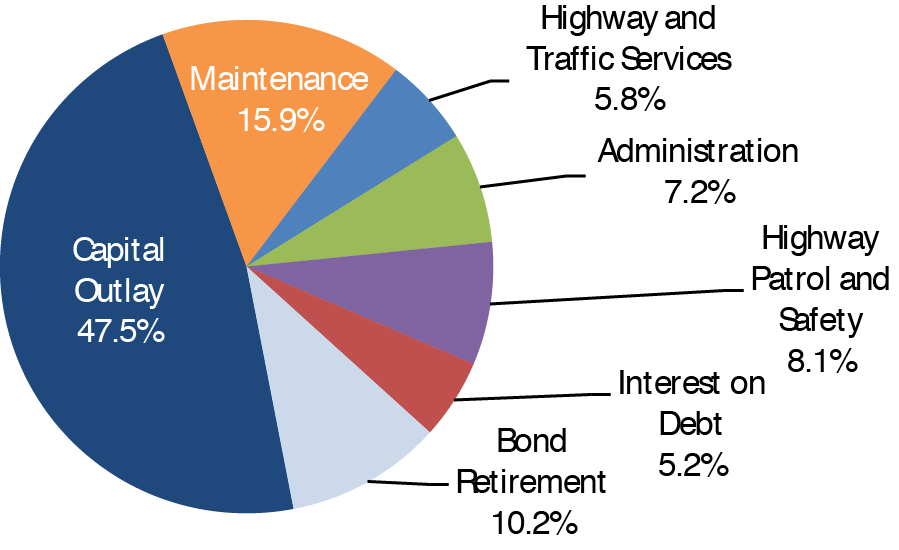
Highway capital spending totaled $105.2 billion, or 47.5 percent of total highway spending in 2012. Spending on maintenance totaled $35.1 billion, $12.9 billion was for highway and traffic services, $16 billion was for administrative costs (including planning and research), $17.8 billion was spent on highway patrol and safety, $11.6 billion was for interest on debt, and $22.6 billion was used to retire debt.
Highway Expenditure by Type, 2012
Total highway spending increased 62.8 percent from 2002 to 2012, averaging 5.0 percent per year. (In inflation-adjusted constant-dollar terms, highway spending grew by 2.6 percent per year). Expenditures funded by local governments grew by 7.2 percent per year, outpacing annual increases at the State and Federal levels of 4.4 percent and 3.7 percent , respectively. Over this period, the share of total highway expenditures funded by the Federal government dropped from 24.1 percent to 21.4 percent , while the federally funded share of highway capital spending dropped from 46.1 percent to 43.1 percent .
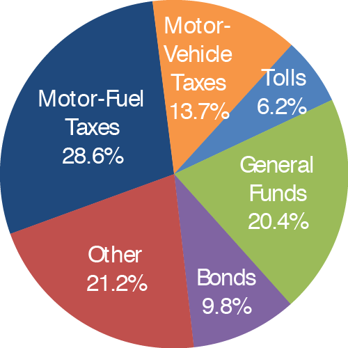
Combined revenues generated for use on highways by all levels of government totaled $216.6 billion in 2012 (the difference between expenditures and receipts is the amount drawn from reserves). In 2012, $105.2 billion (48.6 percent ) of total highway revenues came from highway user charges-including motor-fuel taxes, motor-vehicle fees, and tolls. Other major sources for highways included general fund appropriations of $44.1 billion (20.4 percent ) and bond proceeds of $21.3 billion (9.8 percent ). All other sources, such as property taxes, other taxes and fees, investment income, and other receipts, totaled $46.0 billion (21.3 percent ).
Revenue Sources for Highways, 2012
CHAPTER 6
Finance: Transit
In 2012, $58.0 billion was generated from all sources to finance urban transit. Transit funding comes from public funds that Federal, State, and local governments allocate and system-generated revenues that transit agencies earn from the provision of transit services. Of the funds generated in 2012, 73.3 percent came from public sources and 26.7 percent came from system-generated funds (passenger fares and other system-generated revenue sources). The Federal share was $10.9 billion (25.5 percent of total public funding and 18.7 percent of all funding).
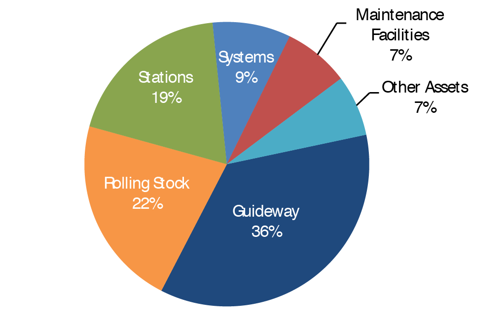
Guideway assets use the largest share of capital-36 percent ($6 billion)-for expansion and rehabilitation projects.
2012 Urban Capital Expenditure by Asset Category
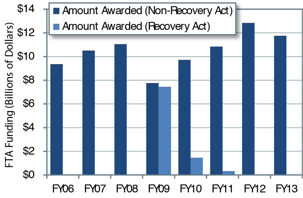
The American Recovery and Reinvestment Act of 2009 (Recovery Act) nearly doubled the total funding for urban transit.
Urban Recovery Act Funding Awards Compared to Other FTA Fund Awards
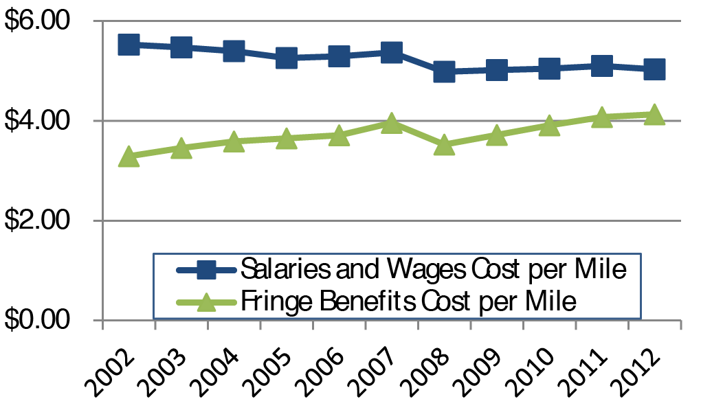
From 2002 to 2012, for the top 10 transit agencies, fringe benefits increased at the highest rate of any operating cost category on a per-mile basis. Over this period, fringe benefits increased at an annual compound average rate of 2.3 percent . Meanwhile, salaries and wages decreased by 1 percent .
Salaries and Wages and Fringe Benefits, Average Cost per Mile-Urbanized Areas Over 1 Million, 2002—2012 (Constant Dollars)
Part II
Investment/Performance Analysis
The methods and assumptions used to analyze future highway, bridge, and transit investment scenarios for this report are continuously evolving to incorporate new analytical methods, new data and evidence, and changes in transportation planning objectives. Estimates of future requirements for highway investment, as reported in the 1968 National Highway Needs Report to Congress, began as a combined "wish list" of State highway "needs." Over time, simulation models were developed that applied engineering standards to identify system deficiencies and the investments necessary to remedy these deficiencies. The current generation of analytical tools applied in this report each combine economic analysis with engineering principles in their identification of future capital investment needs.
The economic approach to transportation investment decision-making entails analyzing and comparing benefits and costs. Investments that yield benefits with values exceeding their costs increase societal welfare and are thus considered "economically efficient." To be reliable, such analyses must adequately consider the range of possible benefits and costs and the range of possible investment alternatives. A comprehensive benefit-cost analysis of a transportation investment would consider all potentially significant impacts on society and value them in monetary terms to the extent feasible. For some types of impacts, monetary valuation is facilitated by the existence of observable market prices; such prices are generally available for inputs to the costs of providing transportation infrastructure, such as prices for concrete to build highways or prices for new buses. For some other types of impacts for which market prices are not available, monetary values can be inferred from behavior or expressed preferences. In this category are savings in non-business travel time and reductions in the risk of crash-related fatalities or other injury. For still other impacts, monetary valuation might not be possible because of difficulties with reliably estimating the impact of the improvement, placing a monetary value on that impact, or both. Even when possible, reliable monetary valuation might require time and effort that would be out of proportion to the likely importance of the impact concerned and the inherent uncertainty in the estimates. Benefit-cost analyses of transportation investments therefore typically omit valuing certain impacts that nevertheless could be of interest.
The Highway Economic Requirements System (HERS), National Bridge Investment Analysis System (NBIAS), and Transit Economic Requirements System (TERM) used to develop the analyses presented in Chapters 7 through 10 each omit various types of investment impacts from their benefit-cost analyses. To some extent, such omissions reflect the national scope of their primary databases: Such broad geographic coverage requires some sacrifice of detail to stay within feasible budgets for data collection. The analyses do not consider, for example, environmental impacts of increased water runoff from highway pavements, barrier effects of highways on human and animal populations, and health benefits from the additional walking activity when travelers use transit rather than cars.
Although HERS, NBIAS, and TERM all use benefit-cost analysis, their methods for implementing this analysis differ significantly. These highway, bridge, and transit models each rely on separate databases, making use of the specific data available for each mode of the transportation system and addressing issues unique to that mode. The three models have not yet evolved to the point where direct multimodal analysis is possible; currently the models provide no direct way to analyze the impact that a given level of highway investment in a particular location would have on the transit investment in that vicinity (or vice versa).
Chapter 7 analyzes the projected impacts of alternative levels of future investment on measures of physical condition, operational performance, and benefits to system users. Each alternative pertains to investment from 2013 through 2032, which is presented as an annual average level of investment and as the annual rates of increase or decrease in investment that would produce that annual average. Both the level and rate of growth in investment are measured using constant 2012 dollars.
Chapter 8 examines several scenarios distilled from the investment alternatives considered in Chapter 7. Some of the scenarios are oriented around maintaining aspects of system condition and performance or achieving a specified minimum level of performance, while others link to broader measures of system user benefits. The scenarios included in this chapter are intended to be illustrative and do not represent comprehensive alternative transportation policies; the U.S. Department of Transportation (DOT) does not endorse any of these scenarios as a target level of investment.
Chapter 9 explores some of the implications of the scenarios presented in Chapter 8 and contains some additional policy-oriented analyses addressing issues not covered in Chapters 7 and 8. As part of this analysis, highway traffic projections from previous editions of the C&P report are compared with actual outcomes to elucidate the value and limitations of the projections presented in this edition. Chapter 9 also discusses the revised method for estimating transit travel growth rates introduced in this report.
The three investment analysis models used in this report are deterministic, not probabilistic: They provide a single projected value of total investment for a given scenario rather than a range of likely values. As a result, the element of uncertainty in these projections is amenable only to general characterizations based on the characteristics of the projection process; estimates of confidence intervals cannot be developed.
Chapter 10 presents sensitivity analyses that explore the impacts on scenario projections of varying some of the key assumptions. The investment scenario projections in this report are developed using models that evaluate current system condition and operational performance and make 20-year projections based on assumptions about future travel growth and a variety of engineering and economic variables. The accuracy of these projections depends, in large part, on the realism of these assumptions.
Because the future rate of growth in transit travel is uncertain, Chapter 7 considers alternative high and low values for this parameter. Chapter 10 likewise varies the assumed rate of growth in highway travel and the values assumed for the discount rate, the value of travel time savings, and other assumed parameters.
Chapter 7
Potential Capital Investment Impacts: Highways
NBIAS evaluates rehabilitation and replacement needs for all bridges. HERS evaluates needs associated with pavement resurfacing or reconstruction and widening needs, including those associated with bridges. HERS analyses are limited to Federal-aid highways, as HPMS does not collect data for other roads.
All levels of government combined spent $105.2 billion on highway capital outlay in 2012, including $16.4 billion for the types of bridge improvements modeled in NBIAS, and $57.4 billion on Federal-aid highways for the types of capital improvements modeled in HERS. The remaining $31.4 billion was divided about evenly between spending on non-Federal-aid highways on the same types of improvements that are modeled in HERS and on types of capital improvements covered by neither model.
The rate of future travel growth can significantly influence the projected future conditions and performance of the highway system. For the HERS and NBIAS analyses presented in this report, future travel volumes were tied to a 20-year national-level forecast averaging 1.04-percent growth per year. As this rate of growth was lower on average than the State projections reflected in HPMS and NBI, future traffic levels for individual highway sections and bridges were proportionally reduced so that the overall rate of growth would match the nationwide forecast.
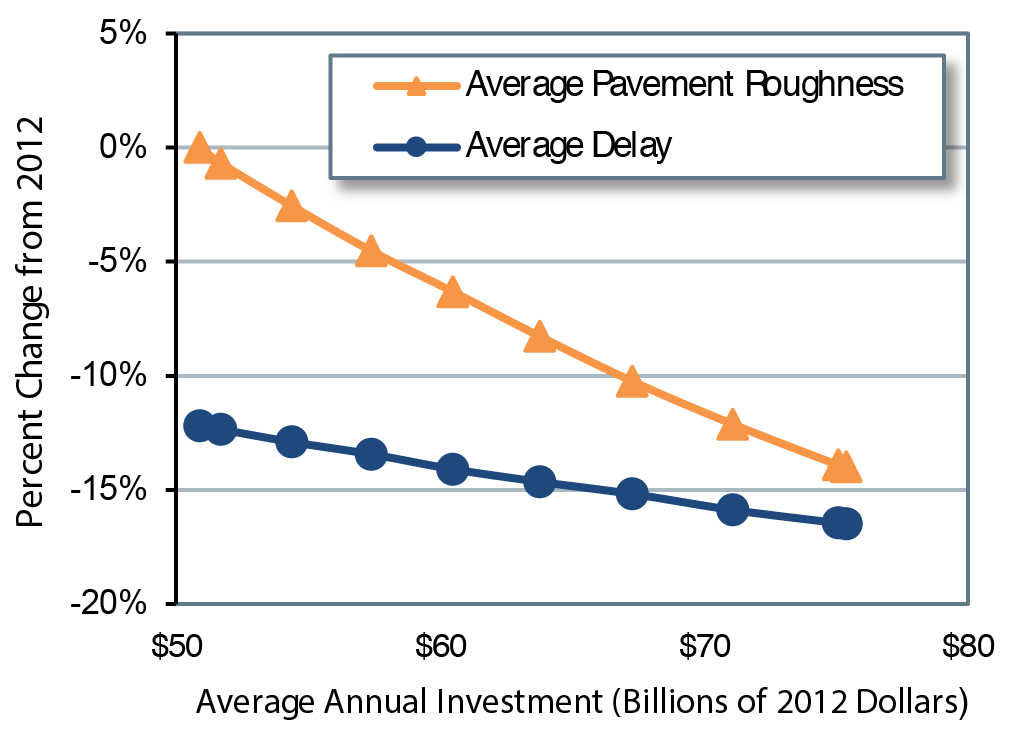
Sustaining HERS-modeled investment at $57.4 billion in constant-dollar terms over 20 years is projected to result in a 4.5-percent decrease in average pavement roughness per VMT and a 13.4-percent decrease in average delay by 2032 relative to 2012. HERS projects that constant-dollar spending growth of 2.53 percent per year would suffice to finance all cost-beneficial capital improvements on Federal-aid highways by 2032. This spending would translate into an average annual investment level of $75.4 billion and result in a 14.0-percent decrease in average pavement roughness and a 16.5-percent reduction in average delay per VMT.
Projected Change in 2032 Highway Conditions and Performance Measures Compared with 2012 Levels for Various Levels of Investment
Sustaining NBIAS-modeled investment at $16.4 billion in constant-dollar terms is projected to result in a reduction in the deck area-weighted share of structurally deficient bridges from 8.2 percent in 2012 to 2.9 percent in 2032. NBIAS projects that constant-dollar spending growth of 3.72 percent per year would suffice to eliminate the backlog of cost-beneficial capital improvements to bridges by 2032.
CHAPTER 7
Potential Capital Investment Impacts: Transit
The current level of investment in preservation and replacement of existing assets is insufficient to prevent the SGR backlog from growing by 2032. The backlog currently stands at $89.9 billion. Maintaining the current annual investment in preservation ($9.8 billion) over the next 20 years would result in a backlog that is 36 percent higher, $122.2 billion. The size of the projected 2032 backlog is sensitive to small variations in annual funding levels. For example, an average reduction of 2.5 percent in capital invested per year over 20 years would result in a backlog that is 81 percent higher, $162.5 billion.
Further, the one-time infusion of Recovery Act funds that began in 2009 might have inflated the assumed average annual investment over 20 years.
The condition of assets is determined using decay curves for each asset type and past maintenance and rehabilitation investments and utilization levels. The TERM assesses the aggregate average physical condition of all existing assets nationwide as of 2032. Nevertheless, even when overall conditions improve due to additional expenditures, some individual assets still will deteriorate.
The aggregate average condition rating of all nationwide transit assets in 2012 was 3.5, that is, in the middle of the range for "adequate" condition.
The current investment level of $9.8 billion per year is not sufficient to maintain the current aggregate average condition rating (3.5) in 2032. Instead, by 2032, the condition would decrease to 3.1, near the lower bound of the "adequate" range. Even higher levels of annual investment, however, still would result in average condition of existing assets below current levels. This outcome is due, in part, to assets for which the useful lives are much longer than the 20-year period of analysis. These assets include several new light-rail systems.
Transit capital investment in 2012 was at $17.1 billion. Preservation accounted for 58.5 percent , and expansion 41.5 percent . Urbanized areas with populations over 1 million accounted for 88 percent of all capital investment.
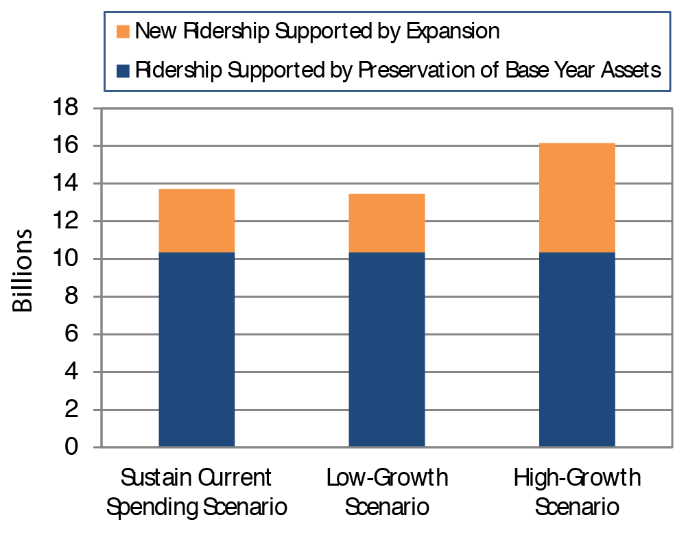
Impact of Expansion Investments on Transit Ridership — Basic Assumption: Maintain vehicle occupancy rates at current levels over the next two decades. The current level of investment in expansion ($7.1 billion) supports roughly 3.6 billion additional trips by 2032, which corresponds to an annual growth in ridership of 1.5 percent .
The current level of investment in expansion is insufficient to support forecasted ridership growth, leading to increased crowding on systems that currently experience high utilization. Increased crowding, in turn, could lead to increased dwell times, reduced operating speeds, and increased vehicle wear. Our demand forecasts predict an average annual rate of increase in ridership of 1.7 percent per year over 20 years: 2012—2032. An annual investment of $8.0 billion is required to keep the average rate of vehicle occupancy constant over this period.
CHAPTER 8
Selected Capital Investment Scenarios: Highways
This report presents a set of illustrative 20-year capital investment scenarios based on simulations developed using HERS and NBIAS, with scaling factors applied to account for types of capital spending that are not currently modeled. The scenario criteria were applied separately to the Interstate System, the NHS, Federal-aid highways, and the highway system as a whole.
The Sustain 2012 Spending scenario assumes that capital spending is sustained in constant-dollar terms at the 2012 level of $105.2 billion from 2013 through 2032. (In other words, spending would rise by exactly the rate of inflation during that period.)
The Maintain Conditions and Performance scenario assumes that capital investment gradually changes in constant-dollar terms over 20 years to the point at which selected measures of highway and bridge performance in 2032 are maintained at their 2012 levels. For the highway system as a whole, the average annual investment level associated with this scenario is $89.9 billion; this suggests that sustaining spending at the 2012 level of 105.2 billion should result in improved overall conditions and performance. Such is not the case for Interstate highways, as the $24.1-billion average annual investment level needed for the Maintain Conditions and Performance scenario is more than the $20.5 billion of capital spending on Interstate highways in 2012.
The Improve Conditions and Performance scenario assumes that capital investment gradually rises in constant-dollar terms to the point at which all cost-beneficial investments could be implemented by 2032. This scenario can viewed as an "investment ceiling," above which it would not be cost-beneficial to invest. Of the $142.5 billion average annual investment level under the Improve Conditions and Performance scenario, $85.3 billion (59.8 percent ) would be directed toward improving the physical condition of existing infrastructure assets (system rehabilitation); this portion is identified as the State of Good Repair benchmark. This scenario also includes $35.7 billion (25.1 percent ) directed toward system expansion and $21.5 billion (15.1 percent ) for system enhancement.
|
Average Annual Cost by Investment Scenario (Billions of 2012 Dollars) |
|||
|---|---|---|---|
| System Subset | Sustain 2012 Spending | Maintain C&P | Improve C&P |
| Interstate | $20.5 | $24.1 | $31.8 |
| NHS | $54.6 | $51.7 | $72.9 |
| Federal-aid Highways | $79.0 | $69.3 | $107.9 |
| All Roads | $105.2 | $89.9 | $142.5 |
In addition to addressing future highway and bridge needs as they arise over 20 years, the Improve Conditions and Performance scenario would address the estimated $830.0-billion existing backlog of cost-beneficial highway and bridge investments as of 2012. Approximately $156.8 billion (18.8 percent ) of the total backlog is for the Interstate System, $394.9 billion (47.2 percent ) is for the NHS, and $644.8 billion (77.1 percent ) is for Federal-aid highways.
CHAPTER 8
Selected Capital Investment Scenarios: Transit
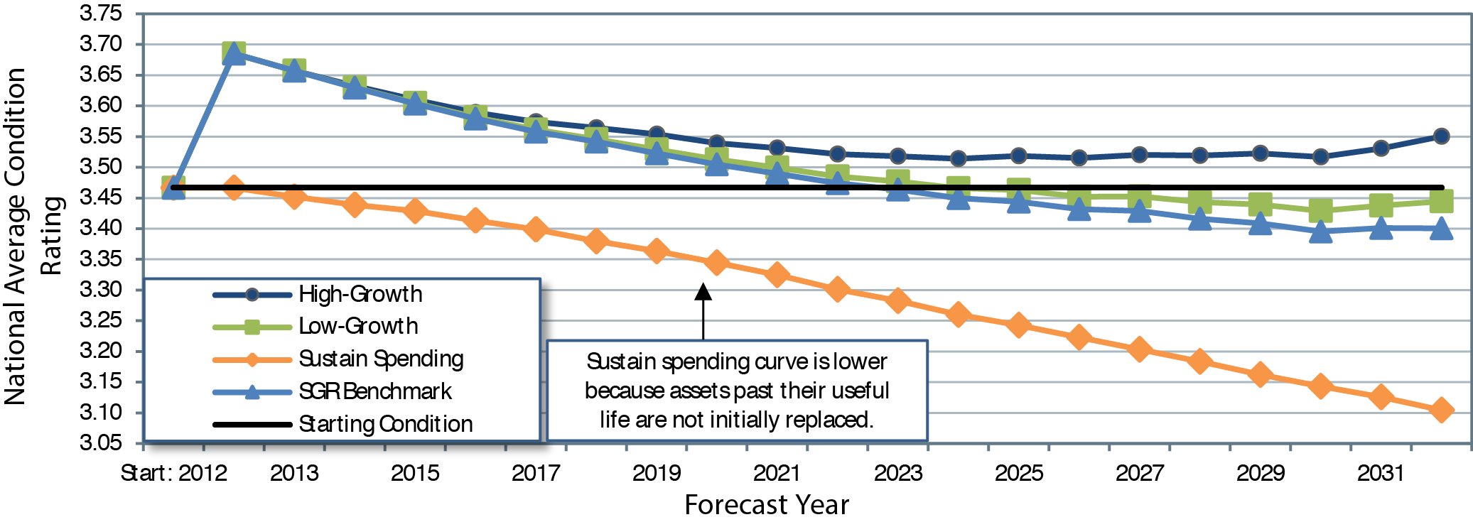
Chapter 8 explores the consequences of three distinct investment scenarios: maintaining current levels, meeting low-growth ridership levels, and meeting high-growth ridership levels. It also includes the SGR Benchmark.
Average Annual Investment 2013 through 2032
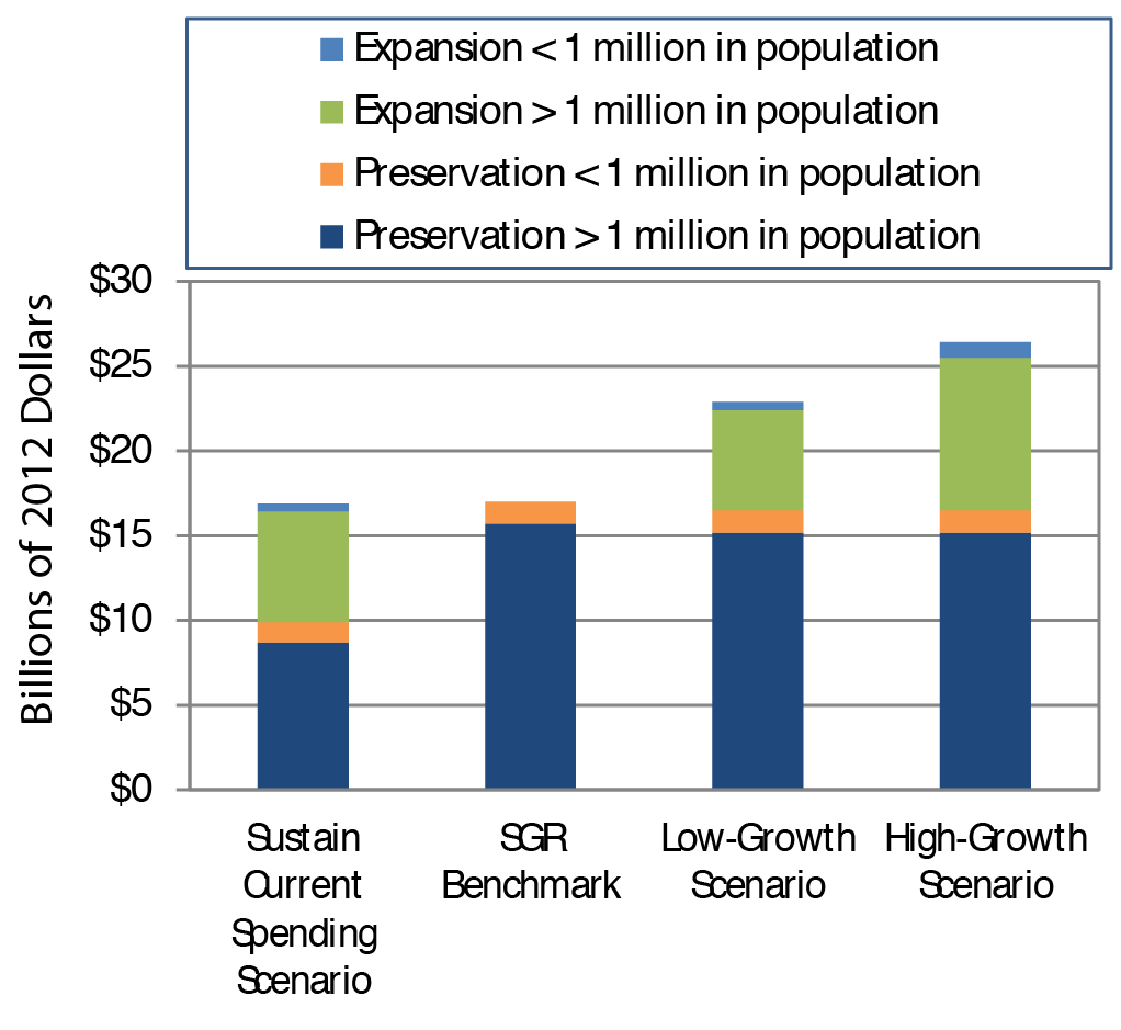
- Sustain 2012 Spending Scenario: Total spending under this scenario is well below that of the other needs-based scenarios, indicating that sustaining recent spending levels is insufficient to attain the investment objectives of the SGR Benchmark and the Low-Growth and High-Growth scenarios. This projection suggests future increases in the size of the SGR backlog and deterioration in the quality of service and likely increase in the number of transit riders per peak vehicle-including an increased incidence of crowding-in the absence of increased expenditures.
- SGR Benchmark: The level of expenditures required to attain and maintain an SGR over the upcoming 20 years-which covers preservation needs but excludes any expenditures on expansion investments-is 8.6 percent higher than that currently expended on asset preservation and expansion combined.
- Low- and High-Growth Scenarios: The level of investment to address expected preservation and expansion needs is estimated to be about 46 to 69 percent higher than the Nation's transit operators currently expend.
Projected Total Ridership Per Year
The share of transit assets exceeding their usual lives will increase if the level of investment over the next 20 years is maintained at 2012 levels. The proportion of existing asset categories exceeding their useful lives will undergo a near-continuous increase across each of these categories.
CHAPTER 9
Supplemental Scenario Analysis: Highways
The 2013 C&P Report presented two values for each scenario based on alternative assumptions about future VMT growth. The average annual investment level for the Maintain Conditions and Performance scenario ranged from $65.3 to $86.3 billion in 2010 dollars. Adjusting these values for inflation shifts this range to $69.3 to $91.6 billion in 2012 dollars. The comparable amount for this scenario presented in Chapter 8 of this edition is $89.9 billion in 2012 dollars, approximately 1.9 percent lower than the high end of the adjusted 2013 C&P Report range.
The 2013 C&P Report estimated an average annual investment range of $123.7 to $145.9 billion for the Improve Conditions and Performance scenario in 2010 dollars; adjusting for inflation increases this range to $131.3 to $154.9 billion in 2012 dollars. The comparable amount for the Improve Conditions and Performance scenario presented in Chapter 8 of this edition is $142.5 billion, toward the middle of the adjusted 2013 C&P Report range.
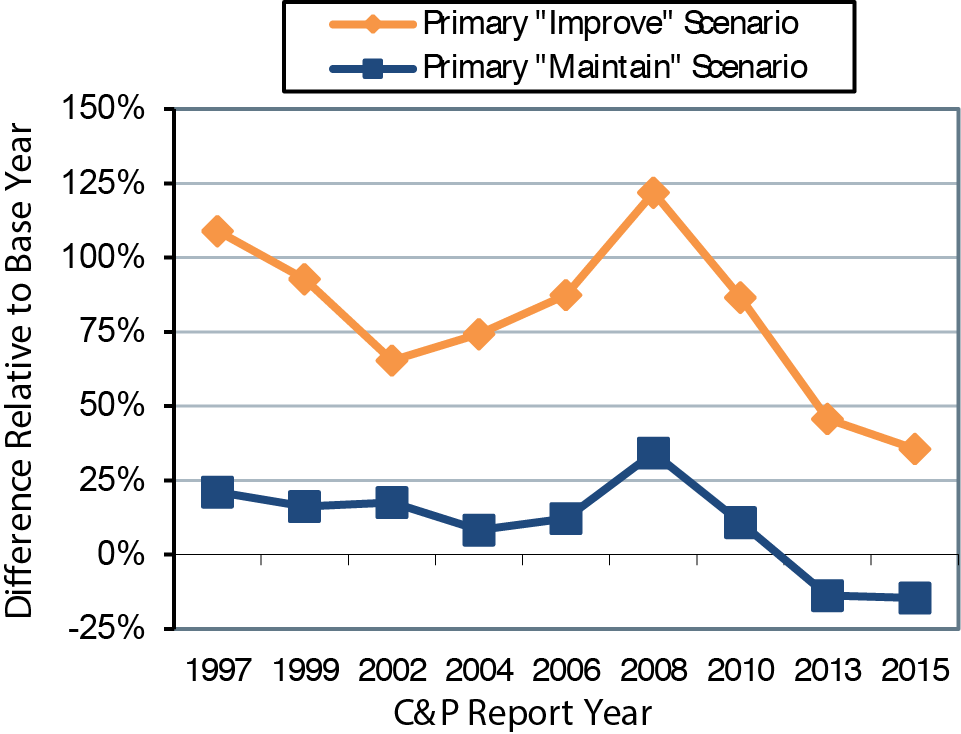
The names and definitions of the highway scenarios presented in the C&P report have varied over time, but each edition has generally included one primary scenario oriented toward maintaining the overall state of the system and one oriented toward improving the overall state of the system. Starting with the 1997 C&P Report, the "gap" between base-year spending and the average annual investment level for the primary "Maintain" and "Improve" scenarios has varied, rising as high as 34.2 percent and 121.9 percent , respectively, in the 2008 C&P Report (comparing needs in 2006 dollars with actual spending in 2006). These larger gaps coincided with a 43.3-percent increase in construction costs between 2004 and 2006. For the current 2015 C&P Report, the gap associated with the Improve Conditions and Performance scenario has fallen to 35.5 percent , while the gap with the Maintain Conditions and Performance scenario is negative (—14.6 percent ).
Gap Between Average Annual Investment Scenarios and Base Year Spending as Identified in the 1997 to 2015 C&P Reports
The decision to base the 2015 C&P Report scenarios on a national-level VMT forecast model rather than higher State-provided forecasts was driven in part by a review of the accuracy of the VMT forecasts used in previous C&P reports. States have tended to underpredict future VMT during periods when actual VMT was growing rapidly and to overpredict at times when actual VMT growth was slowing or declining.
CHAPTER 9
Supplemental Scenario Analysis: Transit
New technologies have had an impact on transit investment needs. As with most industries, the existing stock of assets used to support transit service is subject to ongoing technological change and improvement. Such change and improvements tend to increase investment costs. For example, by 2032, alternative, cleaner fuels are expected to propel more than 70 percent of the national bus fleet. These vehicles are more expensive to purchase and operate.
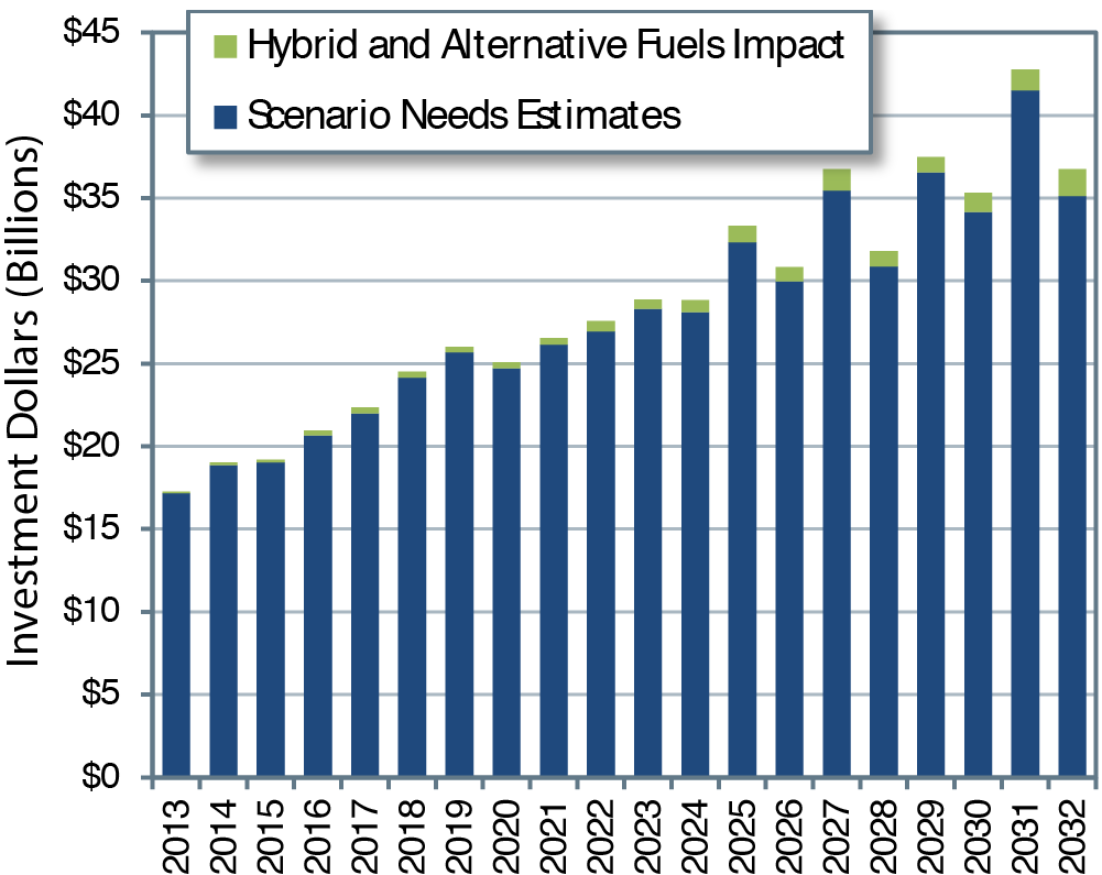
A cleaner, more fuel-efficient national bus fleet will not affect capital investment needs significantly over the next 20 years. The chart below adds the estimated additional funding required to support a national transit bus fleet composed of more than 70 percent alternative fuel vehicles in 2032 to the forecasted capital investment needs under the Low-Growth scenario.
Impact of Shift to Vehicles Using Hybrid and Alternative Fuels on Investment Needs: Low-Growth Scenario
If the levels of investment in preservation and expansion are kept the same as in 2012, the average condition of all assets will decline from the middle of the adequate range (3.5 in 2012) to 3.1, near the upper bound of the marginal range (2.0—2.9), in 2032.
Asset Condition Forecast for All Existing and Expansion Transit Assets
CHAPTER 10
Sensitivity Analysis: Highways
Sound practice in modeling includes analyzing the sensitivity of key results to changes in assumptions. Chapter 10 demonstrates how the baseline scenarios presented in Chapter 8 would be affected by changing some HERS and NBIAS parameters.
If VMT per capita were to remain constant from 2012 to 2032, VMT would grow by 0.74 percent per year (based on U.S. Census population projections), rather than the 1.04-percent annual rate assumed in the baseline analyses. This assumption would reduce the average annual investment level under the Improve Conditions and Performance scenario to $129.0 billion. If travel increases at the annual rates States project in the HPMS (1.41 percent ) and the NBI (1.46 percent ), the cost of this scenario would increase to $159.8 billion.
The valuation of travel time savings assumed in the baseline scenarios is linked to average hourly income; personal travel is valued at 50 percent of income, while business travel is valued at 100 percent . Alternative tests were run reducing these shares to 35 percent and 80 percent , respectively, and increasing them to 60 percent and 120 percent . Applying a lower value of time reduces the benefits associated with travel time savings and reduces the average annual investment level under the Improve Conditions and Performance scenario from $142.5 billion to $134.6 billion, as some potential projects would no longer qualify as cost beneficial. Assuming a higher value of time increases the annual cost of this scenario to $147.7 billion.
The baseline scenarios assume the value of a statistical life is $9.1 million when computing safety-related benefits. Reducing this value to $5.2 million would reduce the annual cost of the Improve Conditions and Performance scenario to $138.3 billion; increasing the value to $12.9 million would increase the annual cost to $144.2 billion.
Benefit-cost analyses use a discount rate that scales down benefits and costs arising later in the future relative to those arising sooner. The baseline scenarios assume a 7-percent rate; changing this to 3 percent would increase the average annual investment level under the Improve Conditions and Performance scenario to $171.5 billion.
| Impact of Alternative Assumptions on Highway Scenario Average Annual Investment Levels | ||
|---|---|---|
| Parameter Change | Maintain C&P | Improve C&P |
| (Billions of 2012 Dollars) | ||
| Baseline | $89.9 | $142.5 |
| Slower Growth in VMT | $81.3 | $129.0 |
| Faster Growth in VMT | $101.1 | $159.8 |
| Lower Value of Time | $84.7 | $134.6 |
| Higher Value of Time | $92.7 | $147.7 |
| Lower Value of Statistical Life | $89.0 | $138.3 |
| Higher Value of Statistical Life | $90.6 | $144.2 |
| 3 percent Discount Rate | $88.0 | $171.5 |
The impacts of alternative assumptions on the Maintain Conditions and Performance scenario are generally smaller and are linked to either the models' distribution of spending among different capital improvement types or to reduced VMT.
CHAPTER 10
Sensitivity Analysis: Transit
TERM relies on several key input values, variations of which can significantly influence the projections of capital needs for the scenarios considered in the C&P report: the SGR benchmark and Low-Growth and High-Growth scenarios.
Impact of alternative replacement condition thresholds on transit preservation needs-Baseline: Assets are replaced at a condition rating of 2.5. Analysis suggests that each scenario is sensitive to changes in the replacement condition threshold. The sensitivity increases disproportionately with higher replacement condition thresholds. For example, reducing the condition threshold to 2.0 tends to reduce the SGR backlog by $0.7 billion (4 percent ). In contrast, increasing the threshold to 3.0 increases preservation needs by more than $1 billion (6 percent ). Note that selecting a higher replacement condition results in asset replacement at an earlier age, which in turn results in more replacements over the 20-year forecast.
Impact of increase in capital costs on transit investment estimates. The asset costs used in TERM are based on actual prices agencies paid for capital purchases as reported to the FTA in the Transit Electronic Award Management system and in special surveys. Asset prices in the current version of TERM were converted from the dollar-year replacement costs in which assets were reported to FTA by local agencies (which vary by agency and asset) to 2012 dollars using the RSMeans© construction cost index. Any increase in capital costs without a similar increase in transit benefits results in lower benefit-cost ratios and failure of some investments to pass this test. The analysis shows that a 25-percent increase in capital costs for the Low-Growth and High-Growth scenarios would yield a roughly 13-percent and 15-percent increase, respectively, in capital needs that pass TERM's benefit-cost test.
Impact of alternative value of time rates on transit investment estimates. The most significant source of transit investment benefits as assessed by TERM's benefit-cost analysis is the net cost savings to users of transit services, a key component of which is the value of travel time savings. The current hourly rate based on U.S. Department of Transportation guidance is $12.50. Increasing this rate results in higher benefits, which results in including projects that failed the benefit-cost test at the standard rate. Decreasing the rate has the opposite effect. Doubling the rate (to $25.00) results in increases of 4.2 percent and 6.5 percent in capital needs for the Low-Growth and High-Growth scenarios, respectively. Reducing the rate by half (to $6.25) results in decreases of 12 percent and 13 percent , respectively.
Impact of discount rate. TERM's benefit-cost test is responsive to the discount rate used to calculate the present value of investment costs and benefits. TERM's analysis uses a rate of 7 percent in accordance with Office of Management and Budget guidance. The analysis using a rate of 3 percent (57 percent smaller) leads to an increase of 17.2-percent investment needs in the High-Growth scenario, but no change in the Low-Growth scenario.
CHAPTER 11
Pedestrian and Bicycle Transportation
DOT is committed to making walking and bicycling safer and more comfortable transportation options for everyone. The 1994 National Bicycling and Walking Study set a goal to double the percentage of trips made by bicycling and walking from 7.9 percent to 15.8 percent . This share had risen to 11.5 percent by 2009, just shy of halfway toward reaching this goal.
Bicycle and Pedestrian Travel Trends as Percentage of All Trips, 1994 and 2009
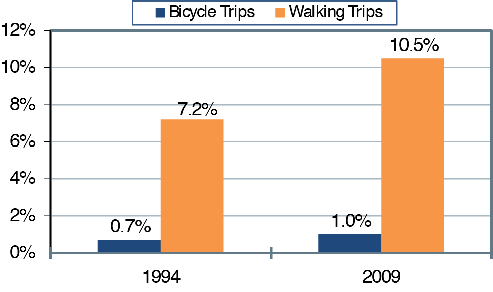
The 1994 study also set a goal of reducing pedestrian and bicycle injuries and fatalities by 10 percent . This goal has been exceeded, but recent trends indicate some reversal of progress, as injuries and fatalities have risen since 2009.
Federal funding for pedestrian and bicycle transportation has increased significantly, from $113 million in 1994 to a peak level of $1.2 billion in 2009; funding for 2014 was $820 million.
Federal policies and guidance supporting the inclusion of pedestrian and bicycle transportation in routine transportation planning, design, and construction have advanced multimodal planning and project development at all levels. Hundreds of communities, MPOs, and State Departments of Transportation (DOTs) have adopted Complete Streets policies, which require the formal consideration of all modes of travel throughout the project planning and development process. States and communities now routinely accommodate people with disabilities when developing pedestrian facilities and pedestrian access routes.
Context Sensitive Solutions, a collaborative, interdisciplinary, and holistic approach to the development of transportation projects, has become increasingly accepted by a broad range of stakeholders in all phases of program delivery, including long-range planning, programming, environmental studies, design, construction, operations, and maintenance.
The field of pedestrian and bicycle transportation engineering and planning has evolved, enabling practitioners at all levels to become more effective in improving safety and mobility for pedestrians and bicyclists. Professional organizations such as the Association of Pedestrian and Bicycle Professionals and pedestrian and bicycle advocacy organizations have played a key role in this process. Information-sharing resources such as the Pedestrian and Bicycle Information Center have been established, and professional training programs, guidebooks, and other educational resources have been developed.
CHAPTER 12
Transportation Serving Federal and Tribal Lands
The Federal government holds title to approximately 30 percent (650 million acres) of the total land area of the United States. Additionally, on behalf of Tribal governments, approximately 55 million acres of land is held in trust. Federal lands have many uses, including the facilitation of national defense, recreation, grazing, timber and mineral extraction, energy generation, watershed management, fish and wildlife management, and wilderness maintenance.
More than 450,000 miles of Federal roads provide access to Federal lands, creating opportunities for recreational travel and tourism, protection and enhancement of resources, and sustained economic development in both rural and urban areas. Annual visits to Federal lands total nearly 1 billion, and are expected to rise as the population increases, posing a challenge to Federal land management agencies in fulfilling their missions of providing visitor enjoyment while conserving precious resources. Accommodating growing traffic volumes and demands for visitor parking will require innovation and creative solutions.
| Roads Serving Federal Lands1 | ||||||||
|---|---|---|---|---|---|---|---|---|
| Federal Agency | Public Paved Road Miles | Paved Road Condition | Public Unpaved Road Miles | Public Bridges | Backlog of Deferred Maintenance2 | |||
| Good | Fair | Poor | Total | Structurally Deficient | ||||
| Forest Service | 9,500 | 42% | 55% | 3% | 362,500 | 4,200 | 11% | $2.9 billion3 |
| National Park Service | 5,500 | 59% | 29% | 12% | 4,100 | 1,442 | 3% | $6 billion |
| Bureau of Land Management | 500 | 65% | 20% | 15% | 600 | 835 | 3% | $350 million |
| Fish and Wildlife Service | 400 | 60% | 25% | 15% | 5,200 | 281 | 7% | $1 billion |
| Bureau of Reclamation | 762 | 65% | 25% | 10% | 1,253 | 331 | 12% | N/A |
| Bureau of Indian Affairs | 8,800 | N/A | N/A | N/A | 20,400 | 929 | 15% | N/A |
| Tribal Governments | 3,300 | N/A | N/A | N/A | 10,200 | N/A | N/A | N/A |
| Military Installations | 27,900 | N/A | N/A | N/A | N/A | 1,418 | 26% | N/A |
| U.S. Army Corps of Engineers | 5,247 | 56% | 30% | 14% | 2,549 | 416 | 6.20% | N/A |
|
1 Data shown are not for a consistent year, but instead reflect the latest available information as of late 2014 when these data were obtained from the FLMAs. Road condition categories are based on definitions of each, which are not fully consistent. Structural deficiencies are classified using a uniform definition consistent with that presented in Chapter 3. 2 Backlog includes only transportation-related amounts. 3 Value is for passenger car roads only. |
||||||||