prepared for
Federal Highway Administration
Office of Transportation Policy Studies
prepared by
Cambridge Systematics, Inc.
100 CambridgePark Drive, Suite 400
Cambridge, Massachusetts 02140
in association with
Battelle Memorial Institute
Columbus, Ohio
Battelle Subcontract No. 139189-32, Modification 02
March 19, 2007
Also available in PDF ![]() (4.23 MBs)
(4.23 MBs)
You will need the Adobe Reader to view the PDF.
Freight bottlenecks are an increasing problem today because they delay large numbers of truck freight shipments. They will become increasingly problematic in the future as the U.S. economy grows and generates more demand for truck freight shipments. If the U.S. economy grows at a conservative annual rate of 2.5 to 3 percent over the next 20 years, domestic freight tonnage will almost double and the volume of freight moving through the largest international gateways may triple or quadruple. Without new strategies to increase capacity, congestion at highway freight bottlenecks may impose an unacceptably high cost on the nation's economy and productivity.
The Texas Transportation Institute's (TTI) 2004 Urban Mobility Report estimates that the cost of congestion in 75 of the Nation's large urban areas in 2001 was $69.5 billion. Corresponding to that dollar loss is 3.5 billion hours of delay and 5.7 billion gallons of excess fuel consumed. However, the TTI methodology is based on analyzing mainline segments of highway rather than specific bottlenecks.
The Federal Highway Administration (FHWA) together with the Texas Transportation Institute currently uses the Highway Performance Monitoring System (HPMS) and the National Bridge Inventory (NBI) to estimate congestion. Neither HPMS nor NBI adequately reflect the influence of interchanges on highway capacity. The HPMS contains data on the through-lane capacity but does not account for the reduced capacity caused by weaving and merging movements at interchanges. In fact, interchanges are not even explicitly identified in the HPMS. The NBI does contain data on bridges located at interchanges but it does not include detailed information about the interchanges and NBI does not treat interchange bridges separately from other bridges. In short, the two data systems and the models based on those systems (Highway Economic Requirements System and TTI's congestion model) do not support the estimation of interchange congestion impacts. Further, congestion often extends well beyond the locus of the interchange.
This data/methodology gap was discovered as part of the An Initial Assessment of Freight Bottlenecks on Highways1. Using a Bottleneck Delay Estimator developed by Cambridge Systematics (CS) for the American Highway Users Alliance2, CS developed preliminary estimates of the truck hours of delay on the "critical leg" of each interchange based on information from the HPMS database.
This previous analysis of freight (highway) bottlenecks shows a highly skewed distribution of bottlenecks -- primarily interchanges on urban Interstate highways -- accounting for 50 percent of the delay hours. However, the truck delay estimates are incomplete because the HPMS database does not have sufficiently detailed data to calculate (1) the delay effects of merge and weave areas at the interchanges, and (2) delays accrued by trucks in the other legs of the interchanges. The objective of this project is to conduct a feasibility study to determine how to model the delay associated with highway interchanges and then develop an interchange bottleneck delay estimator that can be applied to the national list of significant highway interchange bottlenecks.
This study builds on the work performed in Reference (1). In that study, truck bottlenecks were defined by a combination of three features: the type of constraint, the type of roadway, and the type of freight route. Table 1.1 shows how these three features were combined.
| Bottleneck Type Constraint |
Bottleneck Type Roadway |
Bottleneck Type Freight Route |
National Annual Truck Hours of Delay, 2004 (Estimated) |
|---|---|---|---|
| Interchange | Freeway | Urban Freight Corridor | 123,895,000 |
| Subtotal 123,895,000* | |||
| Steep Grade | Arterial | Intercity Freight Corridor | 40,647,000 |
| Steep Grade | Freeway | Intercity Freight Corridor | 23,260,000 |
| Steep Grade | Arterial | Urban Freight Corridor | 1,509,000 |
| Steep Grade | Arterial | Truck Access Route | 303,000 |
| Subtotal 65,718,000‡ | |||
| Signalized Intersection | Arterial | Urban Freight Corridor | 24,977,000 |
| Signalized Intersection | Arterial | Intercity Freight Corridor | 11,148,000 |
| Signalized Intersection | Arterial | Truck Access Route | 6,521,000 |
| Signalized Intersection | Arterial | Intermodal Connector | 468,000 |
| Subtotal 43,113,000‡ | |||
| Lane Drop | Freeway | Intercity Freight Corridor | 5,221,000 |
| Lane Drop | Arterial | Intercity Freight Corridor | 3,694,000 |
| Lane Drop | Arterial | Urban Freight Corridor | 1,665,000 |
| Lane Drop | Arterial | Truck Access Route | 41,000 |
| Lane Drop | Arterial | Intermodal Connector | 3,000 |
| Subtotal 10,622,000‡ | |||
| Total 243,032,000 |
One of the major results of this study verified previous notions about truck bottlenecks – that urban interchanges heavily used by weekday commuters represent the overwhelming source of delay for trucks. However, the methodology used to estimate delay and perform the rankings is a very simple scanning level of analysis. Given the importance of these types of bottlenecks, a more rigorous delay analysis was decided upon and the results are presented herein.
A study performed for the Ohio Department of Transportation3 expanded on the bottleneck analysis approach used in both the AHUA and previous FHWA studies. On freeways, the AHUA study found that the predominant type of bottleneck was freeway-to-freeway interchanges. Lane-drop bottlenecks were far less common and interchanges with surface streets produced significantly less delay than freeway-to-freeway interchanges. The AHUA methodology (used also in the previous FHWA bottleneck study) is based on identifying the "critical leg" of a freeway-to-freeway interchange (i.e., one of the two intersecting highways for the interchange) and assumes that all interchange delay is attributable to that leg. (Lane-drop and freeway-to-surface-street bottlenecks do not need this assumption since there is only one freeway "leg" present. In the AHUA approach, delay is estimated using a set of equations developed from a queuing-based model; these are the same equations that are in FHWA's Highway Economic Requirements (HERS) model. This provides a good first-cut for identifying bottlenecks but delay is highly dependent on the actual interchange configurations (roadway geometry) at each location. For the Ohio work, the methodology was extended by:
The Ohio methodology is therefore more closely aligned with an operational-level analysis similar to those in the Highway Capacity Manual. It identifies specific merge points within each interchange that are the causes of delay (usually, not all merge points are problems) rather than using the planning-level notion of a "critical leg". Figure 1.1 details the Ohio methodology for determining truck demand at each bottleneck.
The approach taken for the present study was intermediate in complexity and data requirements between the AHUA and Ohio methodologies. The specifics of the methodology follow.
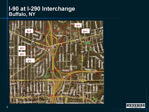
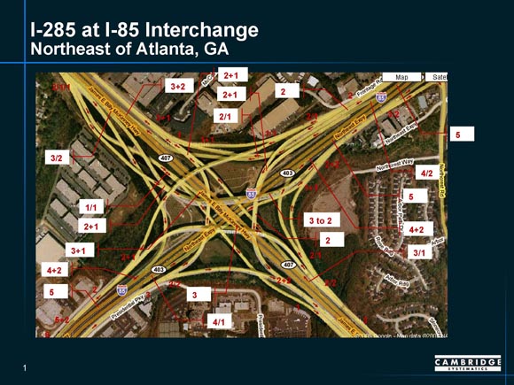
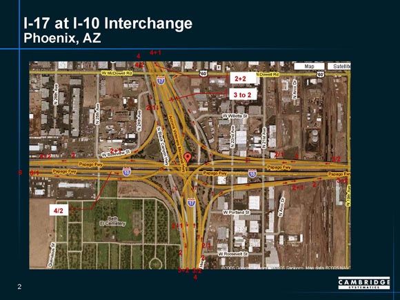
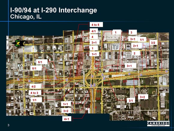
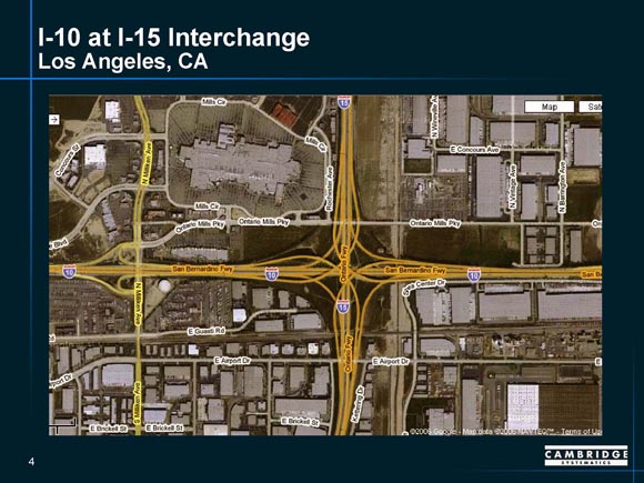
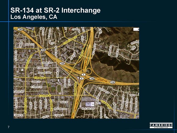
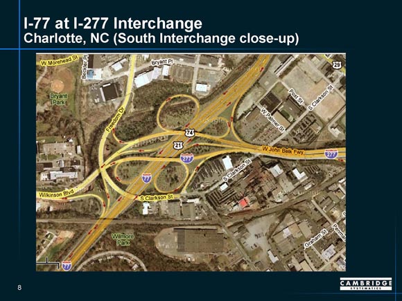
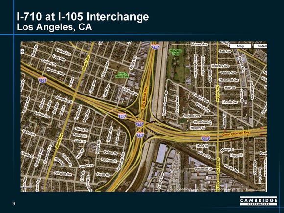
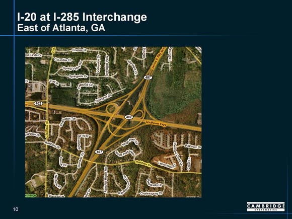
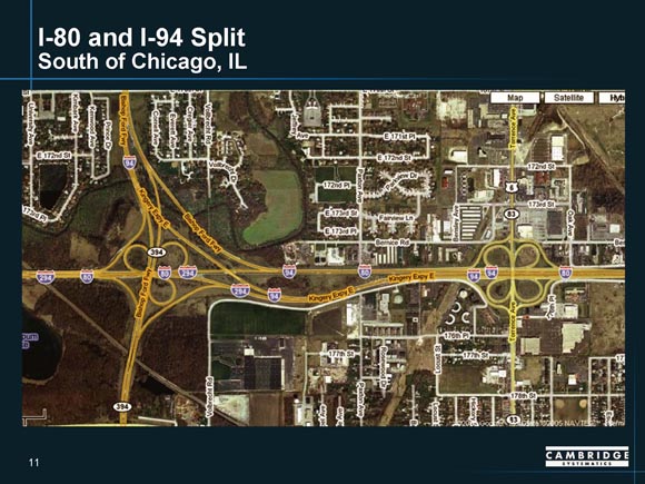
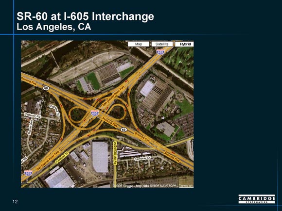
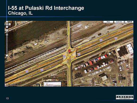
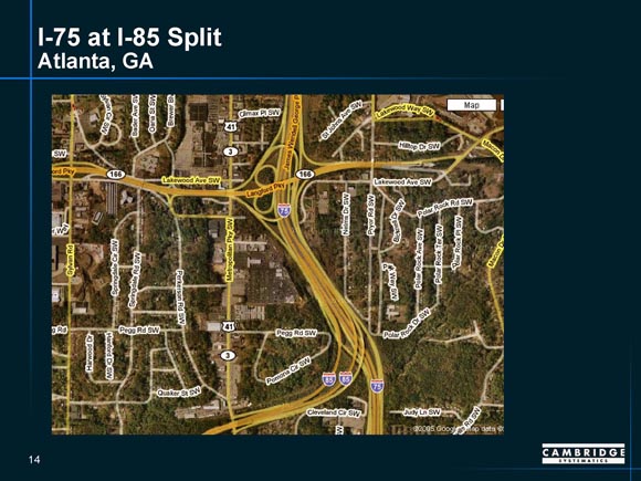
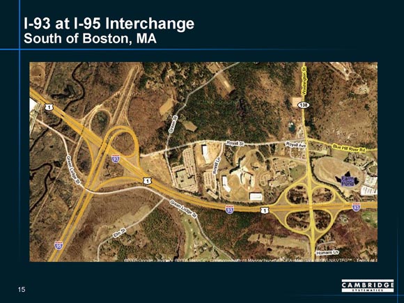
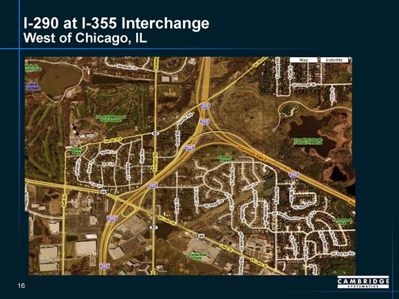
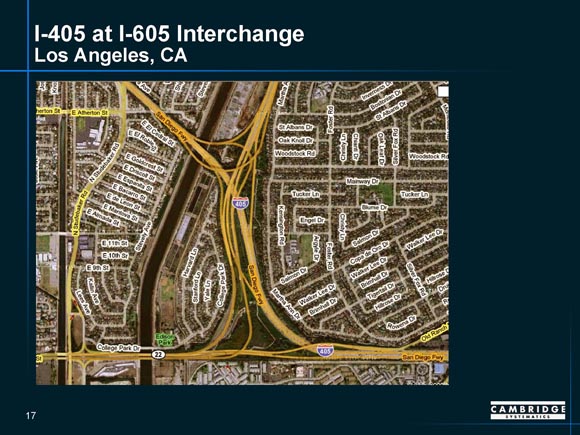
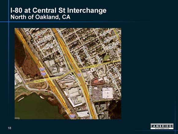
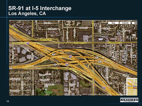
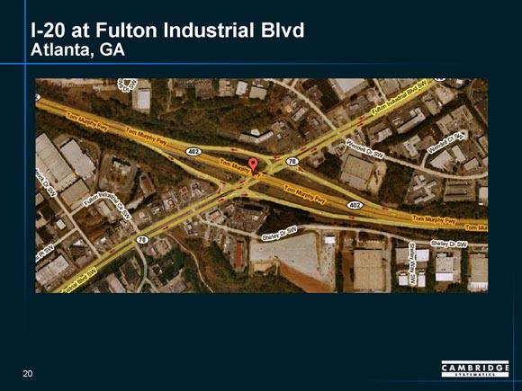
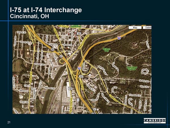
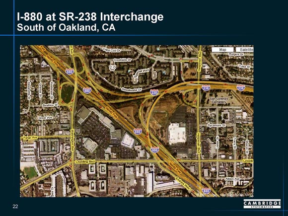
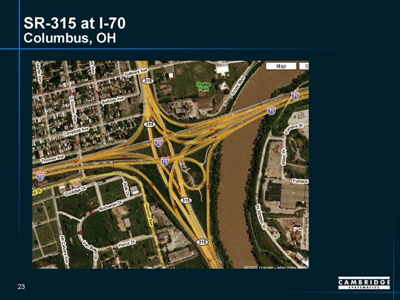
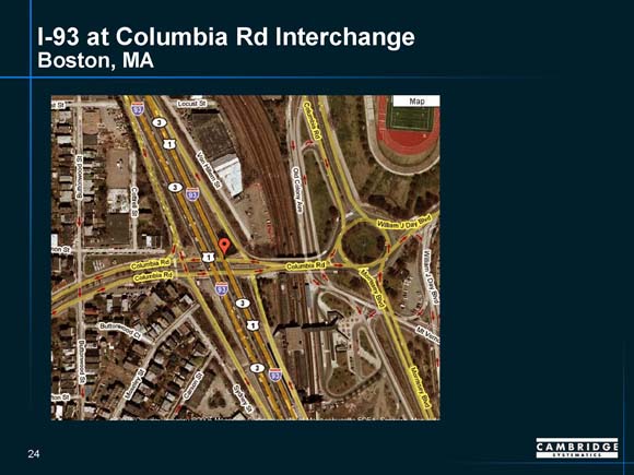
Interchange configurations and geometrics were obtained using the satellite-based photos available from GoogleEarth.4 Figure 2.1 shows an example of the photos available; Appendix A5 shows the photos for all the interchanges studied. Figure 2.1 is still at a relatively low resolution rate - more detailed resolutions are available that allow determining the number of lanes at specific points. (Indeed, even individual vehicles can be ascertained, even down to telling if they are a car, truck, or large truck!)
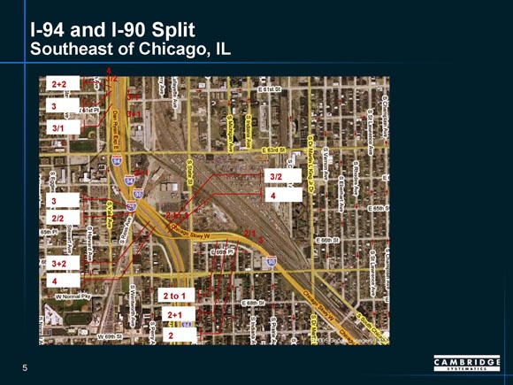
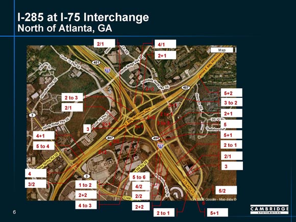
For each interchange, the key merge points where traffic is moving away from the center of the interchange were identified. At each merge point, the number of entering and exiting lanes was noted. If there was a change in the number of exiting lanes within 1,500 feet of the interchange, this too was noted. The capacity of each merge juncture was determined by the minimum of either the number of exiting lanes or the number of lanes 1,500 feet downstream. Table 2.1 shows the basic information used at each merge juncture. The interchange configuration information used in this study is therefore as detailed as that used in the Ohio study.
As shown in Appendix A, the design (ramp configuration) of many of the interchanges is extremely complex. For that reason, some of the interchanges exhibit multiple ramp merges for a particular "exit" (i.e., travel direction away from the interchange).
The detailed traffic data available for the Ohio study were not available for this study. The scope of this study did not allow for the contact of other DOTs and assembly of the data. Further, it is not known if other DOTs maintain counts, especially vehicle classification counts, on freeway-to-freeway ramps. Therefore, a simpler method was developed. AADTs for all the approaches of the interchanges were identified from the HPMS Universe data using the LRS Beginning and Ending Points. Because the HPMS Universe data provides continuous coverage of highway segments, there were no gaps the highway segments used for this analysis. Identifying which HPMS segments were located immediately prior to the interchange involved some judgment, with the LRS information being used to get close to the interchange, then looking for large changes in AADTs indicating that merging and diverging traffic flow was occurring. Once AADTs (two-way) for each approach were identified, it was assumed that the directional AADT was half of the total AADT.6 Turning movements were then synthetically derived using the balancing procedure first identified in NCHRP 255 and in widespread use among travel demand modelers. Turning movements were then assigned to each ramp.
| BOTTLENECK NAME | Exiting Direction | Pct. Trucks | Ramp-to-Ramp Dir AADT |
Ramp-to-Ramp No. Lanes |
Ramp-to-Mainline Dir AADT |
Ramp-to-Mainline No. Lanes |
|---|---|---|---|---|---|---|
| I-90 at I-290 in Buffalo | NB | 0.24 | 67614 | 4 | 67614 | 4 |
| SB | 0.10 | 65871 | 2 | 65871 | 3 | |
| EB | 0.10 | 67614 | 2 | |||
| NB | 0.24 | 67614 | 4 | 67614 | 4 | |
| I-17 at I-10 in Phoenix | EB | 0.13 | 51516 | 2 | 121130 | 6 |
| WB | 0.13 | 51516 | 2 | 121130 | 6 | |
| NB | 0.11 | 61499 | 4 | |||
| SB | 0.11 | 73016 | 3 | 104499 | 5 | |
| I-285 at I-85 in Atlanta | EB | 0.13 | 59836 | 126020 | 6 | |
| EB | 0.13 | 35100 | 2 | |||
| EB | 0.13 | 60836 | 4 | 127020 | 7 | |
| WB | 0.13 | 68251 | 4 | 134435 | 6 | |
| NB | 0.13 | 39896 | 3 | |||
| NB | 0.13 | 73996 | 4 | 134495 | 6 | |
| NB | 0.13 | 133495 | 5 | |||
| SB | 0.13 | 55091 | 4 | 115590 | 5 | |
| SB | 0.13 | 26736 | 2 | |||
| I-90/94 at I-290 in Chicago | EB | 0.11 | 57278 | 2 | 102050 | 5 |
| EB | 0.11 | 102050 | 4 | |||
| WB | 0.11 | 34989 | 2 | |||
| WB | 0.11 | 58278 | 2 | 103050 | 4 | |
| NB | 0.05 | 46578 | 2 | 117300 | 4 | |
| NB | 0.05 | 46578 | 2 | 117301 | 4 | |
| SB | 0.05 | 67978 | 3 | 138700 | 5 | |
| SB | 0.05 | 67978 | 3 | 138700 | 5 | |
| I-15 at I-10 in Los Angeles | EB | 0.20 | 58068 | 5 | 123000 | 5 |
| WB | 0.20 | 117500 | 7 | |||
| WB | 0.20 | 52568 | 5 | 117500 | 7 | |
| NB | 0.11 | 58068 | 4 | 105000 | 6 | |
| SB | 0.11 | 53068 | 5 | 100000 | 5 | |
| SB | 0.11 | 100000 | 5 | |||
| I-90 at I-94 split in Chicago | NB | 0.12 | 118750 | 4 | ||
| SB | 0.12 | 23850 | 4 | |||
| I-75 at I-285 in Atlanta | EB | 0.13 | 19145 | 2 | ||
| EB | 0.13 | 49016 | 2 | 82795 | 7 | |
| EB | 0.13 | 81795 | 5 | |||
| WB | 0.13 | 73382 | 2 | 107161 | 4 | |
| NB | 0.13 | 47651 | 4 | |||
| NB | 0.13 | 77522 | 4 | 175614 | 7 | |
| SB | 0.13 | 28730 | 2 | |||
| SB | 0.13 | 46875 | 3 | 144964 | 6 | |
| SR-134 at SR-2 in Los Angeles | EB | 0.03 | 121999 | 5 | ||
| WB | 0.03 | 88615 | 5 | |||
| WB | 0.03 | 109500 | 6 | |||
| NB | 0.12 | 48972 | 2 | 72497 | 6 | |
| NB | 0.12 | 48975 | 2 | 72497 | 6 | |
| SB | 0.12 | 44159 | 4 | |||
| SB | 0.12 | 59500 | 5 | |||
| I-710 at I-105 in Los Angeles | EB | 0.16 | 26466 | 6 | 75116 | 6 |
| EB | 0.16 | 99000 | 6 | |||
| WB | 0.16 | 109500 | 5 | |||
| WB | 0.16 | 29966 | 4 | 78616 | 5 | |
| NB | 0.05 | 52850 | 2 | 113500 | 5 | |
| NB | 0.05 | 24884 | 2 | |||
| SB | 0.05 | 56350 | 3 | 117000 | 6 | |
| SB | 0.05 | 26466 | 2 | |||
| I-20 at I-285 in Atlanta | EB | 0.14 | 39715 | 3 | 84335 | 5 |
| EB | 0.14 | 39715 | 3 | 84335 | 5 | |
| WB | 0.14 | 63936 | 4 | |||
| WB | 0.14 | 82285 | 4 | |||
| NB | 0.10 | 37697 | 4 | 71199 | 6 | |
| NB | 0.10 | 37697 | 4 | 71199 | 6 | |
| SB | 0.10 | 39683 | 2 | 73185 | 4 | |
| SB | 0.10 | 39683 | 2 | 73185 | 4 | |
| I-80 at I-94 split in Chicago | EB | 0.18 | 57364 | 2 | 66247 | 4 |
| WB | 0.18 | 45191 | 2 | 50000 | 3 | |
| NB | 0.18 | 21364 | 2 | |||
| NB | 0.18 | 30250 | 3 | |||
| SB | 0.18 | 58450 | 2 | |||
| SB | 0.18 | 30916 | 2 | 57450 | 2 | |
| SR-60 at I-605 in LA | EB | 0.15 | 100740 | 4 | 131500 | 6 |
| WB | 0.15 | 99740 | 4 | 130500 | 5 | |
| NB | 0.12 | 85236 | 6 | 116527 | 5 | |
| NB | 0.12 | 116527 | 5 | |||
| SB | 0.12 | 85236 | 5 | 116527 | 6 | |
| I-55 at Pulaski in Chicago | EB | 0.15 | 4734 | 1 | 89017 | 3 |
| WB | 0.15 | 4734 | 1 | 89017 | 3 | |
| NB | 0.15 | 2634 | 2 | |||
| SB | 0.15 | 2634 | 2 | |||
| I-75 at I-85 in Atlanta | NB | 0.07 | 144700 | 6 | ||
| SB | 0.07 | 325000 | 12 | |||
| I-93 at I-95 in Boston (South) | EB | 0.14 | 75550 | 4 | ||
| WB | 0.14 | 77896 | 3 | |||
| SB | 0.14 | 77896 | 3 | |||
| SB | 0.14 | 77896 | 3 | |||
| I-290 at I-355 in Chicago | EB | 0.08 | 72600 | 4 | ||
| NB | 0.08 | 94100 | 5 | |||
| SB | 0.08 | 85100 | 3 | |||
| I-405 at I-605 in LA | NB | 0.15 | 157058 | 5 | 160000 | 6 |
| SB | 0.15 | 2219 | 2 | |||
| EB | 0.15 | 129933 | 7 | 131000 | 8 | |
| WB | 0.15 | 2219 | 1 | 132152 | 5 | |
| I-75 at I-74 in Cincinnati | WB | 0.10 | 59000 | 3 | 0 | 4 |
| WB | 0.10 | 0 | 3 | 0 | 4 | |
| SB | 0.12 | 0 | 2 | 89516 | 4 | |
| NB | 0.12 | 0 | 1 | 78000 | 3 | |
| I-880 at SR-238 in Oakland | EB | 0.12 | 22471 | 3 | 42000 | 3 |
| SB | 0.10 | 121000 | 5 | |||
| NB | 0.10 | 101524 | 5 | 123000 | 5 | |
| SR-315 at I-70 in Columbus | EB | 0.12 | 0 | 3 | 79557 | 4 |
| WB | 0.12 | 26254 | 2 | 63646 | 4 | |
| SB | 0.12 | 52379 | 2 | 67279 | 4 | |
| NB | 0.12 | 24999 | 2 | 18775 | 3 | |
| I-93 at I-90 in Boston | EB | 0.08 | 47737 | 2 | ||
| WB | 0.08 | 55313 | 3 | |||
| SB | 0.07 | 92192 | 4 | |||
| NB | 0.07 | 93578 | 4 | |||
| I-80 @ I-580/I-880 Oakland, CA | NB | 0.14 | 143500 | 4 | 143500 | 5 |
| NB | 0.09 | 143500 | 4 | 143500 | 5 | |
| WB | 0.09 | 194947 | 7 | |||
| EB | 0.09 | 55000 | 5 | |||
| I-77 @I-277 in Charlotte, NC (South) | NB | 0.17 | 10053 | 1 | 59445 | 4 |
| SB | 0.17 | 21579 | 1 | 71209 | 3 | |
| NB | 0.17 | 2007 | 1 | |||
| SB | 0.17 | 58203 | 2 | |||
| EB | 0.17 | 28946 | 4 | |||
| EB | 0.17 | 17209 | 3 |
Truck percents were obtained from two sources. First, for the dominant route in the interchange name (i.e., the first route number in the name), truck percents were obtained from the FAF-based assignments from Reference (1). For all other routes, truck percents were obtained from the HPMS Sample data.
Background
This study uses the delay equations developed in a previous FHWA study7 and subsequently adapted for use in the HERS model. A series of these equations were developed specifically to estimate the delay due to recurring bottlenecks. A brief history of the development of this methodology follows.
The equations were developed by using a simple queuing-based model. The procedure works as shown in Figure 2.2:
Note that this method considers the effect of delay from the interaction of demand and physical capacity only (usually termed "recurring" delay). It does not include or estimate incident related delay.
The basis of the model is the definition of capacity. If a highway section has a reduced capacity from "normal" (e.g. , due to weaving or other geometric constraint), then this reduced capacity must be used in the application of this model. Essentially, it treats all bottlenecks the same – just with varying values of capacity. This assumption will miss some of the operational nuances of certain types of conditions (weaves) when flows are restricted but still above level of service F (forced flow); after breakdown occurs, then the queuing procedure probably captures the effects adequately.
So, the concepts of highway capacity are used as a starting point, the resulting delay estimates are higher using this method than if HCM-based methods are used. Because the equations consider queuing, and HCM methods do not, these equations will predict more delay than HCM methods. Note that the HCM recommends that queuing procedures be used for oversaturated conditions, but does not provide a specific method. For example, in Chapter 25 ("Ramp and Ramp Junction"), it simply states that LOS F exists "when demand exceeds capacity". There are no explicit delay calculations for the various degrees of LOS F.
Most of the interchanges studied are of very high design standards with no weaving areas, but there are a few (see Appendix A for interchanges have weaving areas). These weaves were ignored, and analysis focused on the merge junctures as the capacity control for a particular turning movement. Also, note that even though the HCM procedure is complex and requires unavailable data, it still measures delay crudely as one of the LOS categories. This paper recommends efforts should be made to consider weaving areas in the future. This is especially important for future analysis that may move away from the major commuter bottlenecks and include poorly designed interchanges with weaves.
However, to date field data have been lacking to validate this procedure. Also, there is some indication that the traffic variability component is too large for congested highways - day-to-day variability is smaller on congested highways. (The traffic distributions on which the procedure is based are now 15 years old). The HERS model uses this procedure and FHWA staff are aware of the need to re-think the traffic distributions and to perform at least limited field testing of the procedure.
A comparison of the capabilities of the method used in this study and the Ohio study appear in Table 2.2. Also, the delay results for two bottlenecks common to both studies appear in Table 2.2. The overall delay calculations are close, but the current method estimates slightly higher delay at both interchanges. The truck delays are noticeably different, due to the different sources of truck volume information. In the current study, percentages from FAF are used (from the previous FHWA freight bottleneck study) whereas in the Ohio study, actual counts of trucks (by the FHWA 13-class scheme) were used.
Application to the Current Study
The equations relate the AADT-to-capacity ratio to delay. Directional AADTs were obtained as described above. One-way capacities were calculated using a base capacity of 2,400 pcphpl, adjusted downward for the percentage of trucks at each merge juncture. If there is a lane-drop either at the merge juncture or a 1000 feet downstream, that is included in the analysis; these lane-drops are considered part of the interchange. Other lane-drops (such as those at bridges) are not interchange-related and have been identified in the previous FHWA freight bottleneck study as "general capacity-related bottlenecks"
The equations for estimating total daily delay for each direction were applied to each merge juncture, then, the higher delay was chosen. The travel time without queuing factors (Hu) is small in comparison to those for queuing (Hr). Total delay for each merge juncture is then:
Total Delay at Merge Juncture = (Hu * VMT) + (Hr * AADT)
| Technical Aspect | Current Methodology | Ohio Methodology |
|---|---|---|
| Analysis of individual merge areas | Yes | Yes |
| Ramp volumes | Derived synthetically from inflow/outflow volumes | Measured directly |
| Truck volumes | FAF percentages | Measured directly |
| Delay estimation | Uses HERS equations | Applies queuing procedure directly at each ramp juncture |
| Total Annual Delay (hrs) | ||
| SR-315 at I-70 in Columbus | 3,062,600 | 2,938,500 |
| I-75 at I-74 in Cincinnati | 2,589,200 | 1,923,00 |
| Total Truck Delay (hrs) | ||
| SR-315 at I-70 in Columbus | 367,500 | 254,000 |
| I-75 at I-74 in Cincinnati | 305,800 | 166,250 |
VMT is calculated by multiplying AADT by ½ mile, assuming this is the distance traveled by vehicles as they pass through the interchange. Truck delay is obtained by multiplying total delay by percent trucks. This is clearly a simplifying assumption since it is assumed that the temporal distribution of trucks (hourly volumes) follow the same pattern as for total traffic.
Note that for this study, only ramp junctures were considered. An assessment of the interchanges at hand revealed that there were only two interchanges with weaving areas, mainly because these interchanges were designed to high standards.9 The two interchanges are:
In some cases, interchanges are constructed so that two ramps handling turning movements merge, then the combined ramp merges with through traffic on the mainline. In such cases, the higher delay (rather than the sum was chosen) because when two bottlenecks are closely spaced, one will control the operation. Therefore, only one delay value for each exiting direction is used. Figure 2.2 shows the equations for estimating the delay factors. Total delay for the interchange is then summed over all exiting directions for the interchange.
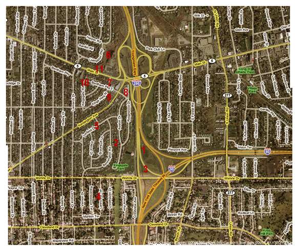
Figure 2.3 shows an example of what the analysis reveals at an individual interchange. Note that only two merge junctures create delay problems.10 These results are very typical – not all ramps and turning problems are bottlenecks at an interchange. Appendix B shows the delay results for each of the exiting directions at the interchanges.
Limitations of the Methodology
The goal of this project was to see if a cost-effective methodology could be developed for analyzing bottlenecks that is based on the specific physical restrictions of complex types of bottlenecks (interchanges). Generally, as analytic procedures become more detailed, their replication of reality will increase in accuracy and fewer assumptions have to be made, but the data requirements and operation become more onerous. For bottleneck analysis, the methods range from:
The methodology used here falls between these two ends of the spectrum, closer to the AHUA methodology because it is still a "planning level" analysis (in HCM terms). The major limitations of the methodology are as follows.
|
A.M. Peak Direction, 24-hour Delay Travel Time without Queuing (hours per vehicle mile)
Hu = 1 / Speed = ( 1 / Sf ) ( 1 + 5.44E-12 * X10)
for X <= 8
Hu = 1 / Speed = ( 1 / Sf ) ( 1.23E+00 - 7.12E-02 * X + 6.78E-03 * X2 - 1.83E-04 * X3)
for X > 8
Delay Due to Recurring Queues (hours per vehicle using the bottleneck) Hr = RECURRING DELAY = 0
for X <=8
Hr = RECURRING DELAY = 6.77E-03 * (X-8) - 4.13E-03 * (X -8)2 + 1.29E-03 * (X-8)3
for X > 8
P.M. Peak Direction, 24-hour Delay Travel Time without Queuing (hours per vehicle mile)
Hu = 1 / Speed = ( 1 / Sf ) ( 1 + 7.37E-12 * X10)
for X <= 8
Hu = 1 / Speed = ( 1 / Sf ) ( 1.13E+00 - 4.39E-02* X + 4.68E-03 * X2 1.32E-04 * X3)
for X > 8
Delay Due to Recurring Queues (hours per vehicle using the bottleneck) Hr = RECURRING DELAY = 0
for X <=8
Hr = RECURRING DELAY = 4.11E-03 * (X-8) + 1.26E-03 * (X-8)2 + 4.03E-04 * (X- 8)3
for X > 8
where: Sf = free flow speed = 60 mph
X = AADT/C
|
The bottleneck delay results from this study are compared to those from Reference (1) in Table 3.1. The bottlenecks are listed in order from the highest to the lowest based on the current delay estimates.
| Bottleneck Name | Annual Delay (hrs) Current Study Total |
Annual Delay (hrs) Current Study Truck |
Annual Delay (hrs) Previous FHWA Freight Bottleneck Study Truck |
|---|---|---|---|
| I-405 at I-605 in Los Angeles, CA | 19,363,000 | 2,662,600 | 1,245,500 |
| SR-60 at I-605 in Los Angeles, CA | 17,004,600 | 2,400,200 | 1,314,600 |
| I-75 at I-285 in Atlanta, GA | 17,330,400 | 2,253,000 | 1,497,300 |
| I-55 at Pulaski in Chicago, IL | 12,590,600 | 1,888,600 | 1,300,400 |
| I-80 @ I-580/I-880 Oakland, CA | 17,192,800 | 1,838,700 | 1,196,700 |
| I-285 at I-85 in Atlanta, GA | 13,962,100 | 1,815,100 | 1,641,200 |
| I-90/94 at I-290 in Chicago, IL | 22,427,800 | 1,600,300 | 1,544,900 |
| I-80 at I-94 split in Chicago, IL | 7,585,300 | 1,365,300 | 1,343,600 |
| I-15 at I-10 in Los Angeles, CA | 7,248,200 | 1,308,300 | 1,522,800 |
| I-880 at SR-238 in Oakland, CA | 11,951,400 | 1,200,300 | 1,106,700 |
| I-90 at I-290 in Buffalo, NY | 6,563,400 | 816,300 | 1,661,900 |
| I-93 at I-95 in Boston (South), MA | 5,189,400 | 726,500 | 1,280,100 |
| I-77 @I-277 in Charlotte, NC (South) | 3,884,200 | 660,300 | 1,487,100 |
| I-90 at I-94 split in Chicago, IL | 4,871,100 | 584,500 | 1,512,900 |
| I-17 at I-10 in Phoenix, AZ | 4,153,500 | 493,200 | 1,608,500 |
| I-710 at I-105 in Los Angeles, CA | 4,779,800 | 425,200 | 1,380,300 |
| SR-315 at I-70 in Columbus, OH | 3,062,600 | 367,500 | 1.097,600 |
| I-75 at I-74 in Cincinnati, OH | 2,589,200 | 305,800 | 1,128,900 |
| I-20 at I-285 in Atlanta, GA | 2,289,200 | 285,100 | 1,359,400 |
| I-75 at I-85 in Atlanta, GA | 3,894,600 | 272,600 | 1,288,800 |
| SR-134 at SR-2 in Los Angeles, CA | 3,997,500 | 267,600 | 1,489,400 |
| I-290 at I-355 in Chicago, IL | 3,295,200 | 263,600 | 1,246,500 |
| I-93 at I-90 in Boston, MA | 2,411,300 | 175,800 | 1,041,800 |
Due to file size limitations the schematics of individual interchanges is posted as a separate document. Schematics, similar to Figure 2.1 for all the interchanges listed in Table 2.1 are available in the separate document or upon request at kwhite@dot.gov.
| Bottleneck Name | Interchange Exit | Annual Delay (hrs) Total |
Annual Delay (hrs) Trucks |
|---|---|---|---|
| I-15 at I-10 in Los Angeles | EB | 4,471,900 | 894,400 |
| NB | 642,200 | 70,600 | |
| SB | 927,900 | 102,100 | |
| WB | 1,206,300 | 241,300 | |
| I-17 at I-10 in Phoenix | EB | 908,400 | 118,100 |
| NB | 374,700 | 41,200 | |
| SB | 1,962,100 | 215,800 | |
| WB | 908,400 | 118,100 | |
| I-20 at I-285 in Atlanta | EB | 515,100 | 72,100 |
| NB | 433,200 | 43,300 | |
| SB | 451,000 | 45,100 | |
| WB | 889,900 | 124,600 | |
| I-285 at I-85 in Atlanta | EB | 2,939,800 | 382,200 |
| NB | 4,537,900 | 589,900 | |
| SB | 2,522,900 | 328,000 | |
| WB | 3,961,400 | 515,000 | |
| I-290 at I-355 in Chicago | EB | 444,600 | 35,600 |
| NB | 319,400 | 25,500 | |
| SB | 2,531,200 | 202,500 | |
| I-405 at I-605 in Los Angeles | EB | 878,500 | 131,800 |
| NB | 12,875,700 | 1,931,400 | |
| SB | 13,500 | 2,000 | |
| WB | 5,595,200 | 597,500 | |
| I-55 at Pulaski in Chicago | EB | 6,279,300 | 941,900 |
| NB | 16,000 | 2,400 | |
| SB | 16,000 | 2,400 | |
| WB | 6,279,300 | 941,900 | |
| I-710 at I-105 in Los Angeles | EB | 530,800 | 84,900 |
| NB | 2,137,900 | 106,900 | |
| SB | 949,000 | 47,500 | |
| WB | 1,162,100 | 185,900 | |
| I-75 at I-285 in Atlanta | EB | 1,031,500 | 134,100 |
| NB | 6,221,100 | 808,700 | |
| SB | 4,117,700 | 535,300 | |
| WB | 5,960,100 | 774,800 | |
| I-75 at I-74 in Cincinnati | NB | 1,575,300 | 189,000 |
| SB | 766,500 | 92,000 | |
| WB | 247,400 | 24,700 | |
| I-75 at I-85 in Atlanta | NB | 3,894,600 | 272,600 |
| I-77 @I-277 in Charlotte, NC (South) | EB | 140,400 | 23,900 |
| NB | 349,800 | 59,500 | |
| SB | 3,311,400 | 562,900 | |
| WB | 82,600 | 14,000 | |
| I-80 @ I-580/I-880 Oakland, CA | EB | 167,300 | 15,100 |
| NB | 11,655,100 | 1,340,300 | |
| WB | 5,370,400 | 483,300 | |
| I-80 at I-94 split in Chicago | EB | 2,545,900 | 458,300 |
| NB | 157,000 | 28,300 | |
| SB | 4,321,400 | 777,900 | |
| WB | 561,000 | 101,000 | |
| I-880 at SR-238 in Oakland | EB | 383,500 | 43,500 |
| NB | 5,206,600 | 520,700 | |
| SB | 6,361,300 | 636,100 | |
| I-90 at I-290 in Buffalo | EB | 2,745,800 | 274,600 |
| NB | 1,142,600 | 274,200 | |
| SB | 2,675,000 | 267,500 | |
| I-90 at I-94 split in Chicago | NB | 4,798,600 | 575,800 |
| SB | 72,500 | 8,700 | |
| I-90/94 at I-290 in Chicago | EB | 3,746,200 | 412,100 |
| NB | 7,749,300 | 387,500 | |
| SB | 6,696,700 | 334,800 | |
| WB | 4,235,600 | 465,900 | |
| I-93 at I-90 in Boston | EB | 528,300 | 42,300 |
| NB | 899,100 | 62,900 | |
| SB | 814,500 | 57,000 | |
| WB | 169,600 | 13,600 | |
| I-93 at I-95 in Boston (South) | EB | 1,106,600 | 154,900 |
| SB | 2,721,800 | 381,100 | |
| WB | 1,360,900 | 190,500 | |
| SR-134 at SR-2 in Los Angeles | EB | 1,750,500 | 52,500 |
| NB | 1,326,100 | 159,100 | |
| SB | 315,300 | 37,800 | |
| WB | 605,600 | 18,200 | |
| SR-315 at I-70 in Columbus | EB | 1,484,100 | 178,100 |
| NB | 133,200 | 16,000 | |
| SB | 1,102,800 | 132,300 | |
| WB | 342,500 | 41,100 | |
| SR-60 at I-605 in Los Angeles | EB | 6,146,800 | 922,000 |
| NB | 2,509,000 | 301,100 | |
| SB | 2,509,000 | 301,100 | |
| WB | 5,839,900 | 876,000 |