
Chapter VIII. Commute Mode Choice
The above trip purpose data reveal that work trips account for only part of people’s daily travel. Given the importance of working in people’s lives and that commute trips tend to be the most temporally structured and spatially expansive of trip purposes, transportation analysts have long focused considerable attention on journey-to-work, or commute, trips. Commuting contributes disproportionately to metropolitan traffic congestion, and a disproportionate share of trips on public transit. Accordingly, how people select their means of travel to and from work is a central concern of transportation planners and policy analysts. Given the policy relevance of commuting and the focus of our work on how economic conditions and factors affect youth travel behavior, this next chapter examines commute mode choice for both youth and adults between 1990 and 2009.
In this chapter of the report, we first explain our methodology for analyzing commute mode of youth and adult workers through discrete choice modeling. We then describe employment and commute mode trends over time. Finally, we discuss the model findings with an eye toward our variables of interest—economic factors, including young adults living with parents, world wide web use, and state licensing regimes—as well as key differences between youth and adult workers in terms of transit use and carpooling.
A. Methodology
To analyze mode choice in the journey to and from work, we compare the commute mode choices of teens and young adults (ages 15–26) to that of middle-aged and older adults (ages 27-61) in 1990, 2001, and 2009. We use discrete choice modeling; specifically, multinomial logistic regression analysis, a statistical approach that is well-suited to analyzing discrete outcomes like travel mode. The model predicts the likelihood of selecting a particular alternative relative to a “base” case. In our model, the dependent variable is the individual’s choice of travel mode for a given trip, with the outcomes of interest being the choice to use an alternative travel mode (carpool, transit, and walking/biking) instead of driving alone (the “base” choice). The model takes the following form:
In this model, p is the probability that the event M (for mode choice) occurs (p(M)=1), p/(1-p) is the odds, ln[p/(1-p)] is the log odds, and X is a vector of person-level variables thought to be determinants of mode choice, Y a vector of household-level determinants of mode choice, Z a vector of geographic determinants of mode choice. The model determines coefficients α and ß1…3 using maximum-likelihood estimation. The modeled choice outcomes are single-occupant vehicle (the base against which each of the models is estimated), carpool (all auto trips with more than one occupant), public transportation (or “transit”), and the two main non-motorized modes: walking and bicycling.
To test for systematic differences in the factors influencing mode choice between our two age groups, we developed separate models for youth and adult workers.
Since the unit of analysis in all three surveys is trips, and not individuals or households, we determined each worker’s commute mode by identifying the longest (in terms of time) leg of their journey to work. For instance, a commuter might walk to the bus stop, ride the bus downtown, and walk a few blocks to her workplace—a journey to work that contains three separate modal segments. Since the bus ride is the longest leg of the commute, we would designate “transit” as this worker’s commute mode.
As noted in previous chapters, our analysis also includes a set of control variables that account for personal, household, trip, and geographic characteristics thought to influence mode choice. Previous studies find that socio-demographic characteristics of individuals, such as race/ethnicity, sex, and immigration status vary systematically with travel behavior generally, and mode choice in particular. Previous scholarship also suggests that people of color, women, and immigrants are more likely to use alternative transportation modes than their white, male, and native-born counterparts (Blumenberg and Smart, 2010; Crane, 2007; Pas, 1984; Pisarski, 2006; Pucher and Renne, 2003). Individuals’ economic characteristics also greatly influence mode choices, and we expect more solo driving from those with more income, educational attainment, and cars per adult in the household24 (Pisarski, 2006; Pucher and Renne, 2003). Likewise, previous research has shown that geographic characteristics, such as population density and metropolitan area size, affect commute mode choice. Public transit use in particular is strongly and positively associated with metropolitan area size and population density (Chatman, 2009; Crane, 2000; Pisarski, 2006).
Table 28 below shows the sample size and the mean values or percent of whole of all the variables tested in our analysis across the three survey years, including variables that were subsequently dropped from our models.
| Control Variables | 1990 Frequency |
1990 Mean or Percent |
2001 Frequency |
2001 Mean or Percent |
2009 Frequency |
2009 Mean or Percent |
|---|---|---|---|---|---|---|
| Individual Characteristics | ||||||
| Non-Hispanic White | 22,342 | 77.8% | 50,706 | 69.2% | 124,891 | 65.5% |
| Non-Hispanic Black | 3,088 | 10.8% | 9,224 | 12.6% | 23,918 | 12.5% |
| Non-Hispanic Asian | n/a | n/a | 2,018 | 2.8% | 6,686 | 3.5% |
| Hispanic | 2,322 | 8.1% | 9,252 | 12.6% | 30,975 | 16.2% |
| Non-Hispanic Other | 984 | 3.4% | 2,118 | 2.9% | 4,262 | 22.3% |
| Immigrant | n/a | n/a | 7,657 | 13.4% | 25,703 | 15.6% |
| Age | 28,863 | 43.21 | 73,318 | 34.07 | 190,732 | 38.57 |
| Female | 14,674 | 50.9% | 36,745 | 50.1% | 95,842 | 50.3% |
| Young Adult Lives with Parents | 1,286 | 4.5% | 2,178 | 3.0% | 11,099 | 5.8% |
| Daily Web | n/a | n/a | 23,162 | 39.8% | 105,405 | 55.3% |
| Medical Condition | n/a | n/a | 3,247 | 5.7% | 11,857 | 7.2% |
| Driver | 21,751 | 91.4% | 55,075 | 88.8% | 151,514 | 90.4% |
| < High School | 7,136 | 25.9% | 7,002 | 12.2% | 12,547 | 7.9% |
| High School Diploma | 8,157 | 29.6% | 16,075 | 28.1% | 41,746 | 26.2% |
| Some College | 5,985 | 21.7% | 16,260 | 28.4% | 46,560 | 29.2% |
| College Graduate | 3,976 | 14.4% | 11,673 | 20.4% | 34,454 | 21.6% |
| Professional Degree | 2,305 | 8.4% | 6,243 | 10.9% | 24,145 | 15.1% |
| Household Characteristics | ||||||
| Family Income (log) | 22,019 | 10.44 | 73,318 | 10.79 | 190,732 | 10.95 |
| Single Family HH | n/a | n/a | 51,626 | 70.4% | 135,919 | 71.3% |
| Number of Children | 28,863 | 1.12 | 73,318 | 1.22 | 190,732 | 1.03 |
| Autos Per Adult | 28,731 | 1.01 | 73,318 | 1.02 | 190,732 | 1.00 |
| Trip Characteristics | ||||||
| Distance to Work (log) | n/a | n/a | 34,833 | 1.98 | 83,355 | 2.01 |
| Peak Period Travel | n/a | n/a | 73,318 | 0.17 | 190,732 | 0.13 |
| Geographic Characteristics | ||||||
| Population Density (log) | 28,863 | 0.44 | 73,305 | 0.83 | 190,617 | 0.73 |
| MSA > 3 million | 11,253 | 39.0% | 32,898 | 44.9% | 85,680 | 44.9% |
| New York Area | 2,692 | 9.3% | 5,829 | 8.0% | 16,398 | 8.6% |
| State Licensing Characteristics | ||||||
| License Stringency: Lowest | 21,539 | 74.6% | 25,607 | 23.0% | n/a | n/a |
| License Stringency: Low | 7,324 | 25.4% | 20,911 | 18.8% | 7,970 | 4.2% |
| License Stringency: Med | n/a | n/a | 44,913 | 40.4% | 59,321 | 31.1% |
| License Stringency: High | n/a | n/a | 19,822 | 17.8% | 123,441 | 64.7% |
As in the previous analytical chapters, we estimated a quasi-cohort model of mode choice for the journey to work. For this model, we estimated a binary logit choice model of the choice to drive alone to work, rather than use any other mode of transportation. We chose this modeling form due to computational limitations of estimating a multinomial mode choice model with a very large (three data years, combined) dataset. While the use of a binary logit model may obscure many of the trade-offs made between the various non-SOV modes of transportation, the model included in this chapter provides insight into the choice to drive alone to work.
B. Who are Youth Workers and How Do They Travel?
Our commute mode analysis includes only workers, and therefore uses a different sample than the previous PMT and trip-making analyses. We begin by describing worker status—employment rates and demographic composition of the workforce—and how this has changed over time. We conclude this subsection by describing differences between commute modes of youth and adult workers across all three time periods.
Employment Status. Table 29 shows that about three-fifths of respondents to the NPTS/NHTS are workers—a proportion that is consistent over all three surveys that we analyzed.
| 1990 | 2001 | 2009 | |
|---|---|---|---|
| Worker | 61.0% | 56.6% | 58.2% |
| Non-worker | 39.0% | 43.4% | 41.8% |
| Total25 | 28,626 | 73,318 | 190,732 |
As we mentioned in the introduction to this report, we see considerably more fluctuation in employment status across the three periods for youth than the population overall. Since working youth have less education and work experience than middle-aged and older adults, fluctuations in economic conditions affect employment patterns of youth far more than that of their older counterparts. In fact, each of the three survey years reflects very different economic circumstances. According to the Bureau of Labor Statistics, unemployment among workers over 15 was 5.6 percent in 1990, just before the U.S. economy slid into a recession in the early 1990s. In 2001, the unemployment rate stood at 4.7 percent, as the U.S. was at the tail end of one of the most sustained economic booms in its history. In 2009, the unemployment rate had nearly doubled from 2001 to 9.3 percent, the highest rate since 1983 (U.S. Department of Labor, 2012). As Figure 28 below shows, the proportion of working youth correspondingly dropped sharply from 70 percent in 2001 to 56 percent in 2009.
Figure 28: Worker Status by Age and Year (1990, 2001, and 2009)
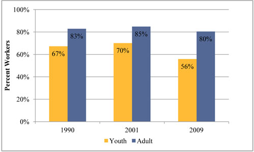
Employment trends for adults, in contrast, do not vary much over time. As Figure 28 shows, approximately 80 percent of adults identified as workers over the three time periods—a much higher proportion than youth. Across all three periods, there is about a 15-percentage point gap between working youth and adults—supporting our assertion that adult workers weather fluctuations in the economy better than youth workers.
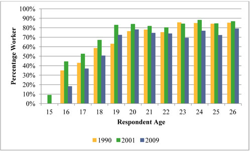
Figure 29 below shows that within the youth age group, there are stark differences in employment patterns between teens (ages 15–18) and young adults (ages 19–26). For teens, employment rates rise sharply with age in all three times periods. For young adults, employment rates do not vary much, hovering around 80 percent across all three periods. Figure 29 also shows that the proportion of working teens and adults has fallen since 2001. In fact, 2009 marks the period with the lowest proportion of working youth compared to both 1990 and 2001.
Figure 29: Percentage of Youth Working by Age and Year (1990, 2001, and 2009)
In 2009, two-thirds of working youth were non-Hispanic white (hereafter, “white”), nearly one-fifth were Hispanic, one-tenth were non-Hispanic Black (“Black”), and the remaining six percent were split evenly between NH Asian (“Asian”) and NH persons of other races (“persons of other races”). Since 1990, the proportion of Black, Asian, and persons of other races has remained steady over time. However, there have been substantial changes in unemployment rates among white and Hispanic youth (Figure 30). Since 1990, the proportion of white youth workers has decreased from over three-quarters of all working youth in 1990 to two-thirds in 2009, while the proportion of Hispanic working youth has nearly doubled from 9.5 percent in 1990 to about 18 percent in 2009—partially reflecting the increasing ethnic diversity of the nation as a whole.
Figure 30: Percentage of Working Youth by Race/Ethnicity and Year (1990, 2001, and 2009)
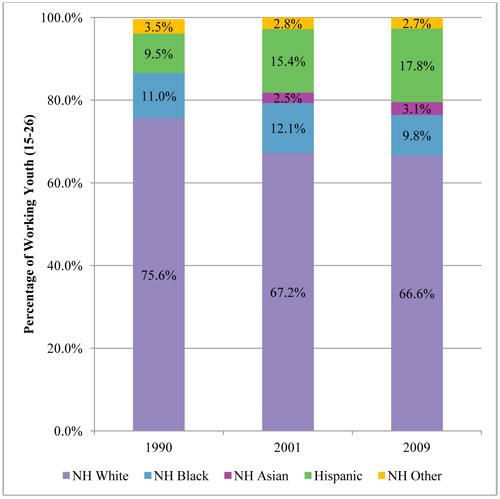
As Figure 30 shows, most of the change in the racial and ethnic composition of working youth occurred between 1990 and 2001. Despite continuing demographic shifts, youth of color have been particularly hard-hit by the recession beginning at the end of 2007 (NBER, 2008). Certainly, the proportion of youth workers overall rises and falls substantially with changes in economic conditions. As Table 30 shows, youth employment rates climbed between 1990 and the economic boom ending in 2001, and fell between 2001 and the recession starting in 2007.
As Table 30 also shows, however, there are substantial differences between employment rates within different racial and ethnic groups. In particular, employment rates are highest among white youth workers across all three years, while employment rates are lowest among Black, Asian and Hispanic youth workers. This trend reflects persistent disparities in employment rates and income among white youth and youth of color in U.S. metropolitan areas, and helps explain why the proportion of young white workers has remained relatively stable between 2001 and 2009. Interestingly, despite the major differences, it is important to note that within each racial group, employment rates have fallen at consistent rates across different racial groups (see far right column of Table 26 below).
| 1990 | 2001 | 2009 | 2009 as a % of 2001 | |
|---|---|---|---|---|
| NH White | 69.8% | 73.1% | 59.2% | 80.9% |
| NH Black | 57.7% | 61.3% | 45.8% | 74.7% |
| NH Asian | n/a | 57.6% | 46.3% | 80.4% |
| Hispanic | 63.6% | 68.0% | 53.1% | 78.1% |
| NH Other | 60.2% | 72.4% | 57.0% | 78.7% |
| Sample N | 3,200 | 6.073 | 9,539 |
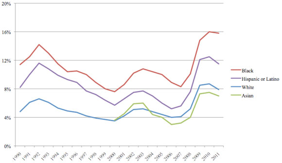
Nonetheless, the current profound economic downturn has hit communities of color the hardest. As Figure 31 below shows, the unemployment gap between white workers and Hispanic/Latino and Black workers has widened during the current recession. These differences—over time and across racial/ethnic groups—are reflected in our models of commute mode choice detailed in the next section of this chapter.
Figure 31: Unemployment by Race/Ethnicity, 1990-2011 (U.S. Department of Labor)
Commute Mode. How are people living in American metropolitan areas getting to work? Figure 32 below shows that private vehicle travel dominates commuting in U.S. metropolitan areas; across all three periods, more than 9 out of 10 workers traveled to and from their jobs by private vehicle—either alone or in a carpool. Further, despite substantial fluctuations in economic conditions, variations in real fuel prices in the midst of substantial public investments in transit systems, and the promulgation of programs to encourage carpooling, walking, and biking over the past two decades, the mode split among U.S. workers has remained remarkably stable. Bicycle commuting increased most dramatically in relative terms over the three survey periods, but by 2009 still accounted for only about one percent of all commute trips. Walking to work also increased across all three periods to nearly 4 percent in 2009—only slightly below the share of commuters carried by public transit, which fell from about 5.6 percent in 1990 to 4.6 percent in 2009.
Figure 32: Commute Mode for All Workers (1990, 2001, and 2009)
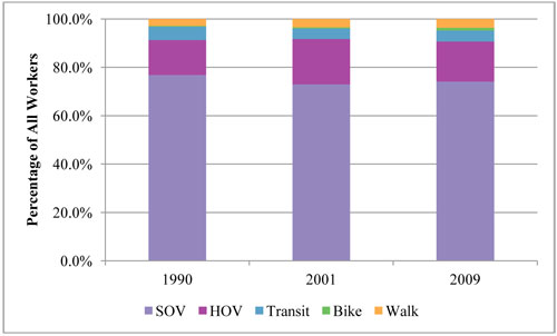
In all three periods, nearly twice as many workers carpooled to work as the combined number who biked, walked, and rode public transit. Carpooling to work increased from about 14 percent in 1990 to about 17 percent in 2001, but then dipped slightly to about 16.5 percent in 2009. Finally, and most significantly, in all three periods the vast majority of commuters—77 percent in 1990 and 74 percent in 2001 and 2009—drove alone to work.
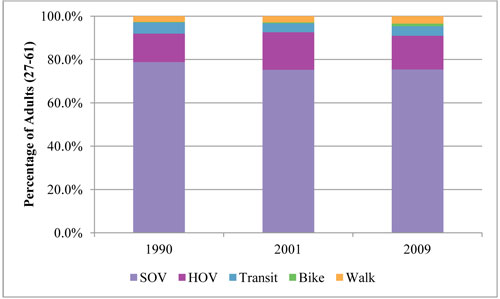
We expected that commute mode choices would differ between youth and adults, and they do—but not by much. Private vehicle commuting predominates among youth commuters, as with adults, accounting for approximately 90 percent of commute trips. Overall, travel by means other than private vehicles among youth workers is only about two percentage points higher than for adults.
Among private vehicle commuters, Figure 33 and Figure 34 show that there are much higher rates of carpooling to work among youth (nearly 23%) than that of adults (about 15%) in 2009, which has generally increased yet not changed dramatically over time. While the percentage of drive-alone commuters is much higher among adults than youth, this gap has closed slightly over time. As expected, use of non-motorized modes is higher among youth than among adults. Interestingly, however, between 2001 and 2009, we observe a decrease in bicycling among youth but an increase among adults.
Figure 33: Commute Mode for Youth (1990, 2001, and 2009)
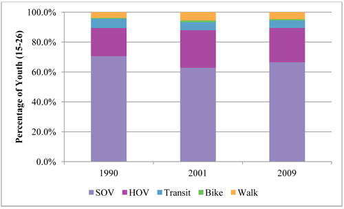
Figure 34: Commute Mode for Adults (1990, 2001, and 2009)
C. Cross-Sectional Commute Mode Model Results26
Tables 27-30 at the end of this section present our discrete choice (multinomial logistic regression) model results, which estimate the likelihood of commuting by carpool, public transit, bicycle, and walking relative to solo driving. In this section, we first explore the relationship between our variables of interest—employment, being a young adult living with parents, frequency of web use, and level of restriction of state licensing regimes—and youth commute mode choice. Then, we compare youth workers to adult workers by examining other important factors in the commute mode choice models, specifically focusing on carpooling and using transit relative to driving alone over time.
D. Variables of Interest
Young Adult Living with Parents: We find that being a young adult (ages 19-26) and living with one’s parents influences commute mode choice for youth. In 1990, holding a wide array of personal, household, trip, and geographic attributes constant, we find that young adults living with parents are more likely to drive alone to work than carpool. On the other hand, in both 2001 and 2009, young adults living with parents are more likely to take public transit to work than drive alone, all things equal.
Daily Web Use:27 We find that, for youth, using the web on a daily basis is negatively associated with choosing carpooling over driving alone to work in both 2001 and 2009. In other words, controlling for all other variables, use of the internet decreases the likelihood that a youth worker will carpool to work rather than drive alone. On the other hand, we observe a positive relationship between daily web use and commuting by transit for both youth and adults in 2001; note that we observe this effect after controlling for income. However, we see no statistically significant relationship between transit use and daily web use in 2009. We suspect this is because web use is much more common and widespread in 2009, compared to 2001, which suggests its use by a wider cross-section of society than in 2001.
Additionally, daily web use is negatively associated with commuting by bike in 2009 and positively associated with walking to work in 2001, but it is only statistically significant for adult workers.
State Licensing Regimes: Given data showing a substantial drop in driver’s licensing rates among teens in recent years, we initially hypothesized that increased strictness of a given states’ licensing regime would increase the likelihood that a teen or young adult would either carpool, ride transit or use a non-motorized form of transportation instead of driving alone to work. Indeed, state licensing regimes influence workers’ choice to commute by transit instead of driving alone, but do not appear to affect the choice to carpool. Specifically, for youth workers across all three time periods, increased strictness of licensing regimes greatly increases the likelihood that youth workers choose to commute by transit instead of driving alone—holding all things equal. The same applies to adult commuters in 1990 and 2001, but to a lesser degree.
In terms of transit use, the 2009 model shows a different trend than the other two years: while increased strictness of licensing regimes increases the likelihood of a youth worker commuting by transit, the opposite applies to adults. In particular, a youth worker living in a state with strict licensing laws is far more likely to use transit than a youth living in a state with less strict laws, while an adult worker in a more strict state is much less likely to use transit than an adult in a less strict state.
For non-motorized modes, licensing regimes have some significant but disparate effects. We find that the stricter a state’s licensing regime, the more likely adults are to bike to work in 2001 and 2009; the same goes for youth, but only in 2009. Moreover, increased strictness in licensing regimes is positively associated with walking for both youth and adults, but only in 1990. That teen driver’s licensing restrictions appear to influence adult commute mode choices raises question of whether some other factor or effect may separately influence both the likelihood of a state adopting stricter licensing rules and traveling by other modes. For example, more urbanized states may be more likely to restrict teen driving and may offer commuters of all ages more options for getting to work. Unfortunately, time and resources did not allow us to explore this question further.
E. Cross-Sectional Results by Commute Mode
Carpool: In the adult commute mode model, we find a statistically significant increase in the likelihood of carpooling among women, immigrants, and Latino workers across all three time periods—findings congruent with previous research (Blumenberg and Smart, 2010; Cline et al. 2009; Pisarski 2006; Rosenbloom and Burns, 1994). However, in our commute mode choice analysis, this only applies to adult workers; we do not observe this trend for youth workers (except for immigrant youth in 2001, who are more likely to carpool to work than their native-born counterparts are). This finding reveals some striking differences between commute patterns of youth and adult workers over all three periods.
While it is tempting to think of carpools as being comprised of two people who work at the same job site, in fact most journey-to-work carpools include people who live together (McGuckin and Srinivasan, 2005). In fact, as we mentioned in the literature review at the beginning of this report, previous research has shown that middle-aged women do far more “chauffeuring” of immediate and extended family members than do either middle-aged men or younger women, including on the commute journey (Descartes et al., 2007). Therefore, the difference we observe in carpooling between younger and older women is likely due to these differences in chauffeuring rates. As evidence of this, we find a statistically significant relationship between the number of children in the household and carpooling for all three years. For both youth and adult workers, an increase in the number of children in the household increases the odds of carpooling over driving alone to work.
Besides our finding that being a Latino adult worker increases the likelihood that one will carpool instead of drive alone to work, we find inconsistency among the effects of race/ethnicity on carpooling to work. In 1990 and 2009, Black adult workers are more likely to carpool than their white counterparts are. In 2001, the same applies to Black youth. We also find that in the 2001 model, Asian youth are less likely to carpool to work than are white youth workers. Collectively, however, these findings present no clear patterns or trends.
Other variables that influence carpooling include age, distance to work, and family income. For age, we observe that young adults are less likely to carpool to work than teens in both the 1990 and 2001 models; we observe the same trend among adults in the 2001 and 2009 models.
In terms of how commute distance influences one’s mode choice, we were surprised to observe that increased distance to work decreases the likelihood of carpooling for youth in the 2009 model and adults in the 2001 and 2009 models—contrary to previous studies’ findings (Teal, 1987; Ferguson, 1997). Though, again, these other studies that find a positive relationship between carpooling and commute distance typically focus on workers who form non-home-based carpools, in which the share of the total commute time devoted to linking up with another worker to carpool declines with longer commutes. On the other hand, research on “fampooling” has shown that significant household chauffeuring responsibilities motivates workers, particularly women, to take jobs closer to home (Schwanen et al., 2008).
Finally, in the 1990 and 2009 youth models, we find a negative correlation between household income and carpooling; working youth living in wealthier households are less likely to carpool than those living in poorer households; the same applies for adult workers in the 1990 and 2001 models.
Public Transit: Compared with other commute mode choices, geographic characteristics appear to play a much larger role in determining transit use among both youth and adults. Population density (which we measure at the Census tract level) is positively related to transit commuting for both youth and adult workers across all three periods.
Similar to previous research, we find that the denser a person’s neighborhood, the more likely that person is to commute by transit than drive alone (Crane, 2000; Pisarski, 2006; Chatman, 2009; Taylor et al., 2009). In this scenario, it is likely that both supply- and demand-side effects influence transit use. On the supply side, densely developed areas allow the same amount of transit network coverage to serve larger numbers of potential origins and destinations within a short walk of transit stops and stations. On the demand side, the number and proportion of transit users is greater in densely developed areas, because the relative costs of driving a car are greater: traffic speeds are slower, parking is more scarce and expensive, and auto insurance is more costly than in lower density areas. These two effects are mutually reinforcing, such that higher levels of transit use warrant more service, lowering headways, making transit travel speeds faster relative to driving, and thereby encouraging more transit use. Our models show that this is as true for youth as it is for adults across all three periods.
More specifically, we find that living in the New York metropolitan area—home to about 38 percent of all U.S. transit patrons—strongly increases the likelihood that workers will choose transit over solo driving. This correlation is particularly strong for youth in the 2009 model, which shows that youth living in the New York area are much more likely to commute by transit than are their counterparts in other parts of the country.
In addition to geographic characteristics, some personal and household characteristics appear to influence transit use. In particular, race/ethnicity plays a significant role in transit use. For both the youth and adult models, Black workers are far more likely to commute by transit than are white workers, after controlling for a wide variety of socio-economic factors28; this finding supports decades of research on transit usage. Further, we find that the propensity for Black workers to use transit is stronger for youth than it is for adults in the 2009 model. Indeed, the descriptive statistics are extremely suggestive: in 2009, over 25 percent of Black youth used transit to commute to work, while 13 percent of Black adults used transit. While this is still much higher than the figure for white workers (only 3 percent for both youth and adults), Black youth use transit at much higher rates than any other group in our sample.
Income also greatly influences transit use. Previous research on the topic has found that, in general, income is negatively correlated with transit use, though the relationship is weaker for commute trips than for all trips. (The sole exception to this pattern is among commuter rail users, who form a very small share of overall transit ridership and who are not separately studied here.) Consistent with previous studies, we find that income has a strong and consistent negative relationship with transit use in both the youth and adult models over all three periods. Collectively, our models suggest that income has a larger effect on youth’s use of transit than on adults.
Living in a single-family household is negatively related to transit commuting, but only for adults, who are less likely than youth to use transit than drive alone to work.
Finally, we find that having a medical condition is a significant predictor of the use of public transportation, all else being equal. Since transit includes services like paratransit, this conforms to our expectation; this is indeed the case in both the 2001 and 2009 models (the two datasets for which we have data on peoples’ medical conditions).
| Commute Mode: Carpool (base Drive Alone) | Youth 1990 |
Youth 2001 |
Youth 2009 |
Adult 1990 |
Adult 2001 |
Adult 2009 |
|---|---|---|---|---|---|---|
| Individual Characteristics | ||||||
| Age | -0.09*** |
-0.13*** |
-0.03 | 0.01 | -0.02*** |
-0.01** |
| Female | -0.08 | -0.12 | -0.16 | 0.33*** |
0.37*** |
0.44*** |
| NH White | omitted | omitted | omitted | omitted | omitted | omitted |
| NH Black | 0.17 | 0.91*** |
0.26 | 0.42*** |
0.19 | 0.46*** |
| NH Asian | no data | -2.69*** |
0.52 | no data | 0.21 | 0.36 |
| Hispanic | 0.44 | 0.19 | -0.03 | 0.49*** |
0.28** |
0.61*** |
| NH Other | -0.09 | 0.7 | 1.08* |
0.26 | 0.26 | -0.07 |
| Immigrant | no data | 0.72** |
0.17 | no data | 0.37*** |
0.23* |
| Daily Web | no data | -0.69*** |
-0.45** |
no data | -0.04 | 0.26*** |
| Medical Condition | no data | 0.6 | 1.73** |
no data | 0.83*** |
0.1 |
| Young Adult Lives with Parents | -0.46** |
0.3 | 0.24 | no data | no data | no data |
| Household Characteristics | ||||||
| Household Income (ln) | -0.34*** |
-0.11 | -0.4*** |
-0.37*** |
-0.13** |
-0.06 |
| Single Family HH | no data | -0.03 | -0.21 | no data | -0.07 | -0.02 |
| Number of Children | 0.37*** |
0.18* |
0.31*** |
0.17*** |
0.14*** |
0.16*** |
| Trip Characteristics | ||||||
| Distance to Work (log) | no data | -0.02 | -0.16* |
no data | -0.12*** |
-0.21*** |
| Peak Period Travel | no data | -0.18 | -0.08 | no data | 0.3 | -0.21* |
| Geographic Characteristics | ||||||
| Population Density (ln) | 0.10* |
-0.06 | 0.07 |
0.01 | 0.02 | -0.05 |
| New York Area | 0.28 | 0.23 | 1.02** |
0.03 | 0.19 | 0.04 |
| MSA > 3 million | 0.26 | -0.21 | -0.09 |
-0.01 | -0.13 | -0.02 |
| State Licensing Regulations | ||||||
| Stringency: Lowest | omitted | omitted | no data | omitted | omitted | no data |
| Stringency: Low | -0.15 | -0.12 | omitted | 0.05 | -0.03 | omitted |
| Stringency: Medium | no data | 0.03 | 0.17 | no data | -0.11 | -0.1 |
| Stringency: High | no data | -0.37 | 0.12 | no data | 0.03 | -0.08 |
| Constant | 3.85*** | 3.11* | 4.2*** | 1.33 | 0.24 | -0.52 |
| Sample Size | 1619 | 3006 | 3239 | 5819 | 24195 | 31721 |
| Pseudo R Squared | 0.15 | 0.27 | 0.18 | 0.11 | 0.13 | 0.14 |
| KEY: |
|---|
| Statistically Significant |
| Statistically Significant Over Time (across all the years for which data were available) |
| Commute Mode: Transit (base Drive Alone) | Youth 1990 |
Youth 2001 |
Youth 2009 |
Adult 1990 |
Adult 2001 |
Adult 2009 |
|---|---|---|---|---|---|---|
| Individual Characteristics | ||||||
| Age | -0.02 | 0.02 | -0.07 | -0.01 | -0.01 | -0.01 |
| Female | 0.41 | 0.4 | 0.17 | 0.21 | 0.23 | -0.1 |
| NH White | omitted | omitted | omitted | omitted | omitted | omitted |
| NH Black | 0.96** |
0.62 | 2.3*** |
0.82*** |
0.77*** |
0.88*** |
| NH Asian | no data | -0.56 | -0.09 | no data | 0.46 | 0.02 |
| Hispanic | -0.11 | -0.18 | -0.52 | 0.72*** |
0 | -0.36 |
| NH Other | 0.84 | 1.51** |
-1 | 1.04* |
0.33 | -0.05 |
| Immigrant | no data | 0.69 | 1.06* |
no data | -0.01 | 0.24 |
| Daily Web | no data | 0.55* |
-0.25 | no data | 0.44*** |
-0.05 |
| Medical Condition | no data | 2.43** |
1.44 | no data | 1.3*** |
1.66*** |
| Young Adult Lives with Parents | 0.48 | 1.48*** |
0.8* |
no data | no data | no data |
| Household Characteristics | ||||||
| Household Income (ln) | -0.40*** |
-0.74*** |
-0.63*** |
-0.39*** |
-0.2* |
-0.49*** |
| Single Family HH | no data | -0.39 | 0.13 | no data | -0.57*** |
-1.08*** |
| Number of Children | -0.06 | -0.07 | 0.21 | -0.24*** |
-0.05 | -0.14 |
| Trip Characteristics | ||||||
| Distance to Work (ln) | no data | -0.15 | 0.23 | no data | 0.2*** |
-0.04 |
| Peak Period Travel | no data | 2.93*** |
0.62 | no data | 0.77** |
0.26 |
| Geographic Characteristics | ||||||
| Population Density (ln) | 0.76*** |
1.03*** |
0.51*** |
0.61*** |
0.81*** |
0.64*** |
| New York Area | 0.61* |
0.28 | 2.43*** |
1.10*** |
0.96*** |
0.81*** |
| MSA > 3 million | 0.4 | 0.95** |
0.14 | -0.06 | 0.95*** |
0.71*** |
| State Licensing Regulations | ||||||
| Stringency: Lowest | omitted | omitted | no data | omitted | omitted | no data |
| Stringency: Low | 1.16*** |
1.82*** |
omitted | 0.67*** |
0.61** |
omitted |
| Stringency: Medium | no data | 1.77*** |
5.7*** |
no data | 0.4* |
-1.42* |
| Stringency: High | no data | 0.46 | 4.77*** |
no data | 0.05 | -0.82 |
| Constant | -0.06 | -0.31 | -1.8 | 0.48 | -3.43** | 3.06 |
| Sample Size | 1619 | 3006 | 3239 | 5819 | 24195 | 31721 |
| Pseudo R Squared | 0.15 | 0.27 | 0.18 | 0.11 | 0.13 | 0.14 |
| KEY: |
|---|
| Statistically Significant |
| Statistically Significant Over Time (across all the years for which data were available) |
| Commute Mode: Bicycle (base Drive Alone) | Youth 1990 |
Youth 2001 |
Youth 2009 |
Adult 1990 |
Adult 2001 |
Adult 2009 |
|---|---|---|---|---|---|---|
| Individual Characteristics | ||||||
| Age | -0.24 | -0.05 | 0.22* |
-0.04 | -0.05** |
-0.04** |
| Female | -0.95 | -1.17 | -0.82 | -1.59** |
-1.16** |
-1.85*** |
| NH White | omitted | omitted | omitted | omitted | omitted | omitted |
| NH Black | 1.62* |
-20.46*** |
-0.6 | -0.23 | -2.39** |
0.12 |
| NH Asian | no data | -4.58** |
0.18 | no data | -0.13 | -2.19*** |
| Hispanic | -22.14*** |
-1.72 | -0.35 | 0.37 | -0.89 | -1.67*** |
| NH Other | -22.16*** |
1.19 | -20.99*** |
-19.73*** |
0.2 | -1.04* |
| Immigrant | no data | 2.33*** |
0.11 | no data | 0.17 | 0.19 |
| Daily Web | no data | -1.12 | -0.45 | no data | -0.26 | -0.69* |
| Medical Condition | no data | -1.92 | -20.98*** |
no data | -2.56*** |
-0.16 |
| Young Adult Lives with Parents | 1.97* |
-0.23 | -0.48 | no data | no data | no data |
| Household Characteristics | ||||||
| Household Income (in) | -0.56 | -0.17 | 0.2 | -0.76*** |
-0.12 | -0.23 |
| Single Family HH | no data | -0.76 | -0.36 | no data | -0.06 | 0.06 |
| Number of Children | -0.05 | 0.83 | -0.08 | -0.11 | -0.53** |
0.03 |
| Trip Characteristics | ||||||
| Distance to Work (ln) | no data | -1.07*** |
-0.64*** |
no data | -0.41*** |
-0.5*** |
| Peak Period Travel | no data | 0.01 | 0.12 | no data | -0.33 | 0.15 |
| Geographic Characteristics | ||||||
| Population Density (ln) | -0.05 | 1.47*** |
0.03 | 0.48** |
0.83*** |
0.28** |
| New York Area | -0.82 | 1.78 | -0.56 | 0.31 | 1.25* |
-1.03 |
| MSA > 3 million | 0.09 | -1.73*** |
0.06 | -1.23 | -1.47*** |
0.04 |
| State Licensing Regulations | ||||||
| Stringency: Lowest | omitted | omitted | no data | omitted | omitted | no data |
| Stringency: Low | -22.78*** |
-0.61 | omitted | 0.69 | 1.96*** |
omitted |
| Stringency: Medium | no data | -1.44 | 1.81 | no data | 1.37** |
0.33 |
| Stringency: High | no data | 0.84 | 2.6** |
no data | 2.45*** |
1.21** |
| Constant | 5.58 | -2.1 | -11.29*** | 4.25 | -2.71 | 0.86 |
| Sample Size | 1619 | 3006 | 3239 | 5819 | 24195 | 31721 |
| Pseudo R Squared | 0.15 | 0.27 | 0.18 | 0.11 | 0.13 | 0.14 |
| KEY: |
|---|
| Statistically Significant |
| Statistically Significant Over Time (across all the years for which data were available) |
| Commute Mode: Walk (base Drive Alone) | Youth 1990 |
Youth 2001 |
Youth 2009 |
Adult 1990 |
Adult 2001 |
Adult 2009 |
|---|---|---|---|---|---|---|
| Individual Characteristics | ||||||
| Age | -0.13 | 0.16 | -0.01 | -0.01 | -0.01 | 0 |
| Female | 0.09 | -0.89* |
-0.86** |
0.04 | -0.08 | 0.08 |
| NH White | omitted | omitted | omitted | omitted | omitted | omitted |
| NH Black | 0 | 2.44*** |
-1.48 | -0.45 | 0.3 | 0.11 |
| NH Asian | no data | 1.73 | 0.79 | no data | -0.73 | 1.03*** |
| Hispanic | 0.09 | 0.06 | -0.21 | -0.2 | -0.2 | -0.18 |
| NH Other | -0.29 | -0.36 | -0.03 | 0.17 | -0.1 | -0.08 |
| Immigrant | no data | -0.24 | -0.15 | no data | 0.64** |
-0.29 |
| Daily Web | no data | 0.72 | 0.3 | no data | 0.77*** |
0.12 |
| Medical Condition | no data | -1.59 | 3.06*** |
no data | 0.86** |
0.19 |
| Young Adult Lives with Parents | -0.54 | -1.05 | 0.73* |
no data | no data | no data |
| Household Characteristics | ||||||
| Household Income (ln) | -0.90*** |
-0.78*** |
-0.74*** |
-0.72*** |
-0.31** |
-0.44*** |
| Single Family HH | no data | -0.68 | -1.21*** |
no data | -0.69*** |
-0.83*** |
| Number of Children | 0.21 | -0.21 | 0.24 | -0.11 | -0.16 | -0.07 |
| Trip Characteristics | ||||||
| Distance to Work (ln) | no data | -1.82*** |
-0.91*** |
no data | -0.74*** |
-0.8*** |
| Peak Period Travel | no data | 0.66 | -0.84* | no data | 0.23 | 0.1 |
| Geographic Characteristics | ||||||
| Population Density (ln) | 0.54** |
0.38* |
0.1 | 0.72*** |
0.31** |
0.31*** |
| New York Area | 0.62 | 0.97 | 1.5*** |
0.19 | 1.36*** |
0.94*** |
| MSA > 3 million | 0 | 0.33 | -0.5 | -0.03 | -0.03 | 0.01 |
| State Licensing Regulations | ||||||
| Stringency: Lowest | omitted | omitted | no data | omitted | omitted | no data |
| Stringency: Low | 0.78* |
0.64 | omitted | 1.15*** |
0.36 | omitted |
| Stringency: Medium | no data | 0.33 | -1.03 | no data | 0.34 | -0.78 |
| Stringency: High | no data | 1.12 | -1.04 | no data | 0.68 | -0.5 |
| Constant | 7.75*** | 1.17 | 8.37*** | 3.29** | 0.17 | 3.15** |
| Sample Size | 1619 | 3006 | 3239 | 5819 | 24195 | 31721 |
| Pseudo R Squared | 0.15 | 0.27 | 0.18 | 0.11 | 0.13 | 0.14 |
| KEY: |
|---|
| Statistically Significant |
| Statistically Significant Over Time (across all the years for which data were available) |
F. Quasi-Cohort Model Results
Table 35 shows the results of a quasi-cohort model of commute mode choice in which we estimate the probability of driving alone to work rather than using any other mode of transportation. The coefficients on the control variables carry their expected signs and broadly conform to the findings from our cross-sectional analyses. The model suggests that women and all non-white racial and ethnic groups are less likely to drive alone than are men and whites. Education, income, and greater access to automobiles are all positively associated with driving alone to work, all else equal. The model also suggests that those living in denser and larger urban areas, as well as those commuting on the weekend, are less likely to drive alone.
| Coefficient | Sig. | t-Statistic | p-value | |||
|---|---|---|---|---|---|---|
| Individual Characteristics | ||||||
| Female | -0.064 | *** | -3.42 | 0.001 | ||
| Age | 0.247 | *** | 25.52 | <0.001 | ||
| Age Squared | -0.003 | *** | -24.59 | <0.001 | ||
| Race / Ethnicity (omitted category: Non-Hispanic White) | ||||||
| Non-Hispanic Black | -0.290 | *** | -7.94 | <0.001 | ||
| Non-Hispanic Asian (2009 Only) | -0.114 | ** | -2.21 | 0.027 | ||
| Non-Hispanic Other | -0.221 | *** | -3.9 | <0.001 | ||
| Hispanic | -0.034 | -1 | 0.319 | |||
| Uses Web Daily | 0.128 | *** | 5.67 | <0.001 | ||
| Education (omitted category: No HS Diploma) | ||||||
| For Youth: Highest Degree Achieved in Household | ||||||
| High School Diploma | 0.659 | *** | 8.12 | <0.001 | ||
| Some College | 0.785 | *** | 10.21 | <0.001 | ||
| Bachelor's Degree | 0.799 | *** | 10.01 | <0.001 | ||
| Graduate Degree | 0.557 | *** | 6.25 | <0.001 | ||
| For Adults: Highest Degree Personally Achieved | ||||||
| High School Diploma | 0.426 | *** | 7.29 | <0.001 | ||
| Some College | 0.593 | *** | 10.19 | <0.001 | ||
| Bachelor's Degree | 0.534 | *** | 8.94 | <0.001 | ||
| Graduate Degree | 0.415 | *** | 6.75 | <0.001 | ||
| Household Characteristics | ||||||
| Income (ln) | 0.111 | *** | 8.19 | <0.001 | ||
| Number of Adults in HH | 0.023 | * | 1.92 | 0.055 | ||
| Number of Children in HH | -0.127 | *** | -14.54 | <0.001 | ||
| Youth, Lives with Parents | 0.715 | *** | 14.02 | <0.001 | ||
| Ratio of Cars to Adults in HH | 1.381 | *** | 50.28 | <0.001 | ||
| Geographic Characteristics | ||||||
| Population Density (ln) | -0.115 | *** | -17.68 | <0.001 | ||
| In MSA with > 3M Population | -0.261 | *** | -12.62 | <0.001 | ||
| Weekend | -0.376 | *** | -13.27 | <0.001 | ||
| Year | ||||||
| Year: 2001 (base: 1990) | -0.505 | *** | -10.65 | <0.001 | ||
| Year: 2009 (base: 1990) | -0.653 | *** | -9.83 | <0.001 | ||
| Cohorts (base: Born before 1950) | ||||||
| Born in 1950s | -0.003 | -0.06 | 0.950 | |||
| Born in 1960s | 0.075 | 1.06 | 0.288 | |||
| Born in 1970s | 0.524 | *** | 5.37 | <0.001 | ||
| Born in 1980s | 0.370 | *** | 2.93 | 0.003 | ||
| Born in 1990s | 0.277 | * | 1.77 | 0.077 | ||
| Constant | -6.309 | -22.92 | <0.001 | |||
| N | 98,276 | |||||
| R-Square | 0.126 | |||||
Turning now to our variables of interest, we find that youth living with their parents are considerably more likely to drive alone to work, as are those who use the web daily. Over time, the model suggests a decreasing trend in single-occupant auto commutes, controlling for other variables included in the model. This finding seemingly contradicts the descriptive statistics, which show a rapid increase in drive-alone commutes during the 1990s, and a slower increase from 2001 to 2009. The model’s suggestion of a negative independent effect of the 2001 and 2009 data years may suggest that the observed increase in SOV commutes are explained by other variables in the model, such as auto ownership, which also increased rapidly during our study period.
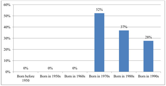
Finally, the cohort variables suggest that newer cohorts have an increased likelihood of driving alone to work than previous cohorts, but that this effect is diminishing over time. As Figure 35 indicates, the model finds that those born in the 1970s are 52 percent more likely to choose to drive alone to work than are those born before 1950, all else equal. Those born in the 1980s and 1990s have a similarly elevated but diminishing probability of driving alone, with a 37 percent and 28 percent increase in the likelihood of driving alone, ceteris paribus.
Figure 35: SOV Independent Effect of Cohort, Controlling for Other Variables
G. Conclusion: Commute Mode Findings
While the previous two analyses found that working has a substantial influence on both personal miles traveled and the number of daily trips, this analysis has focused specifically on the mode choices of workers. As with the previous analyses, the effects of the recession on travel behavior, particularly by youth, are substantial. While the proportion of working adults declined from 85 to 80 percent between 2001 and 2009, the number of working youth dropped precipitously, from 70 percent in 2001 to just 56 percent in 2009.
While the proportion of adult and, especially, young workers was much lower in 2009 than in 2001, the analysis in this chapter focused on how those who do work get there. We find, not surprisingly, that household income is a consistent predictor of commute mode choice for both youth and adults. In general, income is strongly and positively associated with driving alone to work; put another way, as incomes go up, the probability of commuting via carpool, public transit, bicycle, or foot all go down—for both youth and adults, and across all three survey years.
With respect to the effect of the bad economy causing a growing number of youth to “boomerang” home to live with parents, we find that young working adults living at home are less likely to carpool and more likely to use public transit than other workers. Likewise, those who use the web daily were less likely to carpool (2001 and 2009) and more likely to commute via public transit (2001 only). Last, in terms of our variables of interest, youth in places with stricter teen licensing regimes were more likely to commute to work via public transit; however, we find that the strictness of licensing regimes has no significant effect on an individual’s choice to commute via carpool.
The analysis also revealed important differences between youth and adult workers. Previous studies have consistently shown that being female, Hispanic, or foreign born increases the likelihood of commuting by carpool over driving alone. Our analysis shows that trend remains consistently strong for adults, but not for young workers. This suggests that the relationship between travel mode broad social categories, like sex, race/ethnicity, and immigration status, may be weakening over time.
Finally, the quasi-cohort model suggests that those born in more recent decades (the 1970s, 80s, and 90s) are far more reliant on the single-occupancy vehicle for their journey to work than were previous generations, though this effect appears to be diminishing over time.
| Youth (15–26) 1990 |
Youth (15–26) 2001 |
Youth (15–26) 2009 |
Adult (27–61) 1990 |
Adult (27–61) 2001 |
Adult (27–61) 2009 |
|
|---|---|---|---|---|---|---|
| Commute Mode | ||||||
| Model N | 1,619 | 3,006 | 3,239 | 5,819 | 24195 | 31721 |
| Pseudo R2 | 0.15 | 0.27 | 0.18 | 0.11 | 0.13 | 0.14 |
| Youth (15–26) 1990 |
Youth (15–26) 2001 |
Youth (15–26) 2009 |
Adults (27–61) 1990 |
Adults (27–61) 2001 |
Adults (27–61) 2009 |
|
|---|---|---|---|---|---|---|
| HOV (Base: driving alone) | ||||||
| Employment Status | (Not included in the model) | (Not included in the model) | ||||
| Young Adult Living at Home | - |
0 |
0 |
n/a | n/a | n/a |
| Technology (Web Use) | n/a | - |
- |
n/a | 0 |
+ |
| License Stringency | 0 |
0 |
0 |
0 |
0 |
0 |
Transit (Base: driving alone) | ||||||
| Employment Status | (Not included in the model) | (Not included in the model) | ||||
| Young Adult Living at Home | 0 |
+ |
+ |
n/a | n/a | n/a |
| Technology (Web Use) | n/a | + |
0 |
n/a | + |
0 |
| License Stringency | + |
+ |
+ |
+ |
+ |
- |
Bicycling (Base: driving alone) | ||||||
| Employment Status | (Not included in the model) | (Not included in the model) | ||||
| Young Adult Living at Home | + |
0 |
0 |
n/a | n/a | n/a |
| Technology (Web Use) | n/a | 0 |
0 |
n/a | 0 |
- |
| License Stringency | - |
0 |
+ |
0 |
+ |
+ |
Walking (Base: driving alone) | ||||||
| Employment Status | (Not included in the model) | (Not included in the model) | ||||
| Young Adult Living at Home | 0 |
0 |
+ |
n/a | n/a | n/a |
| Technology (Web Use) | n/a | 0 |
0 |
n/a | + |
0 |
| License Stringency | + |
0 |
0 |
+ |
0 |
0 |
25For our commute mode analysis over time, we derive our sample from those who reported a commute mode—which is a smaller pool than all workers in this table—resulting in sample sizes of 7,438 youth and adult workers in 1990, 16,195 in 2001, and 35,003 in 2009.
26Unless otherwise noted, all results that we discuss in this section are statistically significant at the .01 (denoted by “***”), .05(“**”), or .10(“*”) levels.
27As noted above, there is no daily web use for 1990, so compare web use between 2001 and 2009.
28This finding is statistically significant in all but the 2001 youth model.