U.S. Department of Transportation
Federal Highway Administration
1200 New Jersey Avenue, SE
Washington, DC 20590
202-366-4000
Federal Highway Administration Research and Technology
Coordinating, Developing, and Delivering Highway Transportation Innovations
 |
| This report is an archived publication and may contain dated technical, contact, and link information |
|
Publication Number:
FHWA-RD-03-048
|
Previous | Table of Contents | Next
The purpose of the current study is to investigate the behavior of MSEWs with modular block facing and geosynthetic reinforcement using the two-dimensional finite difference program FLAC (Version 3.40, Itasca 1998). A set of computer runs identified failure mechanisms of MSEWs as function of geosynthetic spacing, considering the effects of soil strength, reinforcement stiffness, connection strength, secondary reinforcement layers, and foundation stiffness. Numerical analysis also was conducted to investigate the effects of reinforcement length on reinforcement stresses and wall stability. FLAC predictions were compared with the existing design method (AASHTO 98) using the MSEW 1.1 program (ADAMA Engineering 1998). Additional numerical experiments investigated the effect of some modeling parameters on the predicted wall response.
The behavior of MSEW with modular block facing and geosynthetic reinforcement was investigated with numerical models that simulate construction of the wall, layer by layer, until it fails under gravity loading. Various responses during wall construction such as displacement accumulation, stress histories, and tensile load in reinforcement, can be recorded. The components and basic geometry of the model are shown in figure 3.1.
The numerical model is updated continuously by adding soil and geosynthetic layers up to failure in stages, which represent the construction sequence of actual walls. The first reinforcement layer is always installed at elevation 0.2 m on top of the first soil layer and the first block. Next, reinforcement layers are installed according to the reinforcement spacing. For example, the modeling sequence of a wall with reinforcement spacing equal to 0.4 m consists of the following stages (figure 3.2):
Wall construction continues up to failure following the same pattern.
The construction using the numerical model continues until the program stops due to excessive deformations in a certain element (bad geometry). At this stage, the deformations in the system were large and corresponded essentially to a failed wall. Numerical and physical parameters such as slip surface development, maximum displacement of the system accumulated during wall construction, number of calculation steps necessary to equilibrate the system after placement of each layer, and history of maximum unbalanced force, allowed (Who? What?) to define a critical wall height. This height corresponds to a wall at the verge of failure (figure 3.3–b). All states corresponding to a height larger than the critical one are considered as failure states (figure 3.3–a). To investigate the effects of reinforcement length on wall stability, the wall height of certain numerical tests was kept equal to the critical one, while the length of reinforcement was increased. For these tests, the states that correspond to walls with length-to-height ratio larger than the critical one are considered as stable states (figure 3.3–c).
The major components of the model are foundation, modular blocks, reinforced soil, retained soil (backfill), and reinforcements layers (figure 3.1). A set of model variables (listed in table 3.1) was implemented to allow change of geometry and material properties according to the purpose of the analysis.
A typical numerical grid and dimensions to discretize the problem are shown in figure 3.4. The wall and the adjacent backfill with uniform grid density form a 'kernel' of the numerical model. Its dimensions can be changed accordingly (zones 1 and 2 in figure 3.5). The grid around that kernel models the foundation soil and the end part of the backfill adjacent to model boundaries (zones 3 to 6 in figure 3.5). The foundation depth and width of end backfill were fixed to 5.0 m for all simulations.
Grid density of the model is shown on figure 3.5. The grid in zone 1 (figure 3.5–a) represents the wall facing constructed from separate modular blocks. The block-block, block-soil, and block-reinforcement interaction is modeled interfacing with properties that can be changed accordingly. In the final version of the model, the modular blocks are divided into rectangular elements with dimensions 0.05 x 0.1 m (uniform density in both directions of zone 1) (figure 3.5–b). In early parametric studies, the modular blocks were represented either by one element or divided into square elements with dimensions 0.1 x 0.1 m (figure 3.5–c); however, to represent the interaction at the connections more accurately, numerical sensitivity analysis indicated that horizontal grid density should be increased. Zone 2 consists of 2 parts (figure 3.5–a). Part 2–a corresponds to the reinforced soil, and part 2–b corresponds to a part of the retained soil adjacent to the reinforced soil. Both parts of zone 2 can change their global horizontal dimension by changing the model variables "length of reinforcement, /l" (zone 2–a) or "length of adjacent backfill, /L" (table 3.1). The grid density of zone 2 is uniform in both directions and can be changed by changing the model variable "number of sublayers within a height of 0.2 m (fixed height of a modular block), /nsl" (table 3.1). In the final version of the model, the elements of zone 2 are squares with dimensions /a x /a m, where /a is defined as follows:
However, in the current analysis, the influence of grid density in zone 2 less than 0.1 x 0.1 m resulted in numerical instability. Numerical tests were done with grid density in zone 2 corresponding to element size 0.05 x 0.05 m and numerical instability constantly occurred at a wall height of about 2 m. Because of the encountered numerical instability at such small dimensions, the grid density in zone 2 was kept constant, corresponding to the smallest stable element size of 0.1 x 0.1 m. In zone 3 (end part of the backfill), grid density is uniform vertically and changes gradually in horizontal direction. The element size changes from left to right from 0.1 x 0.1 m to 0.5 x 0.1 m. In zone 5 (middle part of foundation), grid density is uniform in horizontal direction and changes gradually in vertical direction. The element size changes from top to bottom from 0.1 x 0.1 m to 0.1 x 0.5 m. In zones 4 and 6 (left and right parts of the foundation), grid density changes gradually in both directions. The element size changes from 0.1 x 0.1 m to 0.5 x 0.5 m. Grid density of the model was defined with respect to the modular block height (hbl= 0.2 m), with ability to be changed within the zone 2 (figure 3.5). In all numerical tests, the smallest stable element size was used? 0.05 x 0.1 m in zone 1 (facing) and 0.1 x 0.1 m in the soil. Figure 3.4 shows a typical grid in all zones.
Boundary conditions of the model consist of prescribed zero velocities (corresponding to zero displacements) perpendicular to the boundaries (figure 3.5). Boundary effects on model response were investigated with respect to the distance of the wall to the right model boundary. In the final version of the model, the total width of backfill is 15.0 m (the width of zone 2–b is 10.0 m, and the width of zone 3 is 5.0 m, figure 3.5). For all numerical simulations, this backfill width ensured that the deformed zone behind the wall was not close to the model boundary. Several numerical simulations varied the width of backfill from 5.2 m to 15.0 m (/L=0.2–10.0 m). It was proved that boundary affected the results significantly when the active zone that developed behind the wall was close to or reached the right model boundary. Close boundary effects increased wall stability because of the restraint horizontal displacements along the right model boundary. To avoid boundary effects on model response, additional tests were done for a model (case 1, s=0.2 m, h=6.6 m, /l=1.5 m), varying the width /L of the adjacent backfill (zone 2–b on figure 3.5). The distributions of stresses and horizontal displacements along a vertical section 0.1 m behind the facing are shown on figure 3.7 for /L=6, 8 and 10 m. The differences were less than 5 percent. In all consequent numerical tests, the width of the backfill was 15.0 m (/L=10 m).
Wall facing was specified as concrete modular blocks with a fixed height of 0.2 m and a fixed thickness of 0.2 m. Each new block was placed precisely on top of the previous one. As construction progressed, the facing tilted outward as a result of cumulative displacements. Block-block, block-reinforcement, and block-soil interaction was modeled with interfaces along which sliding or separation can occur.
During construction, reinforcement layers were placed, following the scheme set by the specified spacing (figures 3.2 and 3.8). Each reinforcement layer was designed with two parts, using beam and cable structural elements available in FLAC. The reinforcement section confined between the facing blocks was modeled using a FLAC beam element. The reinforcement section embedded in soil was modeled using a FLAC cable element. The beam and cable elements were linked at a common node. FLAC beam elements are two-dimensional elements with three degrees of freedom at each end node (x-translation, y-translation and rotation). These elements represent structural members in which bending resistance is important. Beam elements can be joined together with each other and the grid, directly or through interface elements. FLAC cable elements are one-dimensional axial elements that may be anchored at a specific point in the grid or grouted so that the cable elements develop forces along its length as the grid deforms. They cannot sustain bending moments and are used to model supports for which tensile capacity is important. Cable elements interact with the confining material only when they are grouted. To represent the frictional connection between the modular blocks and the reinforcement correctly, the reinforcement was modeled in two parts using beam and cable elements. Beam elements represent the block-reinforcement interaction. Because beam elements can interact with the grid only through interfaces or explicitly specified links, they were not used to model the reinforcement-soil interaction. Cable elements were used to represent the soil-reinforcement interaction, because they cannot be used with the interfaces that model the block-reinforcement interaction.
Each wall was modeled to reach failure by increasing its height in layers while keeping the reinforcement length equal to 1.5 m. In the process of numerical simulation, the wall reached the verge of failure, but its construction continued until the failure was detected numerically. The state that corresponds to a wall at the verge of failure was called a critical state. A critical state is defined by analyzing numerical and physical parameters such as slip surface development, number of calculation steps necessary to equilibrate the system after placement of each layer (figures 3.9–a, 3.10–a, 3.11–a) maximum cumulative displacement of the system during construction (figures 3.9–b, 310–b, 3.11–b), and history of maximum unbalanced force. In the current studies, a critical state was identified when at least three of the following events occurred simultaneously: (1) a slip surface was developed fully, (2) the maximum cumulative displacement increases nonlinearly, (3) the number of calculation steps per layer increased rapidly, and (4) the history of maximum unbalanced force indicated an abrupt change of the unbalanced force. Figures 3.9– 3.11 provide typical plots showing the maximum cumulative displacements and the number of calculation steps (necessary to equilibrate the system after the placement of each layer) .
The height and length-to-height ratio at the critical state are called critical height (hcr) and critical length-to-height ratio (/l/hcr), respectively. States of a model that correspond to walls higher than the wall at the critical state are called failure states. Stable states correspond to walls with a height equal to the critical height and a length-to-height ratio larger than the critical length-to-height ratio. The definition of failure, critical, and stable states of a numerical model is illustrated on figure 3.3.
In the process of numerical simulation, the wall is constructed until the failure is detected numerically (i.e., the model construction stops). The model stops in the following two cases:
The equilibrium state in FLAC is identified when one of the following happens: (1) the number of calculation steps reaches the specified limit (default value is 100,000); or (2) the largest ratio of maximum unbalanced force2 to average applied force is below a specified limit called "equilibrium ratio" (default value is 0.001). Computer runs investigated the influence of these model response limits. Typical results are presented on figures 3.9–3.11, and in table 3.2. The presented results proved that the model response is not influenced when the equilibrium ratio was changed from 0.001 (default value) to 0.01, and when the maximum number of steps was changed from 100,000 (default value) to 200,000. In all numerical simulations, the equilibrium ratio was /srat=0.01 (10 times larger than the default value), and the maximum number of calculation steps was 100,000 (default value).
The material properties used in the analysis were based on data reported in the literature. They represent typical values used in design practice (Das 1999).
The soil was modeled as a cohesionless material using a FLAC plastic constitutive model that corresponds to a Mohr-Coulomb failure criterion with a hyperbolic stress-strain relationship. The elastic modulus of soil was updated after placement and equilibration of each soil layer using the following hyperbolic stress- strain relationship (Wong and Duncan 1974):

where: Es = elastic modulus of soil; Pa = atmospheric pressure; σ3 = minor principal effective stress; and K and /m are the hyperbolic model coefficients. For all numerical simulations, the hyperbolic model coefficient /m was kept constant equal to 0.5 (Bathurst and Hatami 1999, Ling et al. 2000). The soil properties were changed to investigate different aspects of wall behavior. The soil properties that were used in different numerical tests are summarized in tables 3.3 and 3.4.
1 Because FLAC is an explicit code, the solution to a problem requires a number of computational steps. During computational stepping, the information associated with the phenomenon under investigation is propagated across the zones in the finite difference grid. A certain number of steps is required to arrive at an equilibrium or steady flow state for a static solution (FLAC User's Guide, Itasca 1998).
2 The unbalanced force indicates when a mechanical equilibrium state (or the onset of plastic flow) is reached for a static analysis. A model is in exact equilibrium if the net nodal force vector at each gridpoint is zero. The maximum nodal force vector is monitored in FLAC (called the unbalanced force) and will never reach exactly zero for a numerical analysis. The model is considered to be in equilibrium when the maximum unbalanced force is small compared to the total applied forces in the problem (FLAC User's Guide, Itasca 1998).
The modular blocks were modeled using a linear elastic constitutive model. The geometry, parameters, and properties of the facing were kept constant for all numerical runs and are given in table 3.5.
The reinforcement layers were modeled using beam and cable structural elements available in FLAC. The properties of the cable and beam elements used in different numerical tests are summarized in table 3.6.
The block-block, block-reinforcement, and block-soil interaction was modeled using interfaces available in FLAC. Three types of interfaces were used in the model: between two facing blocks (block-block interface), between a facing block and the part of reinforcement modeled by a beam element (block-beam interface or block-reinforcement interface), and between a facing block and the adjacent soil (block-soil interface). The interfaces are sketched in figure 3.8. They represent planes along which sliding or separation can occur and are characterized by the Coulomb shear-strength criterion:
where: /Fsmax = maximum shear force, /c = cohesion along the interface, /Le = effective contact length, Fn = normal force, and δ = friction angle of interface surfaces. If shear forces in interfaces are less than the maximum shear strength defined by Equation (3.3), sliding or separation occurs.
The properties of block-block and block-reinforcement interfaces were changed to simulate different connection strengths between the reinforcement and the modular blocks. Frictional connection was represented by interfaces with no cohesion, and the interface angle of friction was changed to investigate its influence on wall behavior. Structural connection was represented by interfaces characterized with both cohesion and friction. Block-soil interfaces were always modeled with no cohesion. Interface properties used in analysis are summarized in table 3.7. To ensure numerical stability, the normal and shear stiffness of the interfaces were modeled following the guidelines given in the FLAC manual (Itasca 1998). The normal stiffness of interfaces was assigned to correspond to the bulk modulus of concrete. The shear stiffness of interfaces was assigned to correspond to the initial shear modulus of reinforced soil.
The interaction between reinforcement layers and soil is represented by grout-soil interface defined as a part of the cable element definition. Properties of grout as part of the cable elements definition are given in table 3.6.
Parametric studies investigated the behavior of MSEWs with modular block facing and geosynthetic reinforcement using a numerical model that can simulate construction sequence layer by layer up to failure. A set of runs identified failure mechanisms of MSEWs as function of geosynthetic spacing, considering the effects of soil strength, reinforcement stiffness, connection strength, use of secondary reinforcement layers, and foundation. A second set of numerical runs investigated the effects of reinforcement length on reinforcement stresses and wall stability. FLAC predictions were compared with an existing design method (AASHTO 98) using the MSEW 1.1 program (ADAMA Engineering 1998). Additional numerical runs investigated the effect of some model parameters on the predicted wall response. All numerical runs were grouped into cases according to the set of properties used in the analysis. Within each case, numerical runs with different reinforcement spacing were performed. Summary of all parametric studies is given in table 3.8.
Cases 1, 2, and 3 represent models with very stiff foundation and soil strength of reinforced and retained soil decreasing from case 1 (high strength soil) to case 3 (low strength soil). Cases 4, 5, and 6 represent models with soil properties that are the same for the entire model, with soil strength decreasing from case 4 (high strength soil) to case 6 (low strength soil). For cases 1 to 6, the connection between the reinforcement and facing is frictional (baseline strength, table 3.7), and reinforcement properties correspond to typical design values (baseline reinforcement (BR), table 3.6). All relevant reinforcement spacings within the range of 0.2 to 1.0 m were investigated.
Cases 7 to 12 were designed to investigate certain aspects of wall behavior complementing the first six cases. Case 7 was designed to assess the effects of secondary reinforcement layers (figure 3.12). Model properties of case 7 were the same as the model properties of case 2,with the exception of reinforcement layout, which consists of primary reinforcement layers at every 0.6 m (/l=1.5 m) and secondary reinforcement layers in between at every 0.2 m (/l=0.3 m). Cases 8–1, 8–2, and 8–3 were designed to investigate the effects of reducing the reinforcement stiffness on wall response. The effect of connection strength was investigated with cases 9 (low strength frictional connection) and case 12 (structural connection). Case 10 was designed to investigate the wall behavior considering weak foundation. Case 11 was designed to investigate the effect of soil dilatancy on wall behavior.
Additional runs were carried out to investigate the effect of grid density, boundary distance (i.e., boundary effects), and values of FLAC equilibrium limits.
Four numerical models corresponding to different failure mechanisms were investigated with respect to failure and stable states, and are called baseline cases. The set of numerical experiments for case 1 and some of the corresponding modified cases is represented with an organizational chart in figure 3.13.
Thirty-seven runs were directly involved in the analysis (table 3.8). The runs were performed on three personal computers. One of the runs was completed with an Intel® x86 Processor, 384 MB RAM, 800 MHz; the other two runs were completed with Pentium® II Processor Intel MMXTM, 128 MB RAM, 550 MHz. The total time of these 37 runs was about 900 hours, or 106 working days. General information about the runs of all cases (at failure and critical states) is given in table 3.9 and table 3.10. Typical input file is given in the appendix.
Figure 3.1 Numerical Model Components.
Figure 3.2 Schematic of Modeling of Construction Sequence of Wall with Reinforcement Spacing Equal to 0.4 m.
Figure 3.3 Definition of: (a) Failure State; (b) Critical State; (c) Stable State.
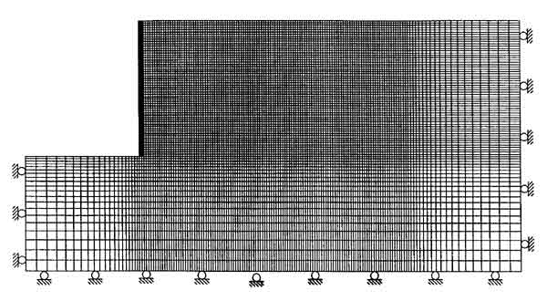
Figure 3.4 Typical Numerical Grid
Figure 3.5 Grid Definition: (a) Model Zones with Respect to Grid Generation; (b) Grid of Modular Blocks in the Current Model; (c) Grid of Modular Blocks in Early Versions of the Model.
NOTE: L=Width of adjacent backfill grid (figure 3.5).
Figure 3.6 Boundary Effects on Model Response: Horizontal Displacements along Vertical Section A Located 0.1 m behind the Facing.
NOTE: L=Width of adjacent backfill (zone 2–a, figure 3.5).
Figure 3.7 Boundary Effects on Model Response: Stress Distributions along Vertical Section A Located 0.15 m behind the Facing.
Figure 3.8 Types of Interfaces at the Blocks.
Figure 3.9 Baseline Cases: (a) Number of Calculation Steps Necessary to Equilibrate Each Layer; (b) Maximum Cumulative Displacement during Wall Construction.
Figure 3.10 Effects of FLAC Equilibrium Ratio Limit on Model Response of Case 1 (s=0.2 m, l=1.5 m): (a) Number of Calculation Steps; (b) Maximum Cumulative Displacement.
Figure 3.11 Effects of FLAC Step Limit on Model Response of Case 12 (s=0.2 m, l=1.5 m): (a) Number of Calculation Steps; (b) Maximum Cumulative Displacement.
Figure 3.12 Reinforcement Layout with Primary and Secondary Layers for Case 7 (s=0.6/0.2 m).
Figure 3.13 Some of the Executed Numerical Runs.
| Model Variable | Notation | Comment | |
|---|---|---|---|
| Wall dimensions and grid density | Wall height | h | Multiple of 0.2 m |
| Length-to-height ratio | /l/h | Must correspond to wall height multiple of 0.2 m | |
| Length of reinforcement | l | Multiple of 0.1 m | |
| Length of adjacent backfill | L | Multiple of 0.1 m | |
| Number of blocks between two reinforcement layers | nbl | Defines the reinforcement spacing. For example, if nbl=4, the corresponding reinforcement spacing is s=nbl*0.2=0.8 m (0.2 m is a fixed height of a modular block) | |
| Number of sublayers within a height of 0.2 m | nsl | Defines grid density in reinforced soil and the adjacent backfill | |
| Soil | Friction angle | Different values for soil in foundation, wall and backfill can be specified | |
| Poisson's ratio | /vs | ||
| Initial elastic modulus | Eis | ||
| Facingblocks | Elastic modulus | Eib | It is recommended that this value does not exceed the elastic modulus of soil more than 10 times (Itasca 1998) |
| Poisson's ratio | /vb | – | |
| Reinforcement | Cable elastic modulus | Ec | – |
| Grout shear stiffness | kbond | – | |
| Grout cohesive strength | sbond | – | |
| Beam elastic modulus | Eb | – | |
| Interfaces | Normal stiffness | kn | If these values are not derived from tests on real joints, it is recommended that they are less than ten times the equivalent stiffness of interacting materials (Itasca 1998) |
| FLAC Equilibrium Ratio Limit | Number of Steps | Maximum Displacement (cm) | Maximum Axial Force | Maximum Connection Force | ||
|---|---|---|---|---|---|---|
| Value (kN) | at Elevation (m) | Value (kN) | at Elevation (m) | |||
| 0.01 | 419538 | 4.4 | 6.02 | 1.2 | 4.83 | 1.2 |
| 0.001 | 882890 | 4.38 | 6.04 | 0.8 | 4.58 | 0.8 |
| Parameter | Soil Type | Comments | ||
|---|---|---|---|---|
| High Strength Soil (HS) | Medium Strength Soil (MS) | Low Strength Soil (LS) | ||
| Friction angle (deg) | 45 | 35 | 25 | Model variable |
| Dilation angle (deg) | 15 | 7 | 0 | – |
| Cohesion (kPa) | 0 | 0 | 0 | – |
| Initial modulus of elasticity (MPa) | 60 | 60 | 60 | Model variable |
| Poisson's ratio | 0.3 | 0.3 | 0.3 | Model variable |
| Density (kg/m3) | 2200 | 2200 | 2200 | – |
| Parameter | Soil Type | Comments | ||
|---|---|---|---|---|
| Baseline Stiff Soil (BSt) | Very Stiff Soil (VSt) | |||
| Initial modulus of elasticity (MPa) | 60 | 60 | Model variable | |
| Stress-strain relationship | Hyperbolic constitutive model | Hyperbolic constitutive model | See equation (3.2) | |
| Hyperbolic model parameters: | K | 270.2 | 270200 | (Ling et al. 2000) |
| m | 0.5 | 0.5 | ||
| Cohesion (kPa) | 0 | 1000 | – | |
| Parameter | Value | Comments |
|---|---|---|
| Height (m) | 0.2 | Fixed |
| Thickness (m) | 0.2 | Fixed |
| Density (kg/m3) | 2200 | Corresponds to dry cast concrete |
| Elastic modulus (MPa) | 600 | Model variable; ten times larger than initial elastic modulus of soil; linear elastic stress-strain relationship used |
| Poisson's ratio | 0.15 | Model variable |
| FLAC Modeling Element | Parameter | Reinforcement Type | Comments | |
|---|---|---|---|---|
| Baseline Reinforcement (BR) | Ductile Reinforcement (DR) | |||
| Cable | Area (m2) | 0.002 | 0.002 | Corresponds to rectangular cross section 0.002x1.0 m |
| Perimeter (m) | 2.0 | 2.0 | – | |
| Cable elastic modulus (kN/m2/m) | 106 (EA=2000 kN/m) | 105 (EA=200 kN/m) | Model variable | |
| Cable tensile yield strength (kN/m) | 200 | 200 | – | |
| Grout shear stiffness (kPa) | 23077 (Equal to Initial Shear Modulus of Soil) | 2307.7 (Equal to 1/10 of Initial Shear Modulus of Soil) | Model variable, characterizes soil- reinforcement interaction | |
| Grout cohesive strength (kN/m) | 100 | 100 | Model variable, characterizes soil- reinforcement interaction | |
| Grout frictional resistance (deg) | 35 | 35 | Characterizes soil- reinforcement interaction | |
| Beam | Area (m2) | 0.002 | 0.002 | – |
| Elastic modulus (MPa) | 1000 | 100 | Model variable | |
| Moment of inertia (m4) | 6.67x10⁻¹⁰ | 6.67x10⁻¹⁰ | Corresponds to cross section 0.002x1.0 m | |
| Parameter | Connection Type | Comments | ||
|---|---|---|---|---|
| Frictional Connection: Low Strength (FCon–L) | Frictional Connection: Baseline Strength (FCon–N) | Structural Connection (SCon) | ||
| Interface friction angle (deg) | 20 | 30 | 30 | – |
| Interface cohesion (kPa) | 0 | 0 | 20 | – |
| Interface normal stiffness (kPa/m) | 285714 | 285714 | 285714 | Model variable, corresponds to bulk modulus of concrete blocks |
| Interface shear stiffness (kPa/m) | 23077 | 23077 | 23077 | Model variable, corresponds to initial shear modulus of soil |
| Case | Spacing (m) | Soil Type in | Reinforcement Type | Connection Type | Comments | ||
|---|---|---|---|---|---|---|---|
| Foundation | Backfill | Wall | |||||
| 1 | 0.2
0.4
0.6
0.8
1.0 |
HS
VSt |
HS
BSt |
HS
BSt |
BR | FCon–B | Baseline case, s=0.2 m |
| 2 | 0.2
0.4
0.6
0.8 |
MS
VSt |
MS
BSt |
MS
BSt |
BR | FCon–B | Baseline case, s=0.6 m |
| 3 | 0.2
0.4
0.6
0.8 |
LS
VSt |
LS
BSt |
LS
BSt |
BR | FCon–B | – |
| 4 | 0.2
0.4
0.6
0.8 |
HS
BSt |
HS
BSt |
HS
BSt |
BR | FCon–B | – |
| 5 | 0.2
0.4
0.6
0.8 |
MS
VSt |
MS
BSt |
MS
BSt |
BR | FCon–B | – |
| 6 | 0.2
0.4 |
LS
BSt |
LS
BSt |
LS
BSt |
BR | FCon–B | – |
| 7 | 0.2/0.6 | MS
VSt |
MS
BSt |
MS
BSt |
BR | FCon–B | Primary and secondary reinforcement |
| 8–1 | 0.4 | HS
VSt |
HS
BSt |
HS
BSt |
DR | FCon–B | Baseline case; modified case 1, s=0.4 m |
| 8–2 | 0.4 | MS
VSt |
MS
BSt |
MS
BSt |
DR | FCon–B | Modified case 2, s=0.4 m |
| 8–3 | 0.2 | LS
VSt |
LS
BSt |
LS
BSt |
DR | FCon–B | Modified case 3, s=0.2 m |
| 9 | 0.2 | HS
VSt |
HS
BSt |
HS
BSt |
BR | FCon–L | Modified case 1, s=0.2 m |
| 10 | 0.2
0.4
0.6
0.8
1.0 |
LS
BSt |
HS
BSt |
LS
BSt |
BR | FCon–B | Baseline case, s=0.2 m |
| 11 | 0.2 | HS
VSt |
HS
BSt |
HS
BSt |
BR | FCon–B | Zero dilation in soil, modified case 1, s=0.2 m |
| 12 | 0.2 | HS
VSt |
HS
BSt |
HS
BSt |
BR | SC | Modified case 1, s=0.2 m |
| 0.6 | MS
VSt |
MS
BSt |
MS
BSt |
BR | SC | Modified case 2, s=0.6 m | |
| Case | Spacing (m) | Height Hf (m) | Ratio l/hf | Maximum Displacement (cm) | Grid | Run ime (h:min) | Number of Steps |
|---|---|---|---|---|---|---|---|
| 1 | 0.2 | 8.6 | 0.17 | 64.0 | 159x321 | 50:28*** | 1333201 |
| 0.4 | 8.2 | 0.18 | 35.8 | 159x321 | 31:02 | 1388425 | |
| 0.6 | 6.2 | 0.24 | 7.2 | 159x321 | 21:28 | 726459 | |
| 0.8 | 4.0 | 0.38 | 20.3 | 159x321 | 14:26 | 595810 | |
| 1 | 2.0 | 0.75 | 30.2 | 76x121 | 14:09 | 363452 | |
| 2 | 0.2 | 6.6 | 0.23 | 45.6 | 159x321 | 31:55* | 823024 |
| 0.4 | 6.0 | 0.25 | 19.3 | 159x321 | 28:47* | 816555 | |
| 0.6 | 4.6 | 0.33 | 23.9 | 159x321 | 22:38 | 874558 | |
| 0.8 | 1.8 | 0.83 | 41.5 | 159x321 | 9:39* | 425868 | |
| 3 | 0.2 | 4.2 | 0.36 | 12.8 | 159x321 | 7:06* | 277551 |
| 0.4 | 3.8 | 0.39 | 32.3 | 159x321 | 11:49* | 397624 | |
| 0.6 | 2.0 | 0.75 | 25.5 | 159x321 | 5:37* | 229014 | |
| 0.8 | 1.0 | 1.50 | 36.5 | 159x61 | 1:23 | 116916 | |
| 4 | 0.2 | 7.0 | 0.21 | 17.0 | 159x321 | 61:38* | 1335795 |
| 0.4 | 6.0 | 0.25 | 8.1 | 159x321 | 44:50* | 1470381 | |
| 0.6 | 5.4 | 0.28 | 16.9 | 159x321 | 36:44* | 1417394 | |
| 0.8 | 1.8 | 0.83 | 24.9 | 159x321 | 9:37 | 478677 | |
| 5 | 0.2 | 5.4 | 0.28 | 83.2 | 159x321 | 25:54* | 1139619 |
| 0.4 | 3.8 | 0.39 | 7.6 | 159x321 | 20:25* | 765764 | |
| 0.6 | 2.4 | 0.63 | 18.9 | 159x321 | 14:33 | 689682 | |
| 0.8 | 1.2 | 1.25 | 14.9 | 159x81 | 2:38 | 261182 | |
| 6 | 0.2 | 2.4 | 0.63 | 10.8 | 159x321 | 9:28* | 398764 |
| 0.4 | 2.6 | 0.58 | 33.6 | 159x321 | 15:47 | 732546 | |
| 7 | 0.6/0.2 | 6.0 | 0.25 | 46.2 | 159x181 | 20:58* | 677419 |
| 8–1 | 0.4 | 8.0 | 0.19 | 122.7 | 159x221 | 53:32* | 1884540 |
| 8–2 | 0.4 | 5.4 | 0.28 | 61.5 | 159x181 | 15:18* | 999224 |
| 8–3 | 0.2 | 5.0 | 0.30 | 100.8 | 159x141 | 28:30* | 1073006 |
| 9 | 0.2 | 8.2 | 0.18 | 37.8 | 159x201 | 38:07* | 1018026 |
| 10 | 0.2 | 4.4 | 0.34 | 32.5 | 159x321 | 25:29* | 852497 |
| 0.4 | 4.4 | 0.34 | 33.8 | 159x321 | 29:44* | 1081140 | |
| 0.6 | 2.8 | 0.54 | 15.1 | 159x321 | 24:00 | 645318 | |
| 0.8 | 1.0 | 1.50 | 16.5 | 159x321 | 3:45* | 187674 | |
| 11 | 0.2 | 7.2 | 0.21 | 41.8 | 159x321 | 34:27 | 1056557 |
| 12 | 0.2 | 9.4 | 0.16 | 90.9 | 159x321 | 109:21** | 2447030 |
| 0.6 | 6.0 | 0.25 | 59.7 | 159x221 | 30:30* | 985702 |
| Case | Spacings (m) | Height hcr (m) | Ratio /l/hcr | Maximum Displacement | Run Time (h:min) | Number of Steps | |
|---|---|---|---|---|---|---|---|
| dmax (cm) | dmax/hcr (%) | ||||||
| 1 | 0.2 | 6.6 | 0.23 | 4.4 | 0.65 | 26:05*** | 419538 |
| 0.4 | 6.0 | 0.25 | 4.3 | 0.72 | 13:17 | 440688 | |
| 0.6 | 4.6 | 0.33 | 3.1 | 0.67 | 7:31 | 270338 | |
| 0.8 | 2.6 | 0.58 | 2.2 | 0.85 | 3:46 | 164679 | |
| 1 | 1.0 | 1.50 | 0.3 | 0.30 | 0:08 | 26118 | |
| 2 | 0.2 | 5.4 | 0.28 | 4.9 | 0.91 | 11:53* | 321545 |
| 0.4 | 4.4 | 0.34 | 3.3 | 0.74 | 9:21* | 286447 | |
| 0.6 | 2.6 | 0.58 | 7.1 | 2.73 | 5:46 | 248497 | |
| 0.8 | 1.2 | 1.25 | 1.4 | 1.17 | 3:29* | 158139 | |
| 3 | 0.2 | 4.0 | 0.38 | 6.6 | 1.65 | 7:36* | 227274 |
| 0.4 | 2.8 | 0.54 | 3.7 | 1.32 | 4:14* | 149751 | |
| 0.6 | 1.6 | 0.94 | 3.1 | 1.94 | 2:43* | 111089 | |
| 0.8 | 0.8 | 1.88 | 0.3 | 0.38 | 0:12* | 16816 | |
| 4 | 0.2 | 5.6 | 0.27 | 5.2 | 0.93 | 22:42* | 740862 |
| 0.4 | 5.2 | 0.29 | 5.5 | 1.06 | 29:32* | 1055180 | |
| 0.6 | 3.8 | 0.39 | 5.4 | 1.42 | 15:29* | 668768 | |
| 0.8 | 1.6 | 0.94 | 2.4 | 1.50 | 7:31* | 378577 | |
| 5 | 0.2 | 4.2 | 0.36 | 5.5 | 1.31 | 10:05* | 561957 |
| 0.4 | 2.8 | 0.54 | 4.1 | 1.46 | 10:57* | 446741 | |
| 0.6 | 1.2 | 1.25 | 1.5 | 1.25 | 2:03 | 101856 | |
| 0.8 | 1.0 | 1.50 | 8.5 | 8.50 | 1:36 | 161082 | |
| 6 | 0.2 | 2.0 | 0.75 | 3.0 | 1.50 | 5:49* | 259212 |
| 0.4 | 1.4 | 1.08 | 8.9 | 6.36*** | 4:01 | 203273 | |
| 7 | 0.6/0.2 | 5.0 | 0.30 | 5.8 | 1.16 | 8:00* | 284651 |
| 8–1 | 0.4 | 5.0 | 0.30 | 7.3 | 1.46 | 13:50* | 485049 |
| 8–2 | 0.4 | 3.2 | 0.47 | 5.2 | 1.63 | 3:54* | 173555 |
| 8–3 | 0.2 | 2.2 | 0.68 | 2.4 | 1.09 | 1:43* | 90776 |
| 9 | 0.2 | 6.6 | 0.23 | 5.6 | 0.85 | 12:22* | 375455 |
| 10 | 0.2 | 3.2 | 0.47 | 3.7 | 1.16 | 9:28* | 360838 |
| 0.4 | 3.2 | 0.47 | 4.8 | 1.50 | 12:48* | 514337 | |
| 0.6 | 1.4 | 1.07 | 4.3 | 3.07 | 4:05 | 212266 | |
| 0.8 | 0.8 | 1.88 | 1.0 | 1.25 | 1:39* | 87574 | |
| 11 | 0.2 | 6.0 | 0.25 | 5.2 | 0.87 | 14:13 | 455957 |
| 12 | 0.2 | 6.6 | 0.23 | 4.2 | 0.64 | 10:34** | 573009 |
| 0.6 | 4.6 | 0.33 | 4.2 | 0.64 | 10:54* | 388763 | |

