• Federal Highway Administration >
• Publications >
• Research Publications >
• Hydraulics Publications >
• 07026 >
• 02.Cfm >
• Bottomless Culvert Scour Study: Phase II Laboratory Report

Bottomless Culvert Scour Study: Phase II Laboratory Report

Chapter 2: Experimental Approach

TEST FACILITIES AND INSTRUMENTATION

The experiments were conducted in the FHWA’s J. Sterling Jones Hydraulics Laboratory, located at the Turner-Fairbank Highway Research Center in McLean, VA. Test facilities and instrumentation used for the experiments are described in this section.

Figure 1. Photo. View of the flume in the Hydraulics Laboratory.

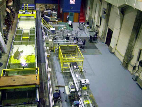
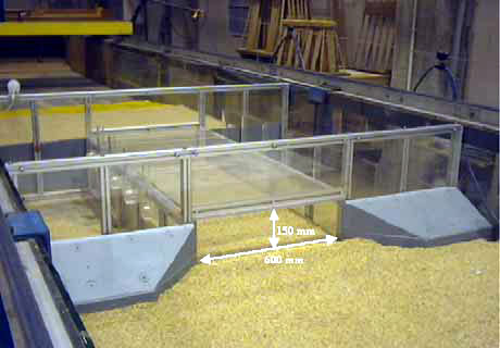
Hydraulic Flume

The experiments were conducted in a 21.34- by 1.83-meter (m) (70- by 6-feet (ft)) rectangular flume with a 2.4- by 1.83-m (8- by 6-ft) recessed section to allow for scour hole formation (figure 1). A 9.14-m (30-ft) approach section from the head box to the test section consisted of a plywood floor constructed 0.1 m (4 inches) above the stainless steel flume bottom. The plywood floor was coated with a layer of epoxy paint and sand to approximate the roughness of the sand bed in the test section. The walls of the flume were made of a smooth glass. The flume was set at a constant slope of 0.04 percent, and the depth of flow was controlled with an adjustable tailgate located at the downstream end of the flume. Flow was supplied by a 0.3-cubic meter per second (m³/s) (10-cubic foot per second (ft³/s)) pumping system. The discharge was measured with an electromagnetic flow meter.

Electromagnetic Velocity Meter Operation

A 13-millimeter (mm) (0.507-inch) spherical electromagnetic velocity sensor (Marsh-McBirney 523) was used to measure equivalent two-directional mean velocities in a plane parallel to the flume bed. A fluctuating magnetic field was produced in the fluid surrounding the spherical sensor that was orthogonal to the plane of four carbon-tipped electrodes. As a conductive fluid passed around the sensor, an electric potential was produced proportional to the product of the fluid velocity component tangent to the surface of the sphere and normal to the magnetic field and the magnetic field strength. The four carbon-tipped electrodes detected the voltage potential created by the flowing water. The voltage potential produced was proportional to the velocity of the fluid flowing in the plane of the electrodes. Two orthogonal velocity components in the plane of the electrodes were measured.

Particle Image Velocimetry

Particle image velocimetry (PIV) was used to verify and modify the prescour velocity field assumptions and equations developed by Chang (i.e., V_R-values as presented in Phase I of the study).(1) These experimental results were then used to derive new regression equations for the maximum depth of scour and for riprap design.

Postprocessing and Data Analysis

Postprocessing and data analysis were performed using the LabVIEW^™ graphical programming technique for building applications such as testing and measurement, data acquisition, instrument control, data logging, measurement analysis, and report generation. LabVIEW programs are called virtual instruments (VIs) because their appearance and operation imitate physical instruments such as oscilloscopes and multimeters. Every VI uses functions that manipulate input from the user interface or other sources and displays that information or moves it to other files or other computers.

MODEL BOTTOMLESS CULVERT SHAPES

Phase I

Three bottomless culvert shapes were constructed and tested:⁽¹⁾ a rectangular model with a width of 0.61 m (2 ft) and a height of 0.46 m (1.5 ft),⁽²⁾ a CON/SPAN^® model with a width of 0.61 m and a height of 0.45 m (1.46 ft), and⁽³⁾ a CONTECH^® model with a width of 0.61 m and a height of 0.42 m (1.36 ft).(1) All three models were evaluated with 45-degree wingwalls and without wingwalls. The models were constructed of Plexiglas^®. Marine plywood was used for the headwalls and wingwalls of the models. The models were mounted in the centerline of the flume. The data derived from testing these culvert shapes were part of the dataset that was used to test the MDSHA (Chang) Method.

Phase II

The laboratory model for this phase consisted of a rectangular bottomless culvert with a width of 0.60 m (2 ft) and a height of 0.15 m (0.49 ft) that was mounted in the centerline of the flume. Figure 2 shows that the culvert and headwall of the model was constructed of Plexiglas or marine plywood, and that the wingwalls were made from marine plywood, Plexiglas, or foam. This model was used to evaluate the outlet scour for a variety of wingwall angles.

Figure 2. Photo. Rectangular culvert.

EXPERIMENTAL PARAMETERS

Approach Flow and Sediment Sizes

Steady flow experiments were conducted for approach flow depths ranging from 0.102 m to 0.325 m (0.33 ft to 1.1 ft) and approach velocities ranging from 0.041 to 0.366 m/s (0.13 to 1.2 ft/s). The discharges to obtain the approach flow conditions varied from approximately 0.024 to 0.14 m³/s (0.9 to 5 ft³/s). The particle size (D₅₀) used during the Phase I scour experiments varied from 1.2 to 3.0 mm (0.047 to 0.117 inches). The particle size for Phase II was 1.2 mm (0.047 inches).

Outlet Scour

Steady flow experiments were conducted for approach flow depths ranging from 0.10 to 0.23 m (0.33 to 0.75 ft) and approach velocities ranging from 0.07 to 0.16 m/s (0.23 to 0.52 ft/s). The discharges to obtain the approach flow conditions varied from approximately 0.026 to 0.080 m³/s (0.9 to 3 ft³/s). The particle size (D₅₀) was set at 2.0 mm (0.078 inches) for the outlet scour experiments. Several scour countermeasure configurations were tested, including varying wingwall angles, the use of pile dissipators, and the MDSHA Standard Plan, which employs wingwalls at the inlet and outlet of the culvert and lines the wingwalls and the inside walls of the culvert with riprap having a particle size (D₅₀) of 25.4 mm (1 inch).

Riprap Experiments

Riprap experiments were conducted for uniform particle sizes of 12 and 16 mm (0.47 and 0.62 inch). The velocity was increased incrementally until discernible areas of particles were dislodged, which was considered to define the failure condition for that particle size. Because of time constraints, riprap experiments (figure 3) were conducted for the rectangular culvert with vertical headwalls only. Vertical headwalls were considered a worst-case condition, and wingwalls should reduce the riprap size determined from these experiments.

Figure 3. Photo. Riprap test for a rectangular culvert.

Cross Vane Analysis

For the analysis of the cross vanes, the flow velocity was set at 0.17 m/s (0.557 ft/s) and the flow depth was set at 0.152 m (0.5 ft). The particle size (D₅₀) was set at either 0.3 mm (0.012 inch) or 25.4 mm (1 inch). The model scale was 1:12.

Test Matrix

The scour, riprap, and cross vane experiments for bottomless culverts are summarized in the test matrix in table 1.

Previous | Contents | Next