U.S. Department of Transportation
Federal Highway Administration
1200 New Jersey Avenue, SE
Washington, DC 20590
202-366-4000
Federal Highway Administration Research and Technology
Coordinating, Developing, and Delivering Highway Transportation Innovations
 |
| This report is an archived publication and may contain dated technical, contact, and link information |
|
Publication Number: FHWA-HRT-05-054
Date: September 2005 |
|||||||||||||||||||||||||||||||||||||||||||||||||||||||||||||||||||||||||||||||||||||||||||||||||||||||||||||||||||||||||||||||||||||||||||||||||||||||||||||||||||||||||||||||||||||||||||||||||||||||||||||||||||||||||||||||||||||||||||||||||||||||||||||||||||||||||||||||||||||||||||||||||||||||||||||||||||||||||||||||||||||||||||||||||||||||||||||||||||||||||||||||||||||||||||||
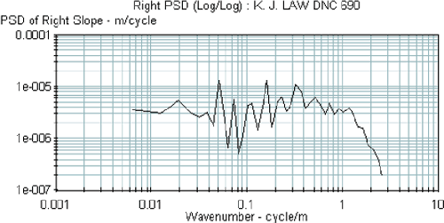
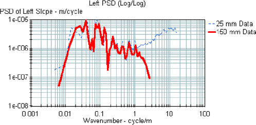
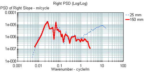
Quantification of Smoothness Index Differences Related To Long-Term Pavement Performance Equipment TypeChapter 5. Data Collection Characteristics and Comparison Of Data Collected By LTPP'S ProfilersCHARACTERISTICS OF DATA COLLECTED BY LTPP'S PROFILERSK.J. Law Engineers DNC 690 ProfilerThe DNC 690 profiler collected profile data at 25.4-mm (1-inch) intervals, and then applied a 304.8-mm (12-inch) moving average onto the data and recorded the data at 152.4-mm (6-inch) intervals. The data collected by this profiler at LTPP sections and the IRI values computed from the profile data are available in the LTPP database. Figure 19 shows a PSD plot of the data collected by this profiler. The PSD plot shows a sharp drop after a wave number of 1 cycle/m (0.3 cycle/ft), which corresponds to a wavelength of 1 m (3 ft). This sharp drop in the PSD plot is an indication that a moving average has been applied to the profile data. The application of the moving average onto the profile data attenuates wavelengths less than 1 m (3 ft). 1 cycle/m = 0.3 cycle/ft Figure 19. PSD plot of data collected by the K.J. Law Engineers DNC 690 profiler. K.J. Law Engineers T-6600 ProfilerThe T-6600 profiler recorded profile data at 25-mm (1-inch) intervals. In the LTPP program, these data are processed using the ProQual software, which applies a 300-mm (11.8-inch) moving average onto the 25-mm (1-inch) interval profile data, and then extracts profile data points at 150-mm intervals. ProQual computes the IRI using these averaged data. The IRI values and the averaged 150-mm (5.9-inch) interval profile data for LTPP sections are available in the LTPP database. Figure 20 shows a PSD plot of the 25-mm (1-inch) data collected by the T-6600 profiler and the PSD plot of the same data after it has been processed using ProQual. Figure 20 shows that there is a significant difference in the profile content between the two profilers for wave numbers greater than 1 cycle/m (0.3 cycle/ft), which corresponds to wavelengths less than 1 m (3 ft). The sharp dropoff seen in the PSD plot for 150-mm (5.9-inch) data for wave numbers greater than 1 cycle/m (0.3 cycle/ft) occurs because the moving average attenuates wavelengths less than 1 m (3 ft) in the profile. 1 cycle/m = 0.3 cycle/ft Figure 20. PSD plot of data collected by the K.J. Law Engineers T-6600 profiler. International Cybernetics Corporation ProfilerThe ICC profilers do not record profile data, but rather record the data collected by the height sensors, accelerometers, and the DMI. These data can be used to generate profiles with a 25-mm (1-inch) sampling interval. In the LTPP program, these 25-mm (1-inch) data are processed using the ProQual software, which uses the same procedure as described for the T-6600 profiler. As in the case of the T-6600 profiler, IRI is computed using the averaged data that are at 150-mm (5.9-inch) intervals. The computed IRI values and the averaged profile data for LTPP sections are available in the LTPP database. Figure 21 shows a PSD plot of the 25-mm (1-inch) data collected by the ICC profiler and the PSD plot of the same data after it had been processed using ProQual. The trend between the 25-mm (1-inch) data and the 150-mm (5.9-inch) data seen in this figure is similar to the trend that was observed for the T-6600 profiler, where the application of the moving average caused profile features that have a wave number greater than 1 cycle/m (0.3 cycle/ft) to become attenuated. COMPARISON OF K.J. LAW ENGINEERS DNC 690 AND T-6600 PROFILERSComparison of Profile DataThe DNC 690 profiler recorded profile data at 152.4-mm (6-inch) intervals, while the T-6600 profiler recorded profile data at 25-mm (1-inch) intervals. The DNC 690 and T-6600 profilers applied a 91-m (300-ft) and 100-m (328-ft) upper-wavelength cutoff filter to the profile data, respectively.
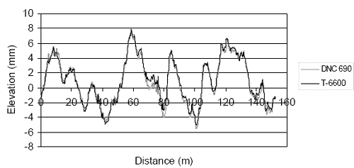
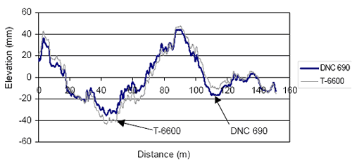
1 cycle/m = 0.3 cycle/ft Figure 21. PSD plot of data collected by the ICC profiler. Figure 22 shows overlaid profile plots of data collected at the same site by the DNC 690 and T-6600 profilers. These data are from the smooth AC section that was used by the North Central region for the 1996 profiler verification test.(24) Figure 23 shows a similar plot at the rough AC section used by the North Central region for the same study.
2.54 mm = 1 inch Figure 22. Data collected by the North Central K.J. Law Engineers DNC 690 and T-6600 profilers at the smooth AC site during the 1996 verification test.
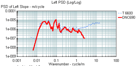
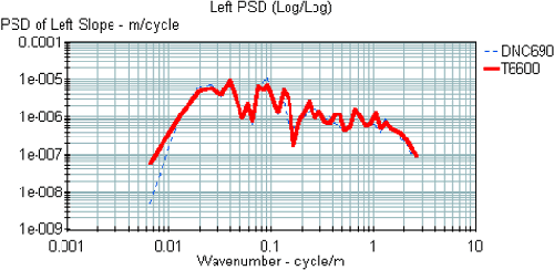
2.54 mm = 1 inch Figure 23. Data collected by the North Central K.J. Law Engineers DNC 690 and T-6600 profilers at the rough AC site during the 1996 verification test. The data collected by the two profilers overlay extremely well at the smooth AC section, while at the rough AC section, the agreement is less when compared to the agreement seen at the smooth AC section. At the rough AC section, although there is a slight shift between the two profiles, an evaluation of the profile data using filtering techniques shows that similar profile features are captured by both profilers. The overall shape of a profile plot primarily depends on the long-wavelength content in the profile. There is a slight difference in the long-wavelength cutoff limit used by the two profilers, which can cause some differences to occur in the profile plots. The long-wavelength content at the rough AC site is higher than that at the smooth AC site and, thus, differences among the profiles are seen more clearly at the rough AC site. These observations, as well as a comparison of other data collected during the 1996 verification test, indicate that the same upper-wavelength cutoff filtering technique appears to have been used with the DNC 690 and T-6600 profilers. Figure 24 shows PSD plots of left-wheelpath data collected by the DNC 690 profiler, which has a sampling interval of 152.4 mm (6 inches), and the T-6600 profiler, which has a sampling interval of 25 mm (1 inch), at the smooth AC site in the North Central region during the 1996 verification test. The PSD plots show good agreement, except for wave numbers greater than 1 cycle/m (0.3 cycle/ft), which corresponds to wavelengths less than 1 m (3 ft). In this waveband range, the profile content in the DNC 690 profiler is attenuated when compared to the T-6600 profiler. This attenuation is caused by the moving average filter that is applied to the DNC 690 profiler data before saving the data. Figure 25 shows the PSD plot of the two data sets whose PSD plots are shown in figure 24, except that the data shown for the T-6600 profiler are the data that were obtained after the 25-mm (1-inch) data were processed using ProQual. The application of the 300-mm (11.8-inch) moving average onto the 25-mm (1-inch) T-6600 profiler data attenuates wavelengths less than 1 m (3 ft), which corresponds to wave numbers greater than 1 cycle/m (0.3 cycle/ft). The two PSD plots shown in figure 25 indicate good agreement. A review of similar plots for other data collected during the 1996 verification test showed similar trends. These results confirm that the DNC 690 profiler applied a 304.8-mm (12-inch) moving average onto the data before saving the data. Since the PSD plots for the two profilers agree well through a range of 0.025 to 1 cycle/m (0.008 to 0.3 cycle/ft), which corresponds to wavelengths between 1 and 40 m (3 and 130 ft), the IRI values of the two profilers are expected to agree closely.
1 cycle/m = 0.3 cycle/ft Figure 24. PSD plot of data collected by the K.J. Law Engineers DNC 690 and T-6600 profilers.
1 cycle/m = 0.3 cycle/ft Figure 25. PSD plots of K.J. Law Engineers DNC 690 profiler data and ProQual-processed T-6600 profiler data. The PSD plots also indicate that the spectral content of the data collected at the same site by the two profilers was similar. This indicates that the profile features that are recorded by the two profilers are similar. (Note: These observations are only valid when the DNC 690 profiler data are compared to ProQual-processed T-6600 profiler data. If 25-mm (1-inch) T-6600 profiler data are compared to DNC 690 profiler data, differences among the profile data will be seen for wave numbers greater than 1 cycle/m (0.3 cycle/ft).) The PSD plots also indicated good agreement between the two profilers for low wave numbers (long wavelengths), which is an indication that the filtering technique used by the two profilers for the upper-wavelength cutoff is similar. The slight differences seen in the PSD plots for the low wave numbers (long wavelengths) are probably related to the different upper-wavelength cutoff values that were used in the two profilers, which are 91 m (300 ft) for the DNC 690 profiler and 100 m (328 ft) for the T-6600 profiler. Comparison of IRI ValuesWhen comparison testing between the two profilers is performed, the profiler driver should do the following two tasks accurately:
If the profiler driver does not correctly align the profiler along the wheelpaths, the longitudinal path followed by the sensors of the different profilers will be different. This can cause IRI obtained from the different profilers to vary. After aligning the profiler along the wheelpaths, the driver should also follow a consistent path within the test section without lateral wander. If the is variability in the path that is followed within the section, it can result in differences in IRI when the two profilers are being compared. The ability of a driver to correctly align the profiler along the wheelpaths and to follow a consistent path within the section can vary among drivers. Drivers who are more experienced in profiling can probably do these two tasks much better than a driver who is inexperienced in profiling. A driver who is experienced in profiling probably will also be able to follow a more consistent path when obtaining repeat measurements at a site than a person who does not have much experience in operating the profiler. The ability of a driver to correctly align the profiler along the wheelpaths and to follow a consistent path within the section can vary among drivers. Drivers who are more experienced in profiling can probably do these two tasks much better than a driver who is inexperienced in profiling. A driver who is experienced in profiling probably will also be able to follow a more consistent path when obtaining repeat measurements at a site than a person who does not have much experience in operating the profiler. Not following the correct wheelpath, or variability within the section during profiling, will usually have a greater impact on the IRI for sections that have distresses. This is because, in such sections, lateral variations can cause certain pavement features either to be included or missed in the profile, thus affecting the IRI. The effect of lateral wander is an issue that can sometimes complicate the analysis when the IRI from different profilers are compared. A study performed for an NCHRP project found that variations in the longitudinal path that is followed during profiling could have a significant effect on IRI.(1) In this study, the effect of lateral variations in profiling was studied at seven test sections. The percent change in IRI that was obtained for each wheelpath at the test sections for a 0.3-m (1-ft) lateral shift in the longitudinal path to the left and to the right is shown in table 3. As shown in this table, the percent change in IRI will vary for different pavements. Some pavements showed extremely large variations in IRI for a 0.3-m (1-ft) shift from the wheelpath. Generally, the percent change in IRI that was observed along the left wheelpath was less than that obtained for the right wheelpath.
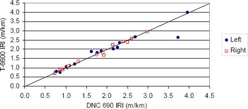
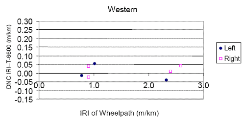
1 m = 3.28 ft After each regional contractor accepted delivery of the T-6600 profiler in 1996, they performed a comparison of this profiler and the DNC 690 profiler. Four test sections were used in each region to perform this comparison. (See references 24, 25, 26, and 27.) The results obtained from this test are described in appendix B. In the reports prepared by the regional contractors, the average IRI value for a wheelpath from the multiple runs that were performed at a site was computed using different procedures. In this research project, a consistent method was used on data obtained from all four regions to compare the IRI values between the DNC 690 and T-6600 profilers. The IRI values obtained for sequence 2 testing were used in this analysis (except at site 1 in the Western region for the DNC 690 profiler, where sequence 1 values were used because sequence 2 data had saturation spikes). The average IRI for each wheelpath at each test section was computed using the IRI for the five runs that had the least standard deviations in IRI for the mean IRI (i.e., the average IRI for the left and right wheelpaths). The computed average IRI values for both profilers for all regions are shown in table 4. When all 4 regions were considered, there were a total of 16 test sites (32 wheelpaths) where IRI comparisons between the 2 profilers could be made. Figure 26 shows the IRI relationship between the two profilers, where data obtained for 32 wheelpaths are shown. There is very good agreement in the IRI values obtained by the two profilers, except for one case along the left wheelpath. This data point corresponds to the left wheelpath of site 2 in the Western region. An evaluation of the data indicated that the data collected by the DNC 690 profiler had a significant number of spikes that were caused by sunlight being picked up by the sensor, which resulted in a high IRI value. The correlation coefficient for the data shown in figure 26 is 0.98.
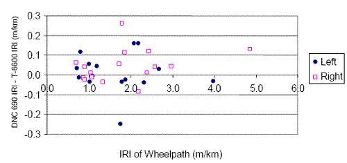
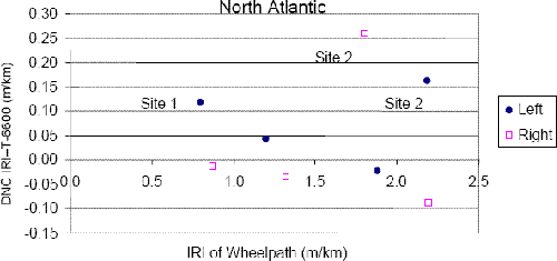
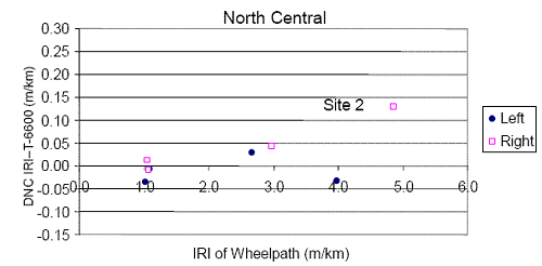
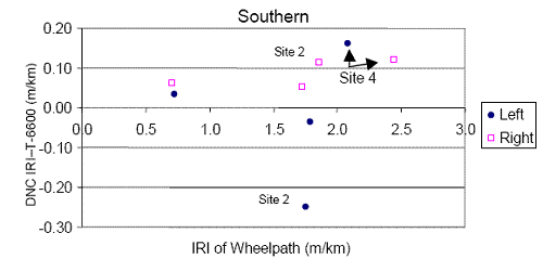
1 m/km = 5.28 ft/mi 1 m/km = 5.28 ft/mi Figure 26. Relationship between IRI from the K.J. Law Engineers DNC 690 and T-6600 profilers. The difference in IRI between the DNC 690 and T-6600 profilers (DNC 690 IRI — T-6600 IRI) was computed along each wheelpath for all of the test sections. These data are shown in figure 27 as a function of the IRI for the wheelpath, where the IRI for the wheelpath was computed by averaging the IRI obtained for that wheelpath by the DNC 690 and T-6600 profilers. Of the 32 available cases, the difference in IRI was within ±0.10 m/km (±6 inches/mi) for 23 cases. For six cases, the difference was between 0.10 and 0.20 m/km (6 and 13 inches/mi). There was one case where the difference was between -0.20 and -0.30 m/km (-13 and -19 inches/mi), one case where the difference was between 0.20 and 0.30 m/km (13 and 19 inches/mi), and one case where the difference was greater than 1.1 m/km (70 inches/mi) (this data point is not shown in figure 27). 1 m/km = 5.28 ft/mi Figure 27. Differences in IRI between the K.J. Law Engineers DNC 690 and T-6600 profilers: All regions. An investigation was performed separately for each region to identify the cause of the difference in IRI between the two profilers for cases where the difference in IRI was outside ±0.10 m/km (±6 inches/mi). In each region, the difference in IRI between the DNC 690 and T-6600 profilers (DNC 690 IRI — T-6600 IRI) for each wheelpath was plotted as a function of the IRI for the wheelpath, with the IRI for the wheelpath computed by averaging IRI obtained by the two profilers for that wheelpath. North Atlantic RegionFigure 28 shows the difference in IRI from the DNC 690 and T-6600 profilers at the test sections tested by the North Atlantic profilers as a function of the IRI for the wheelpath. A difference in IRI between the DNC 690 and T-6600 profilers (DNC 690 — IRI — T-6600 IRI) that was outside ±0.10 m/km (±6 inches/mi) was observed for the following three cases: (1) left wheelpath of site 1 (a difference of 0.12 m/km (8 inches/mi)), (2) left wheelpath of site 2 (a difference of 0.16 m/km (10 inches/mi)), and (3) right wheelpath of site 2 (a difference of 0.26 m/km (16 inches/mi)). Site 1: The left-wheelpath IRI from the DNC 690 profiler was 0.12 m/km (8 inches/mi) higher than IRI obtained by the T-6600 profiler. The DNC 690 profiler conducted six runs on this section. IRI along the left wheelpath for these six runs ranged from 0.83 to 0.87 m/km (53 to 55 inches/mi). The T-6600 profiler conducted nine runs at this site, and the left-wheelpath IRI for eight runs ranged from 0.72 to 0.77 m/km (46 to 49 inches/mi); however, there was one run that had an IRI of 0.85 m/km (54 inches/mi). The roughness profile of this run overlaid extremely well with the roughness profiles obtained by the DNC 690 profiler. This indicates that the probable cause of the difference in IRI between the two profilers was a difference in the paths that were followed during profiling. 1 m/km = 5.28 ft/mi Figure 28. Differences in IRI between the K.J. Law Engineers DNC 690 and T-6600 profilers: North Atlantic region. Site 2: IRI from the DNC 690 profiler was higher than IRI from the T-6600 profiler by 0.16 m/km (10 inches/mi) and 0.26 m/km (16 inches/mi) for the left and right wheelpaths, respectively. This analysis used IRI values obtained during sequence 2 testing. The average IRI from the T-6600 profiler from sequence 1 testing at this site, along the left and right wheelpaths, were 2.21 m/km (140 inches/mi) and 1.89 m/km (120 inches/mi), respectively. These values compare extremely well with the IRI values obtained for the left and right wheelpaths by the DNC 690 profiler (2.27 m/km (144 inches/mi) and 1.93 m/km (122 inches/mi), respectively). This section had significant transverse and longitudinal cracking along both wheelpaths throughout the test section. Thus, the differences in IRI that were observed between the two profilers for sequence 2 testing are attributed to variations in the wheelpaths followed by the two profilers. North Central RegionFigure 29 shows the differences in IRI from the DNC 690 and T-6600 profilers at the test sections in the North Central region as a function of the IRI for the wheelpath. A difference in IRI between the DNC 690 and T-6600 profilers that was outside ±0.10 m/km (±6 inches/mi) was observed only along the right wheelpath at site 2, where the IRI from the DNC 690 profiler was higher than that from the T-6000 profiler by 0.13 m/km (8 inches/mi). The right wheelpath at this site is extremely rough. The right-wheelpath IRI for the five selected runs from the DNC 690 profiler ranged from 4.77 to 4.96 m/km (302 to 314 inches/mi), while the IRI for the five selected runs from the T-6600 profiler ranged from 4.74 to 4.81 m/km (301 to 305 inches/mi). These ranges for the two profilers have some overlap. The difference in IRI between the two profilers at this site is attributed to variations in the wheelpaths. 1 m/km = 5.28 ft/mi Figure 29. Differences in IRI between the K.J. Law Engineers DNC 690 and T-6600 profilers: North Central region. Southern RegionFigure 30 shows the difference in IRI from the DNC 690 and T-6600 profilers at the test sections tested by the Southern profilers as a function of the IRI for the wheelpath. Differences in IRI between the DNC 690 and T-6600 profilers (DNC 690 — IRI — T-6600 IRI) that were outside ±0.10 m/km (±6 inches/mi) were observed for the following four cases: (1) left wheelpath of site 2 (a difference of -0.25 m/km (-16 inches/mi)), (2) right wheelpath of site 2 (a difference of 0.11 m/km (10 inches/mi)), (3) left wheelpath of site 4 (a difference of 0.16 m/km (10 inches/mi)), and (4) right wheelpath of site 4 (a difference of 0.12 m/km (7 inches/mi)). Site 2: At this site, IRI from the DNC 690 profiler was lower than that from the T-6600 profiler along the left wheelpath by 0.25 m/km (16 inches/mi), but higher than that obtained by the T-6600 profiler by 0.11 m/km (7 inches/mi) along the right wheelpath. The T-6600 profiler conducted nine runs at this site. Along the left wheelpath, the IRI for the nine runs ranged from 1.80 to 2.00 m/km (114 to 127 inches/mi), while along the right wheelpath, the IRI ranged from 1.70 to 1.86 m/km (108 to 118 inches/mi). This indicates there is some transverse variability at this site. A comparison of the profile data from the T-6000 and DNC 690 profilers indicated that there were localized differences between the profile data and that these caused the difference in the IRI from the profilers. The difference in IRI between the two profilers has opposite signs for the two wheelpaths. This is usually an indication that the difference in IRI between the two profilers is probably related to variations in the profiled paths. No explanation other than variability between the profiled paths can be offered to explain the difference in IRI between the two profilers at this site. 1 m/km = 5.28 ft/mi Figure 30. Differences in IRI between the K.J. Law Engineers DNC 690 and T-6600 profilers: Southern region. Site 4: IRI from the DNC 690 profiler at this site was higher than that obtained by the T-6600 profiler by 0.16 m/km (10 inches/mi) and 0.12 m/km (8 inches/mi) along the left and right wheelpaths, respectively. An evaluation of the roughness profile for the left wheelpath indicated that most of the difference in roughness between the two profilers was occurring between 140 m (459 ft) and the end of the section. This was caused by differences in the way a feature, which was located at approximately 145 m (476 ft), was being measured by the two profilers. An evaluation of the roughness profiles for the right wheelpath also showed some localized variations in roughness that occurred because of differences in the way features were measured by the two profilers. Because this site is fairly rough, with left- and right-wheelpath IRI values of approximately 2.10 and 2.14 m/km (133 and 152 inches/mi), respectively, variations in the profiled paths are probably the cause of the difference in IRI between the two profilers. Western RegionFigure 31 shows the difference in IRI from the DNC 690 and T-6600 profilers at the sections tested by the two Western profilers as a function of the IRI for the wheelpath. The difference in IRI between the two profilers was within ±0.10 m/km (±6 inches/mi) for all of the cases except one. This case was along the left wheelpath at section 2, where the difference in IRI was 1.1 m/km (70 inches/mi). This occurred because data collected by the DNC 690 profiler was contaminated by saturation spikes. This data point is not shown in figure 31. Cross Correlation of IRIThe cross-correlation technique provides a method to compare the magnitude and the spatial distribution of IRI between two devices. This technique was used to compare IRI obtained by the DNC 690 and T-6600 profilers using data obtained during the 1996 verification testing in the North Central and Western regions. When using the cross-correlation technique, the DNC 690 profiler was considered to be the "correct" device and, thus, the analysis will indicate how well the T-6600 profiler reproduced the results from the DNC 690 profiler. 1 m/km = 5.28 ft/mi Figure 31. Differences in IRI between the K.J. Law Engineers DNC 690 and T-6600 profilers: Western region. One representative run was selected for each profiler at each site to perform this analysis. In this analysis, for the T-6600 profiler, the ProQual-processed averaged data that are at 150-mm (5.9-inch) intervals was used, while for the DNC 690 profiler, the 152.4-mm (6-inch) data obtained by the profiler was used. Because the data collected by the DNC 690 profiler is considered to be the correct data, any deviations in the path followed by the T-6600 profiler from the path followed by the DNC 690 profiler will affect the results. The results of the crosscorrelation analysis are presented in table 5.
1 m/km = 5.28 ft/mi The sensor spacing for the two North Central profilers was different. During testing, the two profilers aligned the right sensor along a similar path using a camera system. The two North Central profilers had very high cross-correlation values along the right wheelpath where the camera system was used to judge the wheelpath. This indicates excellent agreement in both the IRI magnitude and IRI distribution along that path for the two profilers. The two North Central profilers also showed good cross-correlation values along the left wheelpath, too, although the values were slightly less than those obtained for the right wheelpath. The two profilers in the Western region also had high cross-correlation values at the majority of the sections. The data collected along the left wheelpath at site 2 by the DNC 690 profiler were contaminated with saturation spikes, thus, a low cross-correlation value was obtained for this case. The cross-correlation values at site 3 were somewhat lower than the values obtained for the other sites. Site 3 is a concrete site, and evaluation of the profile data indicated that the amount of slab curling that was present when the two profilers measured the site was different, and this was the cause of the low cross correlation at this site. Analysis of Variance and Regression Analysis of IRIAn analysis of variance (ANOVA) was performed using the IRI values obtained from the 1996 regional testing to determine whether IRI values obtained by the DNC 690 and T-6600 profilers were similar. A two-factor ANOVA was performed using the IRI values obtained for the five runs that were selected for computing the average IRI values shown in table 4. During the 1996 verification test, testing was performed at 16 sections (4 sections per region), and this provided 32 cases (32 wheelpaths) that could be used in the analysis. Because the data for the left wheelpath at site 2 in the Western region for the DNC 690 profiler were erroneous, these data were omitted from the analysis. The ANOVA indicated that the profilers were significant at a significance level of 0.05. Another ANOVA was performed by omitting the data for the left wheelpath in the North Central region. This was done because the two profilers in the North Central region have different sensor spacing, and they were aligned along the right wheelpath during testing. This analysis also found that the profilers were significant at a significance level of 0.05. Thereafter, separate ANOVAs were performed for each region. The only case where the profilers were not significant was in the Western region. Thereafter, for each region, separate ANOVAs were performed for each wheelpath. The only cases where the profilers were not significant at a significance level of 0.05 were for the left and right wheelpaths in the Western region, and for the left wheelpath in the North Central region. A regression analysis was performed for the IRI from the DNC 690 and T-6600 profilers. The IRI for the five runs that were selected at each section to compute the average IRI value in the previous analysis were used in the regression. This provided 155 pairs of data for the regression (i.e., four regions x four sections per region x two wheelpaths per section x five runs per section, less the erroneous left-wheelpath runs at section 2 in the Western region). The following relationship was obtained from the regression: IRI (T-6600) = 0.982 IRI (DNC 690) + 0.004 (1) where:
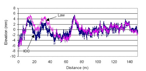
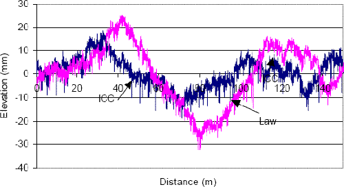
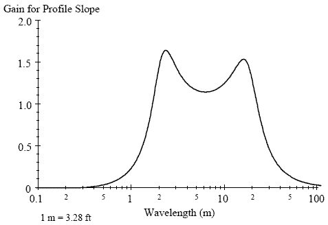
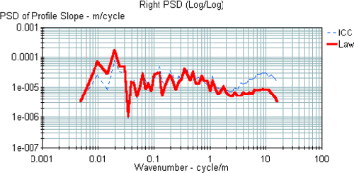
The regression analysis indicated that IRI from the two profilers were extremely similar; however, IRI obtained from the DNC 690 profiler was predicted to be slightly higher than that obtained from the T-6600 profiler. COMPARISON OF K.J. LAW ENGINEERS T-6600 AND ICC PROFILERSComparison of Profile DataThe data obtained from the 2002 verification test were used for this analysis. Both profilers applied a 100-m (328-ft) upper-wavelength cutoff filter onto the data. The data collected by both profilers along each wheelpath at each site were overlaid to evaluate differences in the data. At some sites, the profiles overlaid extremely well; however, at many sites, there were significant differences among the profiles. Figure 32 shows an example of a case where close agreement was obtained between the profile data from the two profilers. Figure 33 shows an example of a case where there were significant differences between the profile plots. The data shown in figures 32 and 33 are the 25-mm (1-inch) left-wheelpath data collected by the two Western profilers during the 2002 verification test at LTPP sites 320209 and 069107, respectively. 25.4 mm = 1 inch Figure 32. Comparison of ICC and K.J. Law Engineers profiles: Western site 320209. An evaluation of all data collected for the 2002 verification test indicated that the profile plots from the two profilers usually overlaid well at sites that did not have much long-wavelength content. However, differences between the profile plots were noticeable at sites that had more long-wavelength content. An evaluation of the profile data using filtering techniques indicated that profile features that were present on the pavement were being measured similarly by both profilers. These observations indicate that there are differences in the long-wavelength data collected by the two profilers. The differences in the long wavelengths appear to be occurring for wavelengths greater than approximately 40 m (131 ft). 25.4 mm = 1 inch Figure 33. Comparison of ICC and K.J. Law Engineers profiles: Western site 069107. The response of the quarter car filter that is used in the IRI computation procedure to different wavelengths is shown in figure 34.(2) The amplitude of the output sinusoid is the amplitude of the input multiplied by the gain shown in the figure, which is dimensionless. IRI is primarily influenced by wavelengths ranging from 1.2 to 30.5 m (4 to 100 ft).(2) However, there is still some response to wavelengths outside this range. The IRI filter has a maximum sensitivity to sinusoids with wavelengths of 2.4 and 15.4 m (7.9 and 50.5 ft). The response is down to 0.5 for wavelengths of 1.2 and 30.5 m (4 and 100 ft).(2) 1 m = 3.28 ft Figure 34. Response of the IRI filter.(2) IRI obtained by the T-6600 and ICC profilers during the 2002 verification test showed good agreement.(28) Although there are differences in the long wavelengths between the two profilers, good agreement in IRI between the two profilers indicates that the profilers are collecting similar data within the wavelength range that is influencing the IRI that was described previously. The K.J. Law Engineers profiler uses a Butterworth filter for long-wavelength cutoff, while the ICC profiler uses a cotangent filter. Although both profilers are using an upper-wavelength cutoff filter of 100 m (328 ft), differences in the filtering techniques used by the two profilers are causing some differences in the long-wavelength data between the two profilers. An evaluation of the filtering techniques indicated that the Butterworth filter makes a much sharper transition from wavelengths that are unmodified to wavelengths that are eliminated than the cotangent filter, and this causes differences in the long wavelengths to occur between the two profilers. Figure 35 shows a typical PSD plot that was obtained when the 25-mm (1-inch) data from the ICC and K.J. Law Engineers profilers were compared. The data shown in figure 35 are those obtained by the two North Central profilers at site 5 (which has a chip seal) during the 2002 verification test. The two PSD plots show good agreement between wave numbers of 0.025 and 1 cycle/m (0.008 and 0.305 cycle/ft), which correspond to wavelengths between 40 and 1 m (131 and 3 ft). However, there are differences between the profilers for wave numbers less than 0.025 cycle/m (0.008 cycle/ft), which corresponds to wavelengths greater than 40 m (131 ft), and wave numbers greater than 1 cycle/m (0.3 cycle/ft), which corresponds to (wavelengths less than 1 m (3 ft).
1 cycle/m = 0.3 cycle/ft Figure 35. PSD plot of 25-mm (1-inch) data collected by the North Central ICC and K.J. Law Engineers profilers at the chip-seal section during the 2002 verification test. An examination of PSD plots of data collected by the ICC and K.J. Law Engineers profilers during the 2002 regional comparison indicated the following:
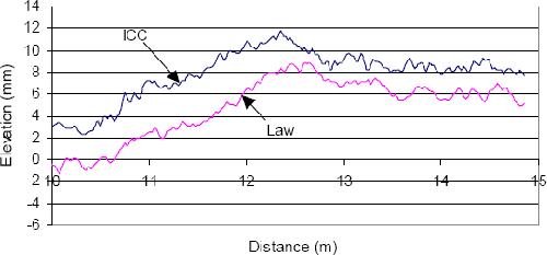
A closeup view of the 25-mm (1-inch) profile data collected by the two profilers at the site (whose PSD plot is shown figure 35) is shown in figure 36. Figure 36 indicates that the profile recorded by the ICC profiler shows more profile details compared to those recorded by the K.J. Law Engineers profiler. This is why the PSD plots shown in figure 35 indicate a difference between the two profilers for wave numbers greater than 1 cycle/m (0.3 cycle/ft). 1 inch = 25.4 mm Figure 36. Closeup view of 25-mm (1-inch) profile data collected by North Central ICC and K.J. Law Engineers profilers on a chip-seal pavement. When ProQual processes the 25-mm (1-inch) data by applying a 300-mm (11.8-inch) moving average, the short-wavelength features that have wavelengths less than 1 m (3 ft) will become attenuated and the PSD plots for the two profilers will show better agreement for wave numbers greater than 1 cycle/m (0.3 cycle/ft). An analysis was performed to investigate the differences between the two profilers in measuring short wavelengths. The data collected by the North Central profilers during the 2002 regional verification test were used for this analysis. At each site, one run from each profiler was selected, and the analysis was performed on the left-wheelpath data. The analysis was performed on the first 76 m (249 ft) of the data from the site. The profile data were filtered to get rid of the long wavelengths, so that only the short wavelengths would be present in the profile. Thereafter, the standard deviations of the filtered elevation values were computed. The results from this analysis are presented in table 6.
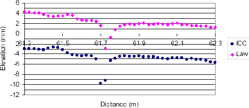
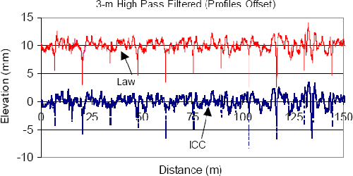
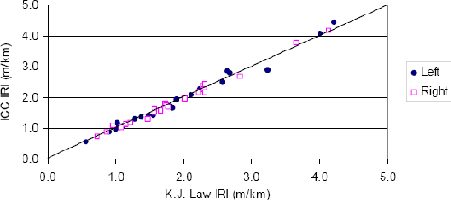
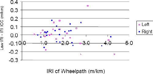
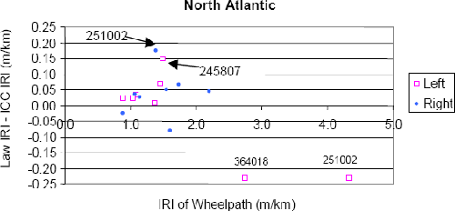
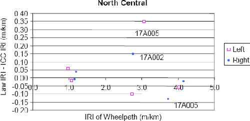
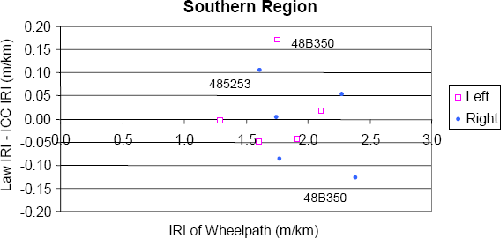
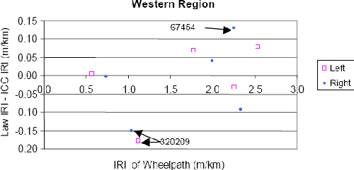
1 inch = 25.4 mm The ICC profiler had higher standard deviations for all of the cases. The data shown in table 6 suggests that the small footprint size of the ICC profiler is measuring more texture-related effects and possibly higher depth at narrow downward features, such as cracks, than that measured by the T-6600 profiler. Comparison of 25-mm (1-inch) data collected by the K.J. Law Engineers and ICC profilers indicated that there were differences in the depth of downward features, such as cracks, that were measured by the profilers at some sites. However, it is unclear if this difference was caused by variations in the paths profiled by the two profilers, or if it was related to differences in the footprint sizes of the two height sensors, or differences in the filtering techniques used by the two profilers. Figure 37 shows a closeup view of the profile data recorded by the two profilers over a joint in a concrete pavement. The data shown in this figure were collected by the two North Central profilers at the rough PCC section during the 2002 verification test. On this pavement, minor variations in the profiled path are not likely to result in a difference in the magnitude of the downward feature measured by the profilers when readings are taken on top of the sealant at a joint. This is because the joint sealant is expected to be at a constant depth from the slab surface over a short lateral distance. However, in cases where there are transverse cracks in the pavement, minor variations in the wheelpaths can result in the crack depth being different. Thus, comparing the magnitude of the downward feature recorded by the two profilers at a joint provides a better choice for comparing the two profilers. The two plots in figure 37 show that the depths of the joint as recorded by the two profilers are very similar; however, the depth recorded by the ICC profiler is slightly higher. 25.4 mm = 1 inch Figure 37. Readings taken over a joint by the two profilers. Figure 38 shows the 25-mm (1-inch) profile data collected by the two profilers at this site after the data have been subjected to a 3-m (10-ft) high-pass filter. The slab length in this concrete pavement is 13 m (43 ft). Figure 38 shows that both profile plots are showing all joint locations, and the depths recorded over the joints by the two profilers are very similar. 25.4 mm = 1 inch Figure 38. Profile data obtained by the ICC and K.J. Law Engineers profilers at a concrete site. Although the profilers output data at 25-mm (1-inch) intervals, the height sensors in the profilers are obtaining data at much closer intervals, and are then averaging the data and using the averaged height-sensor value for computing the profile data at 25-mm (1-inch) intervals. If the profilers were just getting height-sensor data at 25-mm (1-inch) intervals, there is always the possibility that a reading may not be obtained on top of a joint. However, because the height sensors are obtaining readings at much closer intervals than 25 mm (1 inch), a reading is always obtained on top of the joint sealant. When the height-sensor data are averaged to obtain a reading every 25 mm (1 inch), the reading obtained over the joint was of sufficient magnitude for the joint to be clearly seen in the filtered profile. Another interesting observation seen in figure 37 is that the profile data show the joint to be a feature that is spread over a distance of 75 mm (3 inches), when the actual width of the joint is on the order of 10 mm (0.4 inches). The joint appears like this in the profile data because of the averaging procedure that is used on the height-sensor data and possibly because of the application of an anti-aliasing filter onto the profile data. The averaging procedure and the antialiasing filter will also cause some attenuation in the magnitude of the depth of narrow downward features such as joints and cracks. Comparison of IRI ValuesAn analysis of the IRI values obtained from the 2002 verification test was performed to compare IRI values obtained by the two profilers.(28) In the North Central region, testing by both profilers was performed on the same day. In the North Atlantic region, testing at six of the eight sites was performed on the same day by the two profilers, while in the Western region, a similar procedure was followed for three of the five sites. In the Southern region, testing at the sites by the ICC profiler was performed approximately 1.5 months after testing by the K.J. Law Engineers profiler. The IRI values obtained from the testing (average IRI from five runs) and the test dates are presented in appendix B. There were 23 test sites (46 wheelpaths) where IRI comparisons of the two profilers could be made. Figure 39 shows the IRI relationship between the two profilers, where data for 46 wheelpaths are shown. There is very good agreement in IRI between the two profilers, with the correlation coefficient for the two sets of IRI values being 0.99. 1 m/km = 5.28 ft/mi Figure 39. Relationship between IRI from the K.J. Law Engineers and ICC profilers. The difference in IRI between the K.J. Law Engineers and ICC profilers (K.J. Law IRI – ICC IRI) was computed along each wheelpath for all test sections. The differences in IRI are shown in figure 40 as a function of the IRI for the wheelpath, where the IRI for the wheelpath was computed by averaging IRI obtained for that wheelpath by the ICC and K.J. Law Engineers profilers. 1 m/km = 5.28 ft/mi Figure 40. Differences in IRI between the K.J. Law Engineers and ICC profilers. For the 46 cases, the difference in IRI was within ±0.10 m/km (±6 inches/mi) for 33 cases, between 0.10 and 0.20 m/km (6 and 13 inches/mi) for 6 cases, between -0.10 and -0.20 m/km (-6 and -13 inches/mi) for 4 cases, between -0.20 and -0.30 m/km (-13 and -19 inches/mi) for 2 cases, and between 0.30 and 0.40 m/km (19 and 25 inches/mi) for 1 case. An investigation was performed separately for each region to identify the cause of the difference in IRI between the two profilers for cases where the difference in IRI was outside ±0.10 m/km (±6 inches/mi). North Atlantic RegionFigure 41 shows the difference in IRI between the K.J. Law Engineers and ICC profilers at the sections tested by the North Atlantic profilers as a function of the IRI for the wheelpath. 1 m/km = 5.28 ft/mi Figure 41. Differences in IRI between the K.J. Law Engineers and ICC profilers: North Atlantic region. Differences in IRI between the K.J. Law Engineers and ICC profilers (K.J. Law IRI — ICC IRI) that were outside ±0.10 m/km (±6 inches/mi) were observed for the following four cases: (1) left wheelpath of site 251002 (a difference of -0.23 m/km (-15 inches/mi)), (2) right wheelpath of site 251002 (a difference of 0.17 m/km (11 inches/mi)), (3) left wheelpath of site 364018 (a difference of -0.23 m/km (-15 inches/mi)), and (4) left wheelpath of site 245807 (a difference of 0.15 m/km (10 inches/mi)). Site 251002: At this site, the K.J. Law Engineers profiler obtained an IRI that was 0.23 m/km (15 inches/mi) lower than the IRI from the ICC profiler for the left wheelpath, and an IRI that was 0.17 m/km (11 inches/mi) higher than the IRI from the ICC profiler for the right wheelpath. Each profiler conducted nine runs on this section. The IRI for the nine runs from the ICC profiler ranged from 2.58 to 5.03 m/km (164 to 319 inches/mi) for the left wheelpath, and from 1.24 to 1.57 m/km (79 to 100 inches/mi) for the right wheelpath. For the K.J. Law Engineers profiler, the IRI for the nine runs ranged from 2.56 to 4.81 m/km (162 to 305 inches/mi) for the left wheelpath, and from 1.50 to 1.67 m/km (95 to 106 inches/mi) for the right wheelpath. The left wheelpath of this section had significant distress. As indicated from the IRI range that was obtained for the repeat runs, significant variability in IRI can occur at this site because of variability in the profiled path. Investigation of the profile data indicated that the difference in IRI between the two profilers at this site was probably caused by differences in the profiled paths. Site 364018: The K.J. Law Engineers profiler obtained an IRI that was 0.23 m/km (15 inches/mi) less than that obtained by the ICC profiler along the left wheelpath at this section. Each profiler conducted nine runs on this test section. The IRI for the runs for the ICC profiler ranged from 2.64 to 3.18 m/km (167 to 202 inches/mi) for the left wheelpath, and from 2.20 to 2.39 m/km (139 to 151 inches/mi) for the right wheelpath. For the K.J. Law Engineers profiler, IRI ranged from 2.59 to 2.92 m/km (164 to 185 inches/mi) for the left wheelpath, and from 2.23 to 2.36 m/km (141 to 149 inches/mi) for the right wheelpath. There was a major downward feature at a distance of 50 m (164 ft) along the left wheelpath that made a significant contribution to the roughness at this site. Variability in the profiled path that caused this feature to be measured differently had a significant effect on IRI. Investigation of the profile data and roughness profiles at this section indicated that the difference in IRI between the two profilers was caused by variability in the paths followed by the two profilers. Site 245807: Along the left wheelpath at this site, the IRI from the K.J. Law Engineers profiler was 0.15 m/km (10 inches/mi) lower than that obtained by the ICC profiler. An investigation of the profile data did not indicate a clear reason for the cause of this difference. North Central RegionFigure 42 shows the difference in IRI between the K.J. Law Engineers and ICC profilers at the test sections tested by the North Central profilers as a function of the IRI for the wheelpath. Differences in the IRI between the K.J. Law Engineers and ICC profilers (K.J. Law IRI – ICC IRI) that were outside ±0.10 m/km (±6 inches/mi) were observed for the following three cases: (1) right wheelpath of site 17A002 (a difference of 0.15 m/km (10 inches/mi)), (2) left wheelpath of site 17A005 (a difference of 0.35 m/km (22 inches/mi)), and (3) right wheelpath of site 17A005 (a difference of -0.13 m/km (-8 inches/mi)). 1 m/km = 5.28 ft/mi Figure 42. Differences in IRI between the K.J. Law Engineers and ICC profilers: North Central region. Site 17A002: The IRI from the K.J. Law Engineers profiler was higher than that of the ICC profiler by 0.15 m/km (10 inches/mi) along the right wheelpath at this site. However, along the left wheelpath, the IRI from the K.J. Law Engineers profiler was 0.10 m/km (6 inches/mi) lower than that obtained by the ICC profiler. An investigation of the profile data did not indicate a definitive cause for the difference in IRI between the profilers. However, variability in the wheelpath is a likely cause for the difference in IRI. In this case, the difference in IRI between the K.J. Law Engineers and ICC profilers had opposite signs for the wheelpaths (negative for the left wheelpath and positive for the right wheelpath). This is an indication that the two profilers followed different wheelpaths. Site 17A005: The IRI from the K.J. Law Engineers profiler was higher than that obtained by the ICC profiler by 0.35 m/km (22 inches/mi) along the left wheelpath; along the right wheelpath, the IRI from the K.J. Law Engineers profiler was lower than that obtained by the ICC profiler by 0.13 m/km (8 inches/mi). An investigation of the profile data did not indicate a definitive cause for the difference in IRI between the profilers. Since there was a reversal in signs for the difference in IRI for the two wheelpaths as in the previous case, the differences in IRI between the two profilers at this site were probably cased by variability in the paths followed by the two profilers. Southern RegionFigure 43 shows the difference in IRI between the K.J. Law Engineers and ICC profilers at the sections tested by the Southern profilers as a function of the IRI for the wheelpath. Differences in the IRI between the K.J. Law Engineers and ICC profilers (K.J. Law IRI — ICC IRI) that were outside ±0.10 m/km (±6 inches/mi) were observed for the following three cases: (1) left wheelpath of site 48B350 (a difference of 0.17 m/km (11 inches/mi)), (2) right wheelpath of site 48B350 (a difference of -0.13 m/km (-8 inches/mi)), and (3) right wheelpath of site 485253 (a difference of 0.11 m/km (7 inches/mi)). The data recorded by the ICC profiler could not be converted to obtain the 25-mm (1-inch) data, thus, a comparison of the profiles between the ICC and K.J. Law Engineers profilers could not be performed. 1 m/km = 5.28 ft/mi Figure 43. Differences in IRI between the K.J. Law Engineers and ICC profilers: Southern region. At site 48B350, the IRI from the K.J. Law Engineers profiler was higher than that obtained by the ICC profiler by 0.17 m/km (11 inches/mi) along the left wheelpath; however, along the right wheelpath, the IRI from the K.J. Law Engineers profiler was lower than that obtained by the ICC profiler by 0.13 m/km (8 inches/mi). Since the difference in the IRI between the two profilers had opposite signs for the left and right wheelpaths, variability in the paths followed by the two profilers is a likely cause of the difference in the IRI between the two profilers. Western RegionFigure 44 shows the difference in IRI between the K.J. Law Engineers and ICC profilers at the sections tested by the Western profilers as a function of the IRI for the wheelpath. Differences in IRI between the K.J. Law Engineers and ICC profilers (K.J. Law IRI — ICC IRI) that were outside ±0.10 m/km (±6 inches/mi) were observed for the following three cases: (1) left wheelpath of site 320209 (a difference of -0.18 m/km (11 inches/mi)), (2) right wheelpath of site 320209 (a difference of -0.15 m/km (–10 inches/mi)), and (3) right wheelpath of site 067454 (a difference of 0.13 m/km (8 inches/mi)). Site 320209: The IRI from the K.J. Law Engineers profiler was lower than that obtained by the ICC profiler by 0.18 m/km (11 inches/mi) and 0.15 m/km (10 inches/mi) along the left and right wheelpaths, respectively. The two profilers measured this section on different dates. An evaluation of the profile data indicated that the amount of slab curling present when the ICC profiler profiled the section was slightly higher than the curling that was present when the site was profiled by the K.J. Law Engineers profiler. The higher IRI obtained by the ICC profiler is attributed to higher slab curling. 1 m/km = 5.28 ft/mi Figure 44. Differences in IRI between the K.J. Law Engineers and ICC profilers: Western region. Site 067454: The IRI from the K.J. Law Engineers profiler was higher than that obtained by the ICC profiler by 0.13 m/km (8 inches/mi) along the right wheelpath. Each profiler conducted nine runs on this section. The right-wheelpath IRI from the ICC profiler for these runs ranged from 2.17 to 2.39 m/km (138 to 152 inches/mi), while the IRI from the K.J. Law Engineers profiler for the same wheelpath ranged from 2.31 to 2.48 m/km (146 to 157 inches/mi). As seen from these values, there is some overlap in the IRI values obtained by the two profilers. Analysis of the profile data did not indicate a clear reason why the K.J. Law Engineers profiler IRI would be higher. Variability in the profiled paths may be a reason why the IRI values were different between the devices. Cross Correlation of IRIThe 25-mm (1-inch) profile data collected by the two North Central profilers during the 2002 regional verification test were used in this analysis. The first profile run conducted by each profiler at the test sites was selected for analysis. The T-6600 profiler was considered to be the "correct" device and, thus, the analysis will indicate how well the ICC profiler reproduced the results obtained by the T-6600 profiler. No markings were present at the test sections, and the driver of each profiler visually judged the location of the wheelpaths when profiling the test sections. Any variations in the profiled paths between the two profilers will result in lower crosscorrelation values. The results from the cross-correlation analysis are presented in table 7. Good cross-correlation values were obtained for the T-6600 and ICC profilers, which indicate good agreement in IRI magnitude and IRI distribution between the two profilers. It should be noted that other combinations of runs used for cross-correlation analysis could give different results.
1 m/km = 5.28 ft/mi ANOVA and Regression Analysis of IRIAn ANOVA was performed using the IRI data obtained from the 2002 regional verification test. There were 23 sites used for testing, and this provided data for 46 cases (23 sites x 2 wheelpaths per site) where an IRI comparison could be performed for the K.J. Law Engineers and ICC profilers. For each case, IRI values for five repeat runs were available for both the ICC and K.J. Law Engineers profilers. The ANOVA indicated that the profilers were not significant at a significance level of 0.05. A regression analysis was performed for the IRI from the T-6600 and ICC profilers. The IRI for the five runs that were selected at each section to compute the average IRI value for the IRI comparison of the two profilers were used in the regression. This provided 230 pairs of data for the regression (i.e., 23 sections x 2 wheelpaths x 5 repeat runs). The following relationship was obtained from the regression: IRI (ICC) = 1.006 IRI (K.J. Law) — 0.018 (2) where:
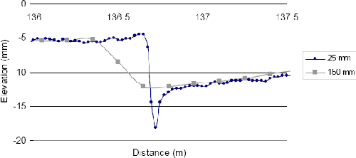
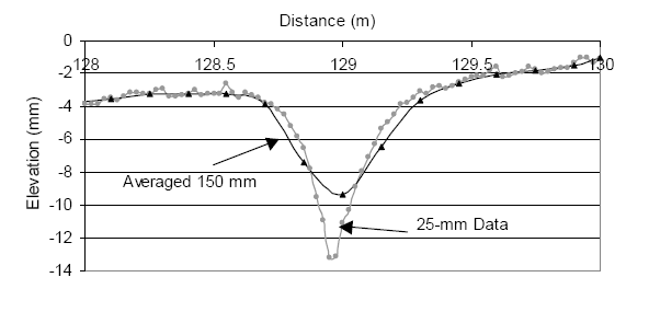
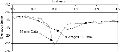
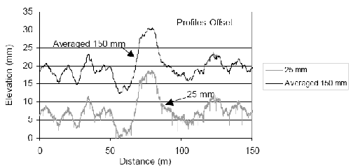
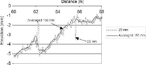
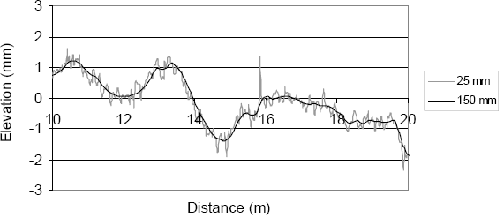
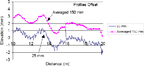
The regression equation indicated very good agreement in IRI between the two profilers. EFFECTS OF APPLYING A MOVING AVERAGE ONTO PROFILE DATAThe DNC 690 profilers collected profile data at 25.4-mm (1-inch) intervals and then applied a 304.8-mm (12-inch) moving average onto the data and recorded profile data at 152.4-mm (6- inch) intervals. Profile data collected at 25-mm (1-inch) intervals at LTPP test sections are available for both the T-6600 and ICC profilers. However, currently, in the LTPP program, these 25-mm (1-inch) profile data are processed using the ProQual software, which applies a 300-mm (11.8-inch) moving average onto the 25-mm (1-inch) profile data, and extracts profile data at 150-mm (5.9-inch) intervals. The IRI values for the LTPP sections are computed using this averaged data, and the averaged data are uploaded to the LTPP database. The application of the 300-mm (11.8-inch) moving average onto the 25-mm (1-inch) data attenuates very short-wavelength features that are present in the profile, and can also distort profile features that are actually present in the pavement. The averaged profile can show features that do not actually appear in the pavement, while not showing features that are actually present in the pavement. In this section, several examples that show the distortion caused in profile features by the application of the moving average are presented. Faulted PavementFigure 45 shows how the application of the moving average distorts the profile data collected over a fault. This figure shows the 25-mm (1-inch) interval data collected by the North Central T-6600 profiler over a faulted crack at the rough PCC section during the 1996 profiler verification study. The averaged data also are shown in this figure. The 25-mm (1-inch) data clearly define the fault, which is about 13 mm (0.5 inches). However, the application of the moving average makes the fault appear as a ramp, where there is a gradual change in elevation of about 7 mm (0.3 inches) that occurs over a distance of 0.3 m (1 ft). As seen in this example, the application of the moving average distorts the profile and shows a feature that does not actually exist on the pavement. 25.4 mm = 1 inch Figure 45. Profile distortion caused by the application of a moving average onto data collected over a fault. Effects of Downward FeaturesThe rough AC section that was used in the 2003 LTPP profiler comparison conducted in Minnesota had cracks that had been patched full width across the lane. Figure 46 shows the profile data obtained by the North Atlantic ICC profiler over such a patched crack. The figure shows the 25-mm (1-inch) data and the averaged data after the 25-mm (1-inch) data were processed using ProQual. The 25-mm (1-inch) data indicate that the patched crack is about 9 mm (0.4 inches) deeper than the adjacent pavement area. The application of the moving average onto the 25-mm (1-inch) data causes the depth of the patched crack to be reduced. 25.4 mm = 1 inch Figure 46. Profile distortion caused by the application of a moving average onto data collected over a patched crack. Figure 47 shows the 25-mm (1-inch) data and the averaged 150-mm (5.9-inch) interval data at the chip-seal section that was used in the 2003 LTPP profiler comparison. These data were collected by the North Atlantic ICC profiler. The 25-mm (1-inch) data show a crack that is at a distance of about 0.9 m (3 ft) as a sharp and narrow downward feature. However, the averaged data distorts the shape of the crack and makes the crack appear as a dip that is spread over a much wider length. The small variations between the profile data points that are seen in the 25-mm (1-inch) data are not seen in the averaged data. These variations are smoothed out by the application of the moving average. 25.4 mm = 1 inch Figure 47. Profile distortion caused by the application of a moving average onto data collected over a crack. Figure 48 shows profile data collected by the Western ICC profiler at site 3, which is a concrete section, during the 2003 profiler comparison in Minnesota. This figure shows both the 25-mm (1-inch) data and the averaged data after the 25-mm (1-inch) data were processed using ProQual. The 25-mm (1-inch) data clearly show the locations of the joints in the concrete pavement as downward spikes that occur at regular intervals. However, these features are not seen in the averaged profile because the averaging process attenuates the sharp downward features seen at the joints. 25.4 mm = 1 inch Figure 48. Application of a moving average onto data collected for a concrete pavement. Effects of Sharp Upward FeaturesFigure 49 shows a portion of the profile data collected by the North Central T-6600 profiler at section 3, which is a PCC section, during the 1996 regional verification test. The figure shows the 25-mm (1-inch) data and the averaged data after ProQual had processed the 25-mm (1-inch) data. The profile contains a sharp upward feature about 2.5 mm (0.1 inch) in height near 62 m (203 ft). The application of the moving average eliminates this feature. The application of a moving average onto a sharp upward feature that has a greater magnitude than the shown feature will cause the feature to appear in the averaged data as a feature that has a much lesser magnitude that is spread out over a much greater distance than the actual feature. The profile shown in figure 49 also shows a narrow downward feature between 65 and 66 m (213 and 216 ft). This feature also does not appear in the averaged data. Smooth Asphalt PavementFigure 50 shows a plot that contains profile data at 25-mm (1-inch) intervals, and the same data after it had been processed using ProQual. The profile shown in figure 50 contains data collected by the Western profiler along the left wheelpath at the smooth AC site during the 2003 LTPP profiler comparison. This pavement section is a smooth pavement, and there is no distress within the limits of the profile plot shown in figure 50. Both the 25-mm (1-inch) data and the averaged 150-mm (5.9-inch) data overlay well, except that the small spike seen at 16 m (52 ft) does not appear in the averaged data. 25.4 mm = 1 inch Figure 49. Application of a moving average onto a profile containing a sharp upward feature. 25.4 mm = 1 inch Figure 50. The 25-mm (1-inch) data and 150-mm (5.9-inch) averaged data from a smooth AC section. SUMMARY OF THE FINDINGSData recorded by inertial profilers do not accurately portray very narrow features such as cracks or joints in PCC pavements because of the low-pass filtering that is performed on the data. Evaluation of 25-mm (1-inch) data collected by both the T-6600 and ICC profilers over a joint in a PCC pavement showed that the joint appeared in the profile as a feature that was spread over a distance of 75 mm (3 inches), when the width of the joint was actually closer to 10 mm (0.4 inches). Although 25-mm (1-inch) interval data are collected by both the T-6600 and ICC profilers, the height sensors in the profilers collect data at much closer intervals and then average the data when computing profile data at 25-mm (1-inch) intervals. This causes the magnitude of a narrow feature that is recorded in the profile to be less than the actual magnitude, and also causes it to be spread out over a much wider distance than the actual feature. The application of an anti-aliasing filter onto the profile data can also have the same effect. 25.4 mm = 1 inch Figure 51. Offset profile plot of 25-mm (1-inch) data and averaged 150-mm (5.9-inch) data collected from a smooth AC pavement. Since the DNC 690 profiler recorded profile data at 152.4-mm (6-inch) intervals, when comparing data from the T-6600 profiler with the DNC 690 profiler, only the 150-mm (5.9-inch) interval ProQual-processed data from the T-6600 profiler can be used to perform a meaningful comparison. Comparison of the profile plots for the two profilers showed good agreement, although there were some differences between the profiles for sections that had significant longwavelength content. This difference is attributed to the different long-wavelength cutoff filter values used for the two profilers (91 m (300 ft) for the DNC 690 profiler and 100 m (328 ft) for the T-6600 profiler). An evaluation of the profile data indicated that the long-wavelength cutoff filtering technique used in both the DNC 690 and T-6600 profilers appears to be similar. There was very good agreement in IRI values for the DNC 690 and T-6600 profilers. Since 25-mm (1-inch) interval data were available for both the T-6600 and ICC profilers, a comparison of 25-mm (1-inch) interval data for the two profilers could be performed. Evaluation of the profile data using PSD plots indicated that there was good agreement in the profile data for the two profilers for wavelengths between 1 and 40 m (3 and 131 ft). For wavelengths less than 1 m (3 ft), the ICC profiler usually showed a higher wavelength content than the T-6600 profiler. This is attributed to the smaller footprint of the ICC profiler, which probably caused more texture effects and the higher magnitude of narrow features to be recorded. For wavelengths greater than 40 m (131 ft), the T-6600 profiler recorded more wavelength content than the ICC profiler. This is attributed to differences in the long-wavelength filtering techniques that are used by the two profilers. When ProQual-processed data for the two profilers were compared using a PSD plot, only the differences at the higher wavelengths will be seen, with good agreement being obtained between the two profilers for wavelengths less than 1 m (3 ft). This occurs because the application of the moving average attenuates the short-wavelength features. Good agreement in IRI, which is primarily influenced by wavelengths between 1 and 30 m (3 and 100 ft), was obtained for data collected by the ICC and T-6600 profilers. In the LTPP program, the 25-mm (1-inch) data obtained from the T-6600 and ICC profilers are processed using ProQual. ProQual applies a 300-mm (11.8-inch) moving average onto the 25-mm (1-inch) data and extracts data at 150-mm (5.9-inch) intervals, and these data are uploaded to the LTPP database. The application of the moving average onto the 25-mm (1-inch) data attenuates features with wavelengths less than 1 m (3 ft). Detailed profile features cannot be observed in the ProQual-processed data because of this effect. The moving average can also distort the profile data, with the averaged data showing features that are not actually present in the pavement, while eliminating features that are actually present.
|
|||||||||||||||||||||||||||||||||||||||||||||||||||||||||||||||||||||||||||||||||||||||||||||||||||||||||||||||||||||||||||||||||||||||||||||||||||||||||||||||||||||||||||||||||||||||||||||||||||||||||||||||||||||||||||||||||||||||||||||||||||||||||||||||||||||||||||||||||||||||||||||||||||||||||||||||||||||||||||||||||||||||||||||||||||||||||||||||||||||||||||||||||||||||||||||