LTPP Manual for Profile Measurements and Processing

CHAPTER 2. PROFILE MEASUREMENTS USING ICC PROFILER

2.1 INTRODUCTION

The ICC MDR 4086L3 profiler is a modified cargo van that is equipped with specialized instruments to measure and record road profile data. The MDR 4086L3 profiler contains three laser height sensors, an accelerometer located above each laser height sensor, a longitudinal distance measuring transducer, a computer system, signal conditioning electronics, and power control equipment. The three laser height sensors are mounted on a sensor bar that has been installed on the front of the vehicle. One sensor is located at the center of the vehicle, while the other two sensors are located along each wheel path. The longitudinal distance measuring transducer is mounted on the differential of the vehicle, and measures the distance traveled by the vehicle.

Laser height sensors measure the distance from the sensor to the road while the accelerometers measure vertical acceleration. Signals from the laser height sensors, accelerometers, and distance measuring instrument (DMI) are fed into a computer, which computes the profile of the pavement along the path traversed by each laser height sensor. Profiles along the paths traversed by the three sensors are displayed on the computer monitor during profile measurement. Data recorded by the height sensors, accelerometers, and DMI are stored in the hard disk of the computer. These data can be processed to obtain the profile along the path that was traversed by each sensor.

The profiler is also equipped with two photocells. One photocell is mounted vertically to sense reflections from pre placed marks on the road surface. The other photocell can be rotated around a horizontal axis, and can be positioned so it can sense reflections from pre placed cones with reflective markings that are placed on the side of the road. The photocell is used to perform a reference reset when it is triggered, and the location where it is triggered is stored in an event file. The profile vehicle is also equipped with both a heater and an air conditioner to provide a uniform temperature for the electronic equipment in the vehicle. According to ICC, the profiler can measure road profiles at speeds ranging from 10 to 112 km/h. The test speed normally used to profile LTPP sections is 80 km/h.

This section presents procedures that should be followed for collecting data with the ICC profiler. Most of the operating procedures that are specific to the equipment have been taken from the ICC Profiler Operation Manual.⁽¹⁾ This document and other ICC documents (see references 2, 3, 4, 5) should be consulted for additional details about the equipment and troubleshooting procedures.

2.2 OPERATIONAL GUIDELINES

2.2.1 General LTPP Procedures

2.2.1.1 Accidents

The operator shall inform the RSC as soon as possible after the mishap. Details of the accident should be reported in writing to the RSC. The corporate policy of the RSC should be followed in event of an accident. A police report of the accident should be obtained. Photographs showing damage to the vehicle should also be obtained.

2.2.1.2 Maintenance of Records

The operator is responsible for preparing and forwarding the forms and records to the RSC as described in section 2.8, which relate to testing and maintenance of the profiler.

2.2.1.3 Safety

Safety of the operators and traveling public is of great concern to LTPP, and safe driving and roadside practices are expected from LTPP operators.

2.2.1.4 Problem Reports

A profiler problem report (PROFPR) must be submitted whenever there are problems with equipment that affect the quality of data, data collection or data processing software, data collection guidelines, or any other problem related to profiling activities. The procedures described in appendix A must be followed when submitting a problem report.

2.2.2 Test Frequency and Priorities

Profile measurement frequency and priorities described in the latest applicable FHWA directive should be followed when profiling General Pavement Studies (GPS), Specific Pavement Studies (SPS), Seasonal Monitoring Program (SMP), and Weigh-in-Motion (WIM) sites.

2.2.3 General Operations

The following guidelines related to the operation of the profiler should be followed.

2.2.3.1 Laser Height Sensors

The profiler is equipped with three Selcom laser height sensors. The operator shall not let the laser beam strike his or her eye, as it can damage the eyesight. Furthermore, because it is not known if the reflection of the laser beam from a surface such as a polished base plate, a gauge block, or a watch can damage the eyesight, the operator shall take steps to avoid a reflected laser beam to come in contact with the eye. The FHWA will keep the RSCs informed of information on this safety issue as it becomes available. Always make sure that lasers are turned off when inspecting the sensor glass, cleaning the sensor, or performing maintenance on the sensors. The switch for turning the lasers on and off is located on the panel adjacent to the driver's seat (see figure 2.

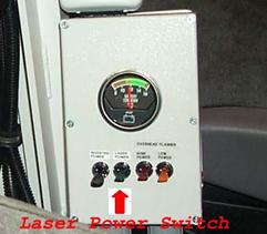
Figure 2. Photo. Laser on/off switch.

The Selcom laser height sensors in the profiler can malfunction at elevated temperatures. At approximately 50 °C the laser sensors will begin to produce errors, and at approximately 60 °C the laser sensors will turn off to prevent damage. Practical experience with the LTPP profilers has shown that the combination of ambient air temperature, radiant heat from the pavement, and internally generated heat of the laser sensors will cause the laser sensors to produce errors when the air temperature is approximately 39 °C. It is recommended that profiling be performed only when the air temperature is less than 38 °C. When it is necessary to schedule profile testing at sites where the air temperature is expected to exceed 38 °C, it should be anticipated that the testing may have to be scheduled for early morning or after-sunset hours.

2.2.3.2 Sensor Bar and Sensor Spacing

The sensor bar located in front of the vehicle is not designed to support the weight of the operator or other persons. Do not sit or stand on the sensor bar at any time. Sensors located along each wheel path should be at a distance of 838 mm from the center of the vehicle. This sensor setup results in a spacing of 1,676 mm between left and right sensors. The center sensor should be at the center of the vehicle, with the distance from left and right sensors to the center sensor being 838 mm.

2.2.3.3 Photocell Positioning

The profiler is equipped with two photocells. One photocell is mounted vertically to sense reflections from pre placed marks on the road surface. The other photocell can be rotated around a horizontal axis, and can be positioned so it can sense reflections from pre placed cones with reflective markings that are placed on the side of the road. The photocell is used to perform a reference reset when it is triggered, and the location where it is triggered is stored in an event file.

The two photocells in the profiler should be positioned such that the distance to the photocell from the edge of the right side of the profile sensor bar matches the distances shown in figure 3. The following sections give further details on the mounting of the horizontal and vertical photocell.

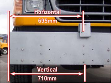
Figure 3. Photo. Locations of horizontal and vertical photocells.

2.2.3.3.1 Horizontal Photocell:

The horizontal photocell consists of a 90-degree mounting bracket that attaches to the top of the sensor bar and holds the photocell head (and cover plate) on a pivot bolt. This arrangement allows the photocell to be rotated up or down in order to detect the photocell target. The 90-degree bracket should be fastened to the sensor bar in its stock position, where the pivot bolt for the photocell is 695 mm from the right edge of the sensor bar. The mounting of the horizontal photocell is illustrated in figure 4.

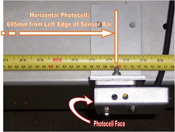
Figure 4. Photo. Position and mounting of horizontal photocell.

2.2.3.3.2 Vertical Photocell:

The vertical photocell consists of a 90-degree mounting bracket that holds the photocell vertically to a support bracket inside the profile sensor bar. The photocell bracket should be bolted to the right side of the sensor bar support bracket. The placement of the photocell bracket to the right side of the support bracket will center the photocell at 710 mm from the right side of the profile sensor bar. The photocell bracket can be mounted to elongated holes at the center of the support bracket (which centers the photocell front to back in the profile sensor bar). The photocell bracket should be adjusted so that the face of the photocell is approximately even with the underside of the profile sensor bar. Figure 5 illustrates the mounting and position of the vertical photocell from the underside of the profile sensor bar.

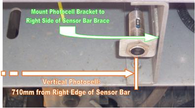
Figure 5. Photo. Position and mounting of vertical photocell.

2.2.3.4 Tire Pressure

The tire pressure should be checked prior to driving the vehicle in the morning to see if it is at the vehicle manufacturer's recommended values that are listed on the door and the fuel cover, which are 380 kPa (55 psi) for the front tires and 550 kPa (80 psi) for the rear tires (these are cold tire pressure values).

The tires should be sufficiently warmed up prior to testing. If the vehicle has traveled about 8 km at highway speeds after being parked, the tires are considered to have warmed up sufficiently. However, the distance for warming up tires may need to be changed depending on local weather conditions. Warming up the tires will cause a slight increase in the tire pressure (compared to cold tire pressure).

The DMI is affected by the tire pressure of the rear tires. The operator should have a copy of the Distance Calibration Report that was printed when the DMI of the profiler was last calibrated. This report will indicate the tire pressure of the rear tires during calibration. The tire pressure of the rear tires of the vehicle for all data collection runs should be within ±13.8 kPa (2 psi) of the tire pressure that was recorded when the DMI was last calibrated. Before performing a profile data collection run at a test section, the operator should adjust the tire pressure of the rear tires to ensure that the tire pressure is within this specified limit. The same tire pressure gauge should be used to measure tire pressure during both calibration and testing.

2.2.3.5 Major Repairs to Profile System Components

LTPP Major Maintenance/Repair Activity Report (see section 2.8.5) should be completed whenever repairs are performed on the profile system components such as the laser sensors, accelerometer, DMI, and data acquisition system. This report should also be completed if a laser sensor is replaced. DMI and accelerometers should be calibrated whenever repairs are performed on these components or the computer cards associated with these components. A full calibration check must be performed on the laser sensor when a laser sensor is replaced. A bounce test must be performed after a laser sensor or an accelerometer is replaced, when repairs are performed on the accelerometer, or when repairs are performed or replacements made to computer cards associated with these components.

After replacing a laser sensor, data collected by the profiler should be checked using the following procedure to ensure that accurate data are being collected:

1. Select a test section that has been profiled recently and is close to the current location of the profiler. When selecting the site, review comments that were made when the site was profiled to make sure that profile data available for this site is free of errors and that no unexplained spikes are present in the data. It is recommended that GPS-3 and SPS-2 sites be avoided, as significant variations in profile can occur on these sections due to temperature effects. The RSC should use his or her judgment in selecting an appropriate site to perform this comparison, taking into account the current location of the profiler and availability of a suitable site close to the location of the profiler.
2.  
3. Profile the selected site and obtain an acceptable set of runs as described in section 2.2.8.
4.  
5. Compare the profile data, as well as the IRI values, with the previously collected data for left and right sensors. If the repaired or replaced sensor is the center sensor, only the comparison of profiles can be performed, as IRI values for the center sensor cannot be computed. If evaluation indicates that the collected data is comparable with the previously collected data, the profile system components are considered to be functioning correctly.
6.  
7. Perform the comparison at another section if discrepancies are noted. If discrepancies are still noted, contact ICC to resolve the problem.
8.  

If a malfunction is detected in a sensor located along a wheel path, it may be replaced by the center sensor to continue data collection. The procedure to move a sensor is described in section 20 of the ICC Road Profiler Operations Manual.⁽¹⁾ (Warning: Each laser sensor is matched with a processing unit that is located at the back of the profiler. If a laser is switched (i.e., a wheel path sensor replaced by the center sensor) without the required changes in connection made to the processing unit, it will damage the laser. Such damages will not be covered by warranty. Therefore, operators should be aware that they need to clearly understand the procedure for switching a laser sensor and/or get technical assistance from ICC prior to switching a sensor.)

Once the repaired or replacement sensor is available, the center sensor that is now located at an outer position (left or right wheel path) should be moved back to the center position. A repaired or replaced sensor should be installed at the location of the defective sensor (either left or right wheel path). A full calibration check (see section 2.5.4) should be performed on the replacement sensor. Thereafter, the accelerometers should be calibrated (see section 2.5.3) and a bounce test (see section 2.3.3) should be performed. Procedures that were described previously (i.e., profiling at a previously profiled section) should be followed to ensure that the repaired or replaced sensor is functioning correctly.

2.2.3.6 Sensor Covers

The three laser sensors in the profiler are equipped with covers. Covers should be in place when testing is not being performed to protect the sensors. Covers should be taken off when performing sensor checks, performing bounce test, and collecting profile data.

2.2.3.7 Data from Previous Profile Visit

After collecting profile data at a site, the operator is required to compare the profile data, as well as IRI, with the data collected during the previous site visit as described in section 2.2.8. The profile data comparison between the visits is made using the Graphic Profiles feature in ProQual.⁽⁶⁾ Prior to setting out to profile a site, the operator must ensure that the data files that are required to do this comparison for the previous site visit are available. The operator should also have the IRI values for the site from the previous visits.

2.2.4 Computer System

2.2.4.1 Computer System in Profiler

The ICC profiler is equipped with two computers that are networked together. These two computer systems are referred to as system 1-Windows computer (Windows side), and system 2-DOS/MDR computer (DOS side).

Software for operating the profiler is located in system 2. This software is DOS based, and must be loaded from the DOS prompt. Data collected by the laser height sensor, accelerometer, and DMI during profiling are saved in system 2. System 1 contains Windows XP. The Windows based WinGraph software that displays a plot of the profile data while the data are being collected is located in system 1. The graphical plot of the profile created by WinGraph is saved in system 1.

There is a switch in the keyboard, video, and mouse (KVM) switch box that will switch the monitor between system 1 and system 2 (see figure 6). System 2 also has Windows 98 installed on it to enable sharing of the CD-ROM drive, Zip drive, and hard drive with the Windows XP system. System 2 must be in Windows 98 if it is to be accessed from system 1. Further details on use of the KVM switch to switch between the two systems during operation of the profiler will be presented in following sections of 2.2 and 2.3.

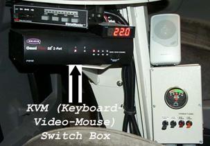
Figure 6. Photo. Keyboard, video, and mouse (KVM) switch.

Basic Input/Output System (BIOS) settings of system 1 and system 2 are described in the ICC Road Profiler Operation Manual.⁽¹⁾

2.2.4.2 Temperature Range for Computer Operation

Interior vehicle environment is critical to the operation of the onboard computers. The vehicle is equipped with a heater and an air conditioner to maintain interior temperatures within the required range. The interior of the vehicle should be between 10 and 35 °C before power is applied to the electronic equipment and the computer to protect them from damage. On cold days when the van has been parked outside, it can take up to 45 minutes to warm up the equipment inside the vehicle to 10 °C. If the interior temperature is below 10 °C, the computers will not boot up correctly. Even when the interior temperature in the van is greater than 10 °C, the computers may not boot up because the Uninterruptible Power Supply (UPS) that is located on the floor behind the driver's seat is at a temperature less than 10 °C. If such conditions are encountered, more time should be allowed for the interior of the vehicle to warm up.

2.2.4.3 Hardware and Software

The operator should maintain a copy of the ICC software and the ProQual software in the vehicle in case software problems occur in the software installed in the computer. If either of these software programs is reinstalled, the operator should go through the setup menus described in section 2.2.6 of this manual to make sure that appropriate parameters have been set to the correct values. ICC software programs that are installed in the profiler computer are the following:

• p90xfhwa.exe: Profiler runtime data collection program. This is a DOS program that is installed in system 2.
•  
• WinGraph.exe: Runtime graph program. This is a Windows program that is installed in system 1.
•  
• Winrp90l.exe: Report program and file converter. This is a Windows program that is installed in both systems 1 and 2.
•  
• FHWA_Eval.exe: Profile graphing, analysis, and IRI evaluation program. This is a Windows based program that is installed in both systems 1 and 2.
•  

Do not add any hardware (extra drives or other device) to the computer system before contacting ICC through the FHWA and its Technical Support Services Contractor (TSSC) to determine if they will interfere with the profile programs. Interference of profile programs due to additional devices may not be readily apparent.

Software supplied with the ICC profiler is tightly integrated. Other software installed into the computer can seriously degrade the performance and accuracy of the system. Apart from ProQual, other software should not be loaded onto the computer, unless specifically approved in writing by the FHWA.

Procedures for installing the ProQual program are described in the ProQual manual.⁽⁶⁾ ProQual may be installed in either system 1 or system 2. It has been reported by its developers that ProQual will run more efficiently in Windows XP, and printing of plots is much quicker when ProQual is run in Windows XP. If ProQual is installed in system 1, the data files should be copied from system 2 to system 1, and then processed by ProQual. Details on file copying procedures are presented in section 2.2.6.2

Profiler data files should be organized into subdirectories in the hard drive as outlined in LTPP directive GO-41 "Submission of Electronic Data for Customer Support and Ancillary Information Management System (AIMS)" (or current version of that directive).

2.2.5 Power Up, Booting, and Shutdown Procedures

2.2.5.1 Power Sources

There are two batteries in the profiler vehicle, one located under the hood of the vehicle (No. 1 battery), and one located in the rear right side of the vehicle (No. 2 battery). The rear battery supplies power to the computer and the electronic equipment in the profiler through an inverter. The computer and the electronic equipment in the profiler can also be powered through an external alternating current power source (house power). The rear battery should be charged when the profiler is connected to house power.

Both batteries in the profiler are charged when the vehicle engine is running. When the engine of the vehicle is not running, these batteries can be charged through a 15/2 fully automated battery charger connected to an external power source. In order to charge a battery when connected to an external power source, the House Power/Inverter Power switch (see figure 7) should be set to the "Inverter Power" position. The battery charger switches should be set to the 12 V and 10 AMP positions. The battery charger can be switched between No. 1 battery and No. 2 battery using the switch just below the House Power/Inverter Power switch (see figure 7). The battery charger has to be set to the battery that needs to be charged. The charger has automatic charge sensing capabilities that will not overcharge the battery.

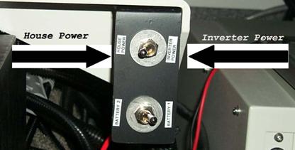
Figure 7. Photo. Power switch positions.

During data collection, power will be supplied through the inverter. When the engine is turned off (e.g., for monthly calibration check, troubleshooting, or operating computer when parked in office) an external power source can be used to supply power. The UPS in the van also makes it possible to switch from one power source to another (i.e., house power to inverter power) without having to shutdown the computer. The UPS will supply power to the system using its internal battery when making the switch. When the UPS is used without house or inverter power, the UPS battery is not being charged, and will drain down eventually to a point where it can no longer run the computers.

2.2.5.2 Switch Positions

The power switch in front of the inverter must always be left in the "Off" position (see figure 8).

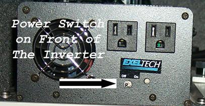
Figure 8. Photo. Inverter switch.

A remote switch located near the driver's seat controls the "On" and "Off" positions of the inverter. The No. 2 battery, which provides power for the MDR system (including inverter), is connected to the No. 1 battery and charges the system through a 70A continuous solenoid (with a diode to prevent voltage leakage) that is activated through a Ford van relay. This is a security feature to ensure that the No. 1 battery will not be drained if the remote inverter switch remains on when the vehicle is not running. If the remote inverter switch is accidentally left in the "On" position, the No. 2 battery will drain, and will have to be charged prior to operating the profiler. If the battery is not brought to a sufficient charge level prior to turning on the inverter, it is possible that the 70A continuous solenoid, that separates the No. 1 and 2 batteries, will burn out as the alternator attempts to bring the No. 2 battery to full charge. The laser power switch, inverter power switch, and computer power switch that are located on the computer case should always be kept in the "On" position (see figure 9). Power to these systems will be turned on or off from switches that are located near the driver's seat.

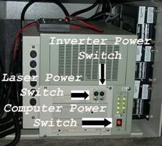
Figure 9. Photo. Switches on computer case.

2.2.5.3 Power-Up Procedure

Procedures for powering up the system using house power as well as inverter power are described in this section.

2.2.5.3.1 Power Up Using House Power:

1. Flip the power switch located in the back of the van to house power (see figure 7).
2.  
3. Make sure that the external 120 V power source is grounded. Plug the power cord into the port on the passenger side of the van.
4.  
5. Make sure the laser, inverter power, and computer power switches located on the computer case are in the "On" position (see figure 9).
6.  
7. Push the "On" button on UPS (see figure 10). The UPS is located behind the driver's seat.
8.  
9. Turn on the computer monitor (see figure 11).
10.  

2.2.5.3.2 Using Inverter Power:

1. Flip the power switch in the back of the van to inverter power (see figure 7).
2.  
3. Start the engine of the van.
4.  
5. Make sure the laser, inverter power, and computer power switches located on the computer case are in the "On" position (see figure 9).
6.  
7. Turn the power inverter on using the switch located on the panel below the monitor (see figure 12).
8.  
9. Push the "On" button on UPS (see figure 10).
10.  
11. Turn on the computer monitor (see figure 11).
12.  

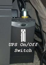
Figure 10. Photo. UPS on/off switch.

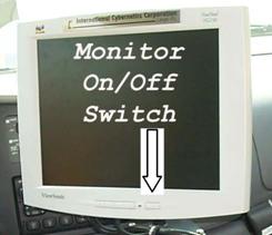
Figure 11. Photo. Monitor on/off switch.

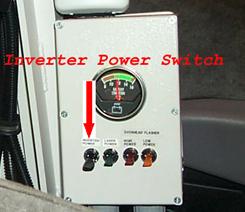
Figure 12. Photo. Remote switch for inverter power.

2.2.5.4 Computer Booting Procedure

Follow the instructions below to complete the computer booting procedure:

1. Supply power to the system using either house power or inverter power as described in section 2.2.5.3.
2.  
3. Allow the computer to come up to the Login screen for Windows XP. Login using LTPP as the user name and LTPP as the password. The monitor will show that Windows XP is running.
4.  
5. Double click the ICC icon for WinGraph if the computer system is powered up to collect profile data or to perform the bounce test, else go to step 4. If the WinGraph icon is double clicked, WinGraph will run on system 1.
6.  
7. Switch the KVM to system 2 (see figure 6).
8.  
9. Allow the DOS-MDR system to proceed to the DOS prompt.
10.  
11. Check the date and time on system 2 and adjust to correct local time, if needed.
12.  
13. Type m and then press the Enter key at the c:\ prompt to run the MDR data collection program. The main menu of the MDR program should now be shown on the computer monitor (see figure 13).
14.  

Figure 13. Screen shot. MDR main menu (1).

The MS-DOS commands Date and Time should be placed in the AUTOEXEC.BAT file in system 2 so that when the computer is turned on it will prompt the operator for date and time. This will ensure that data files have the correct date and time stamp. Time should correspond to that of the time zone where the section is located. When the computer prompts for date and time, the operator should check if current values are correct. If they are correct, the operator can press the Enter key at each prompt. If they are incorrect, correct values should be entered.

2.2.5.5 Shutdown Procedure

Follow the instructions below to complete the shutdown procedure:

1. Remove the CD-ROM if it is present in a drive and remove any flash drives that are attached to the computer.
2.  
3. Turn off power to the lasers by flipping the switch on the monitor stand (see figure 2) to the down position.
4.  
5. Use the KVM switch (see figure 6) to go to system 2 if the monitor shows that the computer is not in system 2. System 2 could be either in Windows 98 or in the MDR program.
6.  
7. Select Quit from main menu, and then enter Y to confirm the quit request if the MDR program is running. The C:\ prompt will then be displayed on the screen. If the system is in Windows 98, exit all programs, select the "Start" button at the bottom left hand side of the screen, select "Shutdown," and then indicate you want to shutdown the system. Wait until the screen says "Its now safe to turn off your computer."
8.  
9. Use the KVM switch (see figure 6) to get to system 1.
10.  
11. Exit all programs, select the "Start" button at the bottom left hand side of the screen, and select "Turn Off Computer." Confirm the request to turn off the computer. Wait until the screen says "Its now safe to turn off you computer."
12.  
13. Turn off the UPS located behind the drivers seat (see figure 10). The power to the computers will now been turned off.
14.  
15. Unplug the house power input from the profiler if shutting down when the system is being powered by house power. If shutting down when being powered by the vehicle (through the inverter), turn off power inverter by flipping the switch on the monitor stand to the down position (see figure 12).
16.  

2.2.6 Software Setup Parameters

The MDR software is used to collect and save profile data. Collected profile data is processed using the ProQual software. Most settings in the MDR program were set at appropriate values when the software was installed in the profiler. However, these settings need to be checked to make sure they are correct, and if incorrect, necessary corrections must be made. These settings should be checked if the software is reinstalled in the computer or if problems are encountered with software. There are some fields in ProQual that have to be set by the user once the software is installed. Settings in the MDR program and ProQual program that need to be checked and/or updated are presented in sections 2.2.6.1 and 2.2.6.2, respectively.

2.2.6.1 Settings in MDR Software

The settings in the MDR software should be checked to ensure that they are set at correct values. There are some settings that the user will have to set or update once the software is installed. These settings are specific to the data collected for the LTPP program. The following steps take the operator through the different settings that need to be checked and/or updated:

1. Follow the procedures described in section 2.2.5.4 to launch the MDR software, omitting step 3. MDR main menu should now be displayed on the screen (see figure 13).
2.  
3. Select "Options" in the MDR main menu and the drop down menu shown in figure 14 will be displayed on the monitor. The Reference Post Display Mode should show "Meter," the User should show "LTPP," and the Version should correspond to that shown in figure 14. If any of these fields are different, reset the values to the previously described values.
4.  
5. Highlight "ICC System Parameters" in the Options Menu (see figure 14) and press the Enter key. The screen shown in figure 15 will be displayed.
   

   
   Figure 14. Screen shot. Options menu (1).

   
   Figure 15. Screen shot. ICC system parameters screen.

   The parameter settings should match the following values (Note: Parameter settings for Target may be different depending on the photocell that will be used for testing).

   Parameter settings that are shown in figure 15 are as follows, and the parameter settings shown in the monitor should match these values (except for four and five of the Target, which may have a different value).

   Profile Sensors Com2 Mode 1 Com1 Port Setup 3F8h 9600 E3h Com1 3 LCD Port Setup 4 Cmd Port Setup MDR Prog Files Dir Report List Accelerometer Filter delay (-ms)

   1 2 3 Off 2F8h 9600 E3h Com2 On 3F8h 9600 83h Com1 On C:\MDRSW\ C:\MDRSW\MDRRPT.LST -5

   If any of the parameters shown on the monitor are different, reset the parameters so they correspond to the previously described values.

   Target one, two, and three should show NA. Target four and five will show the photocell that has been selected. Refer to step 3 in section 2.3.4.1 on how to select photocells.

   After the parameter settings have been checked, press Escape key twice to get back to the MDR main menu (see figure 13).

6.  
7. Select "Calibration" in the main menu and the drop down menu shown in figure 16 will be displayed. Highlight "Sensors" in this menu, and press the Enter key. The Sensor Calibration menu shown in figure 17 will be displayed on the monitor.

   
   Figure 16. Screen shot. Calibration menu (1).

   
   Figure 17. Screen shot. Sensor calibration menu (1).

   In this menu, highlight "Sensor Config" and press the Enter key. The sensor configurations will be displayed on the monitor (see figure 18).

   
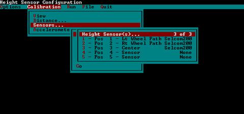
   Figure 18. Screen shot. Sensor configurations.

   The parameter settings shown on the monitor should match the values shown in figure 18, which are the following:

   Height Sensor(s)... 3 of 3

   1 - Pos	1 - Lt Wheel Path	Selcom200
   2 - Pos	2 - Rt Wheel Path	Selcom200
   3 - Pos	3 - Center	Selcom200
   4 - Pos	4 - Sensor	None
   5 - Pos	5 - Sensor	None

   If the parameters shown on monitor are different, reset the parameters so they correspond to the previously described values. After checking the values of the parameters, press the Escape key to get to the Sensor Calibration menu.

8.  
9. Highlight "Spacing" in the Sensor Calibration Menu (see figure 17) and press the Enter key. This will bring up the Sensor Spacing submenu that has three choices: Key Rut Positions, Rutting Order, and Spacing (see figure 19).

   
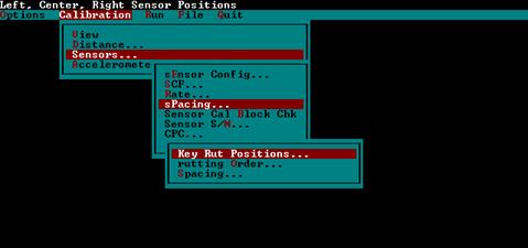
   Figure 19. Screen shot. Sensor spacing submenu.

   Highlight "Key Rut Positions" and press the Enter key. The Key Rut Positions screen shown in figure 20 will be displayed on the monitor. Values shown on the monitor should match the values shown in figure 20, which are:

   1 - Left Pos	1
   2 - Center Pos	3
   3 - Right Pos	2

   
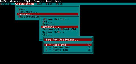
   Figure 20. Screen shot. Key rut positions screen.

   If any of the parameters are different, reset the parameters to the values that were indicated. After checking the parameters, press the Escape key to get back to the Sensor Spacing submenu (see figure 19).

10.  
11. Highlight "Rutting Order" in the Sensor Spacing submenu (see figure 19) and press the Enter key. The monitor will show the Rutting Order screen shown in figure 21. Values for the parameters shown on the monitor should match the values shown in figure 21, which are the following:
    

    1 -	Sensor Pos # 1
    2 -	Sensor Pos # 3
    3 -	Sensor Pos # 2
    4 -	Sensor Pos # 0
    5 -	Sensor Pos # 0

    
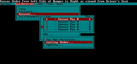
    Figure 21. Screen shot. Rutting order screen.

    If any of the parameters are different, reset the parameters to the indicated values. After checking the parameters, press the Escape key to get back to Sensor Spacing submenu (see figure 19).

12.  
13. Highlight "Spacing" in the Sensor Spacing submenu and press the Enter key. The monitor will show the sensor spacing screen shown in figure 22.

    
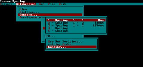
    Figure 22. Screen shot. Sensor spacing screen.

    The values displayed on the monitor should be identical to the values shown in figure 22, which are the following:

    1 - Spacing	1 - 1 0 mm
    2 - Spacing	1 - 3 838 mm
    3 - Spacing	1 - 2 1676 mm
    4 - Spacing

    If any of the parameters are different, set the parameters to the indicated values by highlighting the parameter, pressing the Enter key, entering the correct value in the window that opens, and pressing the Enter key again to close the window. After checking the parameters, press the Escape key twice to get back to the Sensor Calibration Menu (see figure 17).

14.  
15. Highlight "Sensor S/N" in the Sensor Calibration Menu (see figure 17) and press the Enter key. The Sensor Serial Number screen shown in figure 23, which shows the serial numbers of the sensors, will be displayed.

    
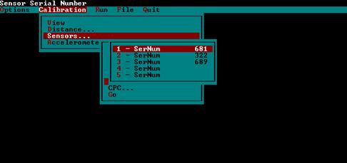
    Figure 23. Screen shot. Sensor serial number screen.

    The serial numbers shown on the monitor will be different from those shown in figure 23. Check to see if the serial numbers displayed match the serial numbers of the lasers in the profiler. In the profiler, position one is the left wheel path, position two is the right wheel path, and position three is the center sensor. The laser sensor serial numbers are marked on the front of each laser's processor unit, which is located to the right of the computer chassis. If the displayed serial numbers are not correct, highlight the appropriate sensor, press the Enter key, type the correct serial number in the window that opens, and press the Enter key again to close the window. When done, press the Escape key three times to get to the MDR main menu (see figure 13).

16.  
17. Select "Run" in the MDR main menu (see figure 13) and the Run Menu shown in figure 24 will be displayed on the monitor.

    
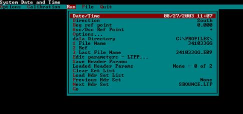
    Figure 24. Screen shot. Run menu (1).

    Select "Options" in this menu and the Run Options menu shown in figure 25 will be displayed on the monitor.

    
    Figure 25. Screen shot. Run options menu (1).

    The values for parameters shown on the monitor should match the values shown in figure 25, which are the following:

    HW DMI Simulator	Off
    SW DMI Simulator	Off
    User mode	SINGLE
    Profile	On
    Graph Profile	On
    LCD Display	Com1 On 1
    Speed Collect	On
    Speed Limit	+1.6
    Target	Com1 On/Com2 Off
    Command Mode	Com2 On
    IRI	On

    If the value shown on the monitor for Speed Limit is different, highlight Speed Limit and press the Enter key. Next, type 1.6 in the window that opens and press the Enter key to close the window. The HW DMI Simulator should indicate "On" only when the bounce test is performed, and should indicate "Off," as shown in the figure, at other times. If the DMI Simulator indicates "On," highlight the DMI Simulator and press the Enter key to make it "Off." If the values shown for any of the other parameters are different, reset the parameters to the values that were indicated previously.

18.  
19. Select "IRI..." in the Run Options Menu (see figure 25) and the IRI Options screen shown in figure 26 will be displayed on the monitor.

    
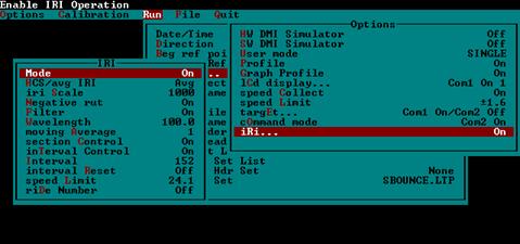
    Figure 26. Screen shot. IRI options screen (1).

    The values of the parameters shown on the monitor should match the values shown in figure 26, which are the following:

    Mode	On
    HCS/Avg IRI	Avg
    iri Scale	1000
    Negative rut	On
    Filter	On
    Wavelength	100.0
    moving Average	1
    section control	On
    interval Control	On
    Interval	152
    interval Reset	Off
    speed Limit	24.1
    ride Number	Off

    Highlight "Interval," press the Enter key and check if the value shown in the box that opens up is 152.4. If not, edit the value so that it is set to 152.4, and press the Enter key to close the window. If Speed Limit does not show a value of 24.1, highlight Speed Limit, press the Enter key, type 24.1 in the window that opens, and press the Enter key to close the window (value for Speed Limit represents the speed below which data will not be included in the file). If any of the other parameters shown on the monitor are different from the values shown on figure 26, reset the parameter to the appropriate value. After checking the parameters, press the Escape key three times to get back to the MDR main menu.

20.  

2.2.6.2 Settings in ProQual Software

As indicated in section 2.2.4.3, ProQual may be installed in either system 1 or system 2. If ProQual is installed in system 1, the data files should be copied from system 2 to system 1, and then processed by ProQual. In order for files to be copied from system 2 to system 1, system 2 must be booted in Windows 98. Use the following procedure to copy files from system 2 to system 1:

1. Switch to the Windows XP computer.
2.  
3. Explore the "C on DOS/Windows (G:)" disk drive.
4.  
5. Copy the raw profile data folder (folder containing files with extensions p, v, and e) to a known location on the Windows XP hard disk drive (C drive).
6.  
7. Run ProQual and select the files with extension p on the Windows XP hard disk (C drive) to load the data files when processing files.
8.  

After ProQual is installed, there are several parameter settings that have to be entered (or set) and others that have to be checked. Use the following procedure to set/check the parameter settings:

1. Start ProQual and then select System to bring up the System menu shown in figure 27.

   
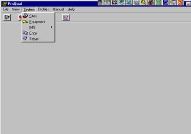
   Figure 27. Screen shot. ProQual system menu.

2.  
3. Select "Equipment" and the monitor will display a screen similar to that shown in figure 28. Entries for Serial # and photocell offsets displayed on the monitor will be different from the values shown in figure 28.

   
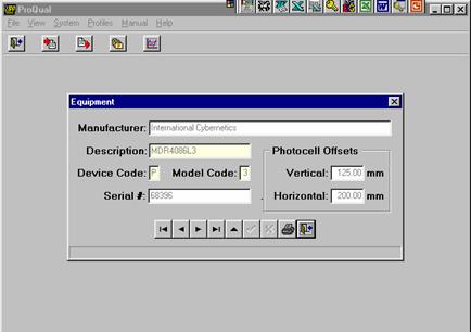
   Figure 28. Screen shot. Equipment screen in ProQual.

4.  
5. Check the Serial Number and Photocell Offsets. Adjust the settings if needed for serial number and photocell offsets using following procedure:
   1. Use the second button from the left at the bottom (prior equipment record) or third button from the left (next equipment record) to scroll through screens until the Serial Number matches last five digits of the VIN number of profiler. (Note: when the mouse is on a button, a message will appear at the bottom of screen that describes the function of that button). The Manufacturer field should now show "International Cybernetics."
   2.  
   3. Check to see if the vertical and horizontal photocell offsets shown match the offset values for the profiler. These photocell offsets values for the profiler are determined annually using the procedure described in section 2.6.3. If the photocell offset values shown are not correct, click the fifth button from left at the bottom of the screen (edit equipment report). This will allow the values shown for photocell offsets to be edited. Use the mouse to click on the appropriate offset field(s) and type the correct offset value(s). Click on the sixth button from the left (save equipment changes) to save the changes.
   4.  
   5. Click on the rightmost button at the bottom of the screen to exit s to the main menu.
   6.  
6.  
7. Select Setup in the Systems menu (see figure 27). The Analysis Parameters screen shown in figure 29 will then be displayed on the monitor.

   
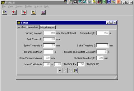
   Figure 29. Screen shot. Analysis parameter screen in ProQual.

   The value for each parameter should exactly match the values shown in figure 29. These values are set to the correct value when ProQual is installed. It is possible to edit these values using the first button at the bottom of screen. However, the operator should never edit any of the values shown on this screen, unless directed by the project engineer.

   The following parameters shown in figure 29 are not currently used in any computations: Sample Length, Fault Threshold, and RMSVA Base length. The other parameters are used in computations, and a brief description of each of these parameters follows:

   • Running Average: This is the interval at which profile data is output in ProQual.
   •  
   • Spike Threshold 1: Threshold for double elevation spikes.
   •  
   • Spike Threshold 2: Single elevation spike threshold.
   •  
   • Tolerance on mean: Tolerance on mean IRI that is used to determine if IRI of a set of profile runs is acceptable.
   •  
   • Tolerance on standard deviation: Tolerance on standard deviation of IRI that is used to determine if a set of profile runs is acceptable.
   •  
   • Slope Variance Interval: Base length used to compute slope variance.
   •  
   • Mays Coefficients: Coefficients used to compute the Mays Coefficient.
   •  
8.  

2.2.7 Field Operations

2.2.7.1 Turnarounds

Applicable laws in each State regarding use of median turnarounds must be followed.

2.2.7.2 Strobe Bar, Flashing Signal Bar, and Signs

The profiler is equipped with a strobe bar in front and a flashing signal bar in the rear. Both the strobe bar and flashing signal bar should be turned on during testing. In addition, the magnetic sign "Caution Road Test" should be mounted at the back of the vehicle during testing. This sign should be taken off when traveling between sites to alleviate any confusion that may be perceived by other road users.

2.2.7.3 File Naming Convention

The file naming convention to be used in specifying the name of data file in the LTPP Menu of the profiler software (see section 2.3.4.1) for GPS, SPS, and SMP sections are described in this section (for file naming conventions for WIM sites, refer to section 2.4.2.3). Failure to adhere to the file naming convention could produce errors when running ProQual, and will cause problems when archiving files. The file name should consist of eight characters as follows:

1. Characters one and two: State code of the State in which the site is located (e.g., 27 for Minnesota).
2.  
3. Characters three to six: Four-digit site number. For GPS and SMP sites, this is the four-digit LTPP identification number (e.g., 1023). For SPS sites, the third character should be zero, A, B, etc., depending on project code (e.g., 0300, A300, B300, etc.). The fourth character for SPS sites is the experiment number (e.g., 2 for SPS-2 projects), while the fifth and sixth characters should be zero. However, if an RSC elects to do so, for SPS sites it is permissible to use the fifth and sixth character to indicate the first section encountered when the SPS section is profiled.
4.  
5. Character seven: Letter code defining section type. This is G for GPS, S for SPS, M for SMP or C for Calibration test sections.
6.  
7. Character eight: Sequential visit identifier code that indicates the visit code for the current profile data collection. This identifier indicates the number of times a set of profile runs has been collected at a site since the site was first profiled with the K. J. Law T-6600 profiler. When the site was first profiled with the K. J. Law T-6600 profiler, the letter A was used for the eighth character. Use an appropriate letter for the current profiling. For example, if the site is being profiled for second time use letter B, use C for the third time, H for eighth time and so on. For rigid pavement test sections in the SMP, a different character shall be used each time a set of profiles is obtained during the day. If a site is being profiled for the first time (it has not been profiled by K. J. Law profiler before, as is the case for some GPS-6B or GPS-7B sites), the letter A should be used for the eighth character. Thereafter, this letter should be sequentially increased (B, C, and so on) during subsequent profile data collection visits. If a region has been using the sequential visit identifier to indicate the number of times a set of profiles has been obtained at the site since its inception into the LTPP program, that procedure is also acceptable. In such case, the letter A is used to denote the first time the site was or is profiled by the RSC, whether with the DNC690, T-6600 or the ICC profiler. Thereafter, this letter should be sequentially increased (B, C, and so on) during subsequent profile data collection visits.
8.  

After the sequential visit identifier code has been assigned as Z, use the following procedure for file naming when the site is profiled the next time:

1. If the site is a SMP site, change character seven to N, and assign the site visit identifier to be A. For subsequent profile visits, maintain character seven as N and change the sequential visit identifier to be B, C, D, etc.
2.  
3. If the site is a GPS site, change character seven to H, and assign the site visit identifier to be A. For subsequent profile visits, maintain character seven as H and change the sequential visit identifier to be B, C, D, etc.
4.  
5. If the site is a SPS site, change character seven to T, and assign the site visit identifier to be A. For subsequent profile visits, maintain character seven as T and change the sequential visit identifier to be B, C, D, etc.
6.  

The following are examples of valid data file names:

• 171002GD: GPS section 1002 in Illinois (State code = 17), profiled for the fourth time.
•  
• 260200SB: SPS-2 site in Michigan (State code = 26), profiled for the second time.
•  
• 271018MB: Seasonal monitoring site 1018 in Minnesota (State code = 27), profiled for second time.
•  
• 27A300SC: SPS-3 sites having project code A in Minnesota (State code = 27), profiled for the third time.
•  

If a long SPS project is not profiled continuously, but profiled in groups of sections, the sixth character in the file name should be replaced by a character for each group. For example, consider the SPS-2 project in State 26 that is profiled as two groups of sections. The file name for the first group could be 26020ASA, while that for the second group could be 26020BSA.

The first two digits of the file name for a section must be valid State codes when generating file names for demonstration purposes or comparative studies. ProQual will not operate on data files that do not follow this convention.

2.2.7.4 Operating Speed

A constant vehicle speed of 80 km/h should be maintained during a profile measurement run. If the maximum constant speed attainable is less than 80 km/h due to either traffic congestion or safety constraints, then a lower speed should be selected depending on prevailing conditions. If the speed limit at the site is less than 80 km/h, the site should be profiled at the posted speed limit. If traffic traveling at high speeds is encountered at a test site, it is permissible to increase the profiling speed to 88 km/h. If a site is relatively flat, cruise control should be used to maintain a uniform speed. It is important to avoid changes in speed during a profile run that may jerk the vehicle or cause it to pitch on its suspension. A change in throttle pressure or the use of brakes to correct vehicle speed should be applied slowly and smoothly.

2.2.7.5 Event Initiation

During profile data collection, the data collection program uses an event mark to record a Reference Reset in the event file. Event marks are generated by the photocell. The vertical photocell detects the white paint stripe or reflective tape at the beginning of the test section and sends a signal to record that event in the event file. This information is used to generate the data corresponding to the test section. In those instances in which existing paint mark on pavement is not able to trigger the vertical photocell, the horizontal photocell should be used. A cone with a reflective marker or an FHWA approved device should be placed on the shoulder at the beginning of the test section to activate the horizontal photocell. The leave edge of the reflective marker should be aligned with the leave edge of the stripe at the beginning of the test section.

2.2.7.6 Loading and Saving Files

Saving files to the hard disk, flash drive, zip disk or floppy disk, or loading files from the hard disk, flash drive, zip disk, floppy disk or CD ROM should not be done when the vehicle is in motion. At the completion of a profile run, driver should pull over to a safe location and come to a complete stop, enter end of run comment, and then save data file to a hard disk.

2.2.7.7 Inclement Weather and Other Interference

Inclement weather conditions (e.g., rain, snow, heavy cross winds) can interfere with the acquisition of acceptable profile data. Profile measurements should only be performed on dry pavements. In some cases, it may be possible to perform measurements on a damp pavement with no visible accumulation of surface water. Under such circumstances, the data should be monitored closely for run to run variations and potential data spikes. ProQual should be used to detect spikes. This program uses a threshold value of 5 mm to identify single elevation spikes. When reviewing data, the operator should keep in mind that spikes could occur due to pavement conditions (e.g., potholes, transverse cracks, bumps), and electronic interferences.

Changing reflectivity on a drying pavement due to differences in brightness of pavement (light and dark areas) may yield results inconsistent with data collected on uniformly colored (dry) pavements. Run to run variations in data collected under such conditions should be carefully evaluated. If problems are suspected, profile measurements should be suspended until pavement is completely dry.

Electromagnetic radiation from radar or radio transmitters may affect data recorded by the profiler. If this occurs, the operator should attempt to identify and to contact the source to learn if a time will be available when the source is turned off. If such a time is not available, it may be necessary to schedule a Dipstick^® survey of the test section.

2.2.7.8 End of Run and Operator Comments

The profiler software allows the operator to enter comments at the end of each profile run, and those comments are hereafter referred to as end of run comments. If required, these comments can be edited in ProQual when the data files are imported. The operator can also enter comments about the profiled site after profile data is imported to ProQual and those comments are hereafter referred to as operator comments. Both sets of comments can be up to 55 characters in length and are uploaded into the LTPP PPDB. Examples are provided in this section separately for end of run comments and operator comments with the suggested format for the comment.

2.2.7.8.1 End of Run Comments:

End of run comments entered for a group of sections profiled in one run (e.g., SPS site) are put into an individual file that is subsectioned from that profile run. Similarly, if a GPS section is profiled in conjunction with a SPS site in one run, end of run comments are common to all sections subsectioned from that profile run. Therefore, the operator should ensure that end of run comments that are entered when several test sections are profiled in one run are valid or applicable to all sections in that run (e.g., weather related comment). End of run comments should be typed in capital letters.

To ensure uniformity between the end of run comment that is made when a group of sections are profiled together (e.g., SPS section) and when a section is profiled as an individual section (e.g., GPS section), end of run comments have been grouped into the following three categories:

• Good Profile Run: Comment used to indicate that the profile run was good and that no problems were encountered. Example comment: RUN OK.
•  
• Environment Related Comments: Profile testing should not be performed when environmental conditions are such that they can affect the quality of the data. If the operator believes there is a possibility that environmental conditions may have affected the quality of the data, a comment should be entered.
  Example comment: HEAVY WINDS.
•  
• Speed Related Comments: The following are examples where a comment related to speed of testing should be entered:
  • Speed limit at site is lower than the 80 km/h specified for profile data collection.
    Example comment: SPEED LIMIT AT SITE IS 60 KM/H.
  •  
  • Heavy traffic makes it difficult to maintain a constant speed.
    Example comment: TRAFFIC CONGESTION: SPEED VARIABLE.
  •  
  • Grade (uphill or downhill) makes it difficult to maintain constant speed.
    Example comment: DIFFICULT TO MAINTAIN CONSTANT SPEED: UPGRADE.
  •  
•  

End of run comments are made at end of the run prior to saving the data. ICC software offers six end of run comments that the user can select at the end of a run. If none of these comments are applicable, the user can type any desired comment. The six end of run comment options that are available in the ICC software are as follows:

• RUN OK.
•  
• PAVEMENT SURFACE DAMP.
•  
• TRAFFIC CONGESTION SPEED VARIABLE.
•  
• DIFFICULT TO MAINTAIN CONSTANT SPEED: UPGRADE.
•  
• DIFFICULT TO MAINTAIN WHEEL PATH LOCATION.
•  
• LATE PHOTOCELL INITIATION.
•  

There should always be an end of run comment. If no problems were encountered during the run, the comment "RUN OK" should be entered as an end of run comment. If there were weather/environmental related comments, or speed related comments, these should be entered following the guidelines that were presented previously. If a late photocell initiation is suspected, an additional run to replace that run should be obtained.

2.2.7.8.2 Operator Comments:

Operator comments are entered after profile data has been imported into ProQual and reviewed. Operator comments should be typed in capital letters. They can fall into one of the following six categories:

1. Pavement Distress Related Comment: A comment should be made if there are pavement distresses or features within the section that can affect the repeatability of profile data. Comment should specify the distress(es) present that the operator believes to be causing non-repeatability of profile data. The following are examples where such comments may be entered:
   1. For AC pavements, distresses such as rutting, fatigue/alligator cracking, potholes, patches, longitudinal and transverse cracking.
      Example comment: _________ IN SECTION (enter distress type for blank).
   2.  
   3. For concrete pavements, distresses such as faulting, spalling, longitudinal and transverse cracking
      Example comment: _________ IN SECTION (enter distress type for blank).
   4.  
   5. For pavements with a chip seal, a comment should be entered if chips are missing in areas within the section.
      Example comment: CHIP SEAL SECTION. CHIPS MISSING.
   6.  
   7. For sections with dips, comment should be made if there are dips within the section.
      Example comment: DIPS IN SECTION.
   8.  
2.  
3. Maintenance Related Comments: A comment should be made if the operator is familiar with the test section and notes that recent maintenance and/or rehabilitation activities (e.g., overlays, patches, crack filling, or aggregate seals) have been performed on that section. The operator should specifically make a note if overband type crack filling has been performed on the section.
   Example comment: RECENT MAINTENANCE IN SECTION, PATCHES.
4.  
5. Wheel path Tracking Related Comments: A comment should be entered if the operator encountered problems in tracking the wheel path. Such comment should be entered if one or more of the following conditions are encountered:
   1. During profile run, path followed was either to the left or to right of wheel path.
      Example comment: RUN RIGHT OF WHEEL PATH.
   2.  
   3. Difficulty in holding wheel path due to pavement distress(es) such as rutting.
      Example comment: DIFFICULT TO HOLD WHEEL PATH, RUTTING.
   4.  
   5. Difficulty in holding wheel path due to truck traffic.
      Example comment: DIFFICULT TO HOLD WHEEL PATH, TRAFFIC.
   6.  
   7. Difficulty in holding wheel path due to wind.
      Example comment: DIFFICULT TO HOLD WHEEL PATH, WINDY.
   8.  
   9. Difficulty in holding wheel path because of grade, either uphill or downhill.
      Example comment: DIFFICULT TO HOLD WHEEL PATH, UPHILL.
   10.  
   11. Difficulty in holding wheel path because section is on a curve.
       Example comment: DIFFICULT TO HOLD WHEEL PATH, CURVE.
   12.  
6.  
7. Location of Test Section Comments: A comment should be entered if the location of a section has a potential impact on obtaining repeatable profile runs. Such conditions include the following:
   1. Section or approach to section is on a curve.
      Example comment: APPROACH TO SECTION ON CURVE.
   2.  
   3. Section or approach to section is on a grade (uphill or downhill).
      Example comment: SECTION ON A DOWNHILL.
   4.  
8.  
9. Miscellaneous Other Comments: A comment should be entered if conditions other than those not covered previously are encountered during profiling that may affect quality of the data. Such conditions include the following:
   1. Contaminants on road such as sand/gravel or dead animals.
      Example comment: SAND ON ROAD.
   2.  
   3. Traffic or WIM loops within test section.
      Example comment: WIM LOOPS WITHIN SECTION OR TRAFFIC LOOPS IN SECTION.
   4.  
   5. Color variability of the pavement because of salt application.
      Example comment: COLOR VARIABILITY CAUSED BY SALT.
   6.  
   7. Excessive vehicle movements just prior to test section because of pavement condition.
      Example comment: CORE HOLES ON WHEEL PATH BEFORE SECTION.
   8.  
10.  
11. Spike Related Comments: After ProQual has processed the data, the operator should look for presence of spikes in the data. If spikes are present, enter comment indicating whether or not the spikes are pavement related.
    Example comment: PAVEMENT RELATED SPIKES IN PROFILE.
12.  

After data is processed using ProQual, an operator comment can be entered for each run by going to the Run Details Tab in ProQual. ProQual offers six comments that can be selected by the operator. These comments are the following:

• EQUIPMENT OK.
•  
• ROUGH SURFACE TEXTURE / RAVEL & STONE LOSS.
•  
• MODERATE TO SEVERE SURFACE FLUSHING.
•  
• NOTICEABLE DISTRESS IN WHEEL PATH.
•  
• MODERATE TO SEVERE RUTTING.
•  
• FAULTING AND SPALLING OF JOINTS / CRACKS.
•  

The operator also has the option of typing any desired comment. The operator can also select one of the default comments available in ProQual, and type an additional comment at the end of the selected comment.

Operator comments can be up to 55 characters in length. If spikes are observed in the profile, it is mandatory for the operator to enter a comment regarding these spikes after running ProQual to indicate whether or not the spikes are pavement related. Because of the 55 character constraint, it may not be possible to type in all of the applicable factors from the list of factors that were described previously. Therefore, when entering comments, it is recommended that the following order of priority (with the first factor listed being given the highest priority) be followed:

1. Wheel path tracking related comments.
2.  
3. Pavement distress related comments.
4.  
5. Maintenance related comments.
6.  
7. Miscellaneous other comments.
8.  
9. Location of test section comments.
10.  

It should be noted that comments are used to indicate factors that could affect the quality of data or to indicate factors that cause variability between profile runs. Depending on conditions encountered in the field, the recommended priority order may be changed, with the factor having greatest effect on quality or repeatability of profile data being listed first. If there are factors that cannot be entered because of space constraints, such factors should be entered in the LTPP Profiler Field Activity Report under the field Additional Remarks Regarding Testing (see section 2.8.1). (Note: If a factor has been entered as an operator comment into ProQual, it should not be repeated in the Field Activity Report).

2.2.8 Number of Runs

This section describes procedures to be followed to obtain an acceptable set of profile data at a site.

2.2.8.1 Evaluating Acceptability of Runs

Once the operator is confident that a minimum of five error free runs has been obtained, ProQual is used to evaluate acceptability of profile runs based on LTPP criteria. Procedures for running ProQual are described in the ProQual manual.⁽⁶⁾ ProQual uses collected profile data to compute the IRI values for the left and right wheel paths, as well as the average IRI of the two wheel paths. ProQual also generates a report of spikes present in the pavement profile. Profiler runs at a site are accepted if the average IRI satisfies the following LTPP criteria:

• IRI of three runs is within 1 percent of mean IRI of the five selected runs.
•  
• Standard deviation of IRI of the five selected runs is within 2 percent of mean IRI of the five selected runs.
•  

For an SPS site, acceptance criteria have to be met at each section within the SPS project. If ProQual indicates that the five runs are not acceptable, procedures described in section 2.2.8.2 should be followed.

If ProQual indicates that the five runs are acceptable, but spikes are present in the data, the operator should determine if the spikes are pavement related or the result of equipment or operator error. The operator should examine plots of all profile runs for discrepancies and features that cannot be explained by observed pavement features, and also study the spike report. The operator should select the "Graphic Profiles" tab in ProQual to do this comparison. If there are spikes that are believed to be caused by operator or equipment error, the operator should correct the cause of the anomalies and make additional runs until five runs free of equipment or operator errors are obtained.

The operator should use ProQual to perform a visual comparison of profile data collected by the left, right, and center sensors for one profile run. If there is a malfunction in the center sensor, this will be seen from comparison of the three profiles. It is important that this comparison be made, as it is the only quality control check that is performed on data collected by the center sensor.

As a further check on the data, the operator should compare the current profile data with those obtained during previous site visit. The operator should also be familiar with the troubleshooting guide included in appendix B. The material presented in this appendix describes common errors that occur during profiling and is a valuable tool for identifying problems when profiles are being evaluated.

As specified in section 2.2.3.7, the operator must have profile data for the site from a previous site visit. A comparison between current profile data and those from the previous visit should be performed by selecting the "Graphic Profiles" tab in ProQual and selecting the desired data sets in ProQual. This comparison should be performed separately for the left and right wheel paths. The operator should select a minimum of one profile run from the current set of profile runs and compare it with one profile run collected during the previous site visit.

When the ICC profiler data are compared to data collected with K. J. Law T-6600 profilers, differences in long wavelengths may be seen. However, the profile features for both devices should be similar. When the comparison involves only the ICC profiler data, both profile features, as well as profile shapes, should be similar.

If differences are observed between profiles, further comparisons should be made using remaining runs from both the current and previous visits. If there are still discrepancies between profiles from the current visit and previous visit, the operator should verify that these differences are not caused by equipment problems or due to incorrect subsectioning of SPS test sections. The operator should also explore if differences are due to pavement maintenance activities on the test section.

After the profile comparison is completed, an IRI comparison of current versus previous site visit data should be performed using procedures described in section 2.2.8.3. If IRI from profiler runs meet LTPP criteria (as seen in the ProQual output) and the operator finds no other indication of errors, no further testing is needed at that site.

2.2.8.2 Non-Acceptance of Runs by ProQual

The operator is responsible for carefully reviewing profile data to determine if a high degree of run-to-run variability is indicative of bad data or indicative of a pavement with a high degree of transverse variability. If runs do not meet LTPP criteria, the operator should perform the following steps to determine if variability is the result of equipment or operator errors, environmental effects, or pavement factors:

1. Review end of run comments and determine if passing trucks, high winds, or rapid acceleration or deceleration of the vehicle could have affected collected data.
2.  
3. Review spike report generated by ProQual to determine if spikes are a result of field related effects (e.g., potholes, transverse cracks, bumps) or due to electronic failure or interference. This can be determined by reviewing the ProQual reports and observing if spikes occur at the same location in all runs. The operator should also examine profile plots for discrepancies and features that cannot be explained by observed pavement features. ProQual provides users with the capability to compare all repeat runs collected at the site. This feature should be used to compare data between runs when analyzing differences between profiler runs.
4.  
5. Compare current profile data with those collected during the previous site visit. This comparison can be performed by selecting the "Graphic Profiles" tab and selecting the desired data sets in ProQual. This comparison may indicate potential equipment problems.
6.  

If variability between runs or spikes are believed to be operator related or equipment error, identify and correct cause(s) of anomalies and make additional runs until a minimum of five runs free of equipment or operator errors are obtained.

Where data anomalies are believed to be caused by pavement features rather than errors, a total of seven runs should be obtained at that section and evaluated using ProQual. If data from the last two runs are consistent with those from the first five runs in terms of variability and presence of pavement related anomalies, no further runs are required. If data from the last two runs differ from those for first five runs, the operator should reevaluate the cause of variability or apparent spike condition. If no errors are found, obtain two additional runs and terminate data collection at that section.

Thereafter, IRI values along the left and the right wheel paths should be compared with IRI values obtained during previous visit to test section as described in section 2.2.8.3.

2.2.8.3 Comparison of IRI with Previous Values

The operator should have IRI values obtained along the left and the right wheel path for the previous profile test dates for all test sections. Once the operator obtains an acceptable set of runs at a test section, IRI values along the left and right wheel paths should be compared with IRI values that were obtained for the previous test date for the section. The operator should determine if current IRI value along either the left or right wheel path is higher or lower than 10 percent of IRI value at the test section from the previous test date. If the difference in IRI is greater than 10 percent, the operator should see if the cause for change in IRI could be related to a pavement feature (e.g., maintenance activity, cracks or patches along wheel path). If the cause for change can be observed, it should be noted in the comments field in ProQual.

2.2.8.4 Graphical Outputs

Although not mandatory, the RSC may request the operator obtain a graphical plot of data recorded by the left, right, and center sensors for one profile run for archiving and/or quality control purposes. If a printout is obtained, the plot should be attached to the Profiler Field Activity Report (see section 2.8.1). The graphical plot can be obtained using either WinGraph or ProQual. If there are significant differences between profile runs, it is recommended that a graphical plot of profile data be obtained and attached to the Profiler Field Activity Report. In such cases, a plot of all profile runs for each path in one plot or a plot of questionable runs may be obtained.

2.3 FIELD TESTING

2.3.1 General Background

Procedures to be followed each day prior to and during data collection with respect to daily checks of the vehicle and equipment, start up procedures, setting up the software for data collection, and using software for data collection are described in the following sections.

These sections will describe the procedures to be followed when testing GPS or SMP sections. Some of the procedures for testing SPS and WIM sections are different than procedures for GPS sections. Section 2.4.1 describes procedures for SPS sections that differ from those for GPS sections, while section 2.4.2 describes procedures for WIM sections that differ from those for GPS sections.

2.3.2 Daily Checks on Vehicle and Equipment

The operator should follow the "Daily Check List" form included in appendix C and perform all checks outlined at the start of the day. It is not necessary to complete this form. This form can be placed inside a plastic cover, and the operator can go through items listed and make sure that everything is in proper working condition. The operator should maintain a log book in the profiler to note problems identified when going through the checklist. Suggested format of the logbook is included in appendix C (form PROF-3).

In order to maintain the computer and various associated equipment, care must be taken to either cool or warm equipment to the operating temperature described in section 2.2.4.2 prior to turning on the power. Electronic equipment in the profiler should be turned on for about 15 minutes prior to performing daily checks, as well as profile testing, in order for the electronics to warm up and stabilize.

2.3.3 Daily Equipment Checks

The following equipment checks should be performed daily before profile measurements are taken:

1. Laser sensor check.
2.  
3. Accelerometer check.
4.  
5. Bounce test.
6.  

2.3.3.1 Laser Sensor Check

This check is a test of laser sensors to determine if they are within tolerance. The check should be carried out in an enclosed building or at a location where the vehicle is protected from wind (e.g., vehicle can be parked on the side of a building). The vehicle should also be parked on a level surface. This test may be conducted using an external power source or with the engine of the vehicle running. The laser sensor check can be performed on all three sensors at the same time, or each sensor can be checked separately. Procedures for both methods are described in this section.

2.3.3.1.1 Selecting Calibration Blocks:

Handle the calibration blocks with care. The surfaces of calibration blocks are measured precisely, and if they are damaged they will not be suitable to perform the calibration check.

If sensors are to be checked individually, only one block is needed to perform the check. If all three sensors are to be checked simultaneously, three blocks are needed to do this test. The 25 mm side of the block is placed vertically when performing this test. If all three sensors are to be checked simultaneously, use the following procedure to select three blocks to do this test:

• The exact dimension of the 25 mm side of the block is engraved to three decimal places on each block. Round the dimension of the 25 mm side of the six blocks to the second decimal place. For example, say the dimensions of the six blocks are 25.022, 25.024, 25.024, 25.025, 25.028, and 25.010. When thicknesses are rounded to the second decimal place the values are 25.02, 25.02, 25.02, 25.03, 25.03, and 25.01. Select three blocks that have the same dimension to do the test, and when prompted to enter the block size, enter the block height rounded to the second decimal place. For the example given, the block size should be entered as 25.02.
•  
• If only two blocks have the same dimensions when rounded to second decimal place, select these two blocks and another block that has the dimension closest to the two blocks for the sensor check. For example, if the block heights when rounded to second decimal place are 25.00, 25.01, 25.02, 25.02, 25.03, and 25.0, then select the two blocks with the height of 25.02 and a block with a height of 25.03 to do the test. When the computer prompts for block size when doing the test, enter the height that was common to two of the blocks, rounded to second decimal place. For the above example, block height should be entered as 25.02.
•  
• If rounded dimensions for the blocks are all different from each other, select three blocks that are closest to each other in height to do the test. For example if the block heights when rounded to the second decimal place are 24.98, 24.99, 25.00, 25.01, 25.02, and 25.03, then select the blocks with dimensions of 25.00, 25.01, and 25.02 to do the test. When the computer prompts for block size when doing the test, enter the height of block that is between the heights of the other two blocks. For the above example, block height should be entered as 25.01.
•  

2.3.3.1.2 Setting up for Performing Laser Sensor Check:

Use the following procedure to setup the profiler to perform the laser sensor check:

1. Park the profiler on a level surface.
2.  
3. Make sure that the lasers are turned off. Remove the covers from sensors and inspect the sensor lenses. Gently clean each lens with a damp cloth or towel. If excessive dirt is noted on the lenses, wash off loose particles using compressed air or water applied through a sprayer, and then clean the lenses using a damp cloth or towel. When cleaning the lenses, use extreme care to prevent scratching of the lenses.
4.  
5. Boot up the computer following the procedure described in section 2.2.5.4. The MDR main menu (see figure 13) should be displayed on the monitor at this stage. Turn on the lasers.
6.  

2.3.3.1.3 Performing Laser Sensor Check:

The computer and lasers should be turned on for about 15 minutes to allow the electronic equipment to warm up and stabilize prior to performing this check. Do not enter, bounce or bump, or lean on the vehicle when this check is performed. The operator should adjust the computer monitor so that it can be seen from outside the vehicle, and the keyboard should be placed on one of the front seats. As described previously, the sensor check can be performed simultaneously on all three sensors, or it can be performed individually on one sensor at a time. The recommended procedure is to perform the check simultaneously on all three sensors. Procedures for both methods are described separately.

2.3.3.1.4 Performing Check Simultaneously On All Sensors:

Use the following procedure to perform the laser sensor check on all the lasers simultaneously:

1. Select the Calibration option in the MDR main menu. Move the highlighted bar to the "Sensors" option, and press the Enter key. The monitor should now display the sensor calibration menu shown in figure 30.
   

   
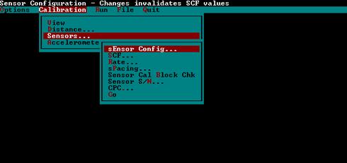
   Figure 30. Screen shot. Sensor calibration menu (2).

2.  
3. Highlight "Sensor Cal Block Chk" and press the Enter key. The monitor will display the calibration check screen shown in figure 31.
   

   
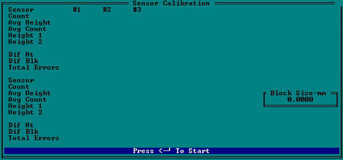
   Figure 31. Screen shot. Calibration check screen (1).

4.  
5. Enter the block size in the window that is open. Type the block size based on the value decided in section "Selection of Calibration Blocks," and press the Enter key to close the window.
6.  
7. Clean the top of the calibration base plates, as needed (base plate is the plate with three feet). Place a calibration base plate on the ground below each sensor, such that the red laser dot is centered on the base plate (see figure 32).
   

   
   Figure 32. Photo. Laser dot centered on base plate (1).

8.  
9. Place a calibration surface plate on top of each calibration base plate, with the long dimension of the calibration surface plate parallel to the long dimension of the profiler sensor bar. Center each calibration surface plate so that the red laser dot of each sensor is centered on the calibration surface plate (see figure 33).

   
   Figure 33. Photo. Calibration surface plate on top of base plate (1).

10.  
11. Press the Enter key to begin sampling by the system. The number of samples taken is displayed at the bottom of the screen. The computer monitor at this stage will look similar to figure 34. (Note: values displayed on monitor for count, Avg Height, Avg Count, Height 1, Height 2, Dif Ht, Dif Blk will be different from values shown in figure 34). Allow the system to take at least 500 samples and then press the Backspace key to stop sampling.
    

    
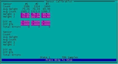
    Figure 34. Screen shot. Readings taken on base plate (1).

12.  
13. Remove the calibration surface plate from calibration base plate for left sensor, then place one of the blocks selected for test on top of the base plate such that the 25 mm side of the block is vertical. Adjust the block so that the red laser dot is at the middle of the block. Place the calibration surface plate on top of the block and adjust the surface plate to ensure the red laser dot is at the middle of the calibration surface plate (see figure 35). Repeat this procedure for the center and right sensors.
    

    
    Figure 35. Photo. Block on top of base plate with calibration plate on top of block (1).

14. Press the Enter key, allow system to take at least 500 readings, and press the Backspace key to stop sampling. The computer monitor at this stage will look similar to figure 36. (Note: Values displayed on monitor for Count, Avg Height, Avg Count, Height 1, Height 2, Dif Ht, Dif Blk will be different from values shown in figure 36).
    

    
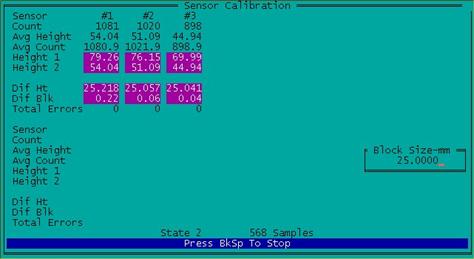
    Figure 36. Screen shot. Readings being taken on 25-mm blocks (1).

    Notations #1, #2 and #3 refer to the left, right, and center sensors, respectively. The value shown in the "Dif Ht" field is the height of block as measured by the data acquisition system in the profiler. The value shown in "Dif Blk" field is the difference between height of block as measured by data acquisition system of the profiler and block height that was entered into the computer in step 3.

15.  
16. Repeat the check for sensor(s) that do not meet specified tolerance if the value displayed in "Dif Blk" for any sensor is outside tolerance of ±0.25 mm. If the value displayed in the field "Dif Blk" for all three positions (#1, #2 and #3) is between +0.25 and -0.25 mm, all three sensors are considered to be functioning satisfactorily. Make sure the system is warmed up, sensor glass is clean, blocks are level, van is steady, and lighting conditions are consistent prior to repeating the test. If the sensor(s) are still outside the tolerance, repeat the test three more times. If tolerance cannot be achieved, turn the engine off, repeat the check, and see if the required tolerance can be achieved. If sensor(s) are still outside the tolerance, move the vehicle to another location and repeat the test. If the operator feels that sunlight may have had an effect on results, move the van to a shaded location and repeat test. If sensor(s) are still outside tolerance, call the RSC to decide on a course of action.
17.  

2.3.3.1.5 Performing Check Individually On a Sensor:

Use the following procedure to perform the laser sensor check on the lasers individually:

1. Select the Calibration option in the MDR main menu, move the highlighted bar to the "Sensors" option, and press the Enter key. The monitor should now display the Sensor Calibration menu shown in figure 30.
2.  
3. Highlight "Sensor Cal Block Chk" and press the Enter key. The monitor will display the calibration check screen shown in figure 31.
4.  
6.  
7. Enter the block size in the window that is open. Type size of block that will be used for the test, and press the Enter key.
8.  
9. Clean the top of the calibration base plate, as needed (base plate is the plate with three feet). Place the calibration base plate on the ground below the sensor that is being checked, such that the red laser dot is centered on the base plate (see figure 32).
10.  
11. Place the calibration surface plate on top of calibration base plate, with the long dimension of the calibration surface plate parallel to long dimension of the profiler sensor bar. Center the calibration surface plate so that the red laser dot is centered on the calibration surface plate (see figure 33).
12.  
13. Press the Enter key to begin sampling by the system. The number of samples taken is displayed at bottom of the screen. The computer monitor at this stage will look similar to figure 37. (Note: Values displayed on the monitor for count, Avg Height, Avg Count, Height 1, Height 2, Dif Ht, Dif Blk will be different from values shown in figure 37). Allow the system to take at least 500 samples and then press the Backspace key to stop sampling.
    

    
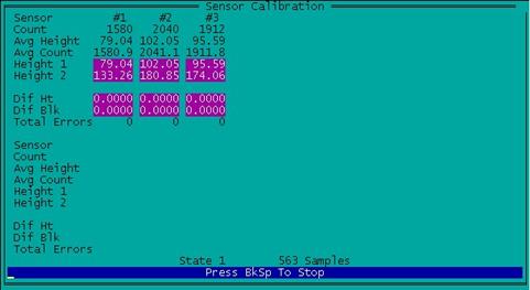
    Figure 37. Screen shot. Reading taken on base plate for single block test.

14.  
15. Remove the calibration surface plate from the calibration base plate, then place the block selected for the test on top of the base plate, such that the 25 mm side of the block is vertical. Adjust the block so the red laser dot is at the middle of block. Place the calibration surface plate on top of the block, and adjust the surface plate to ensure the red laser dot is at the middle of the calibration surface plate (see figure 35).
16.  
17. Press the Enter key, allow the system to take at least 500 readings, and press the Backspace key to stop sampling. The computer monitor at this stage will look similar to figure 38. (Note: The values displayed on the monitor for Count, Avg Height, Avg Count, Height 1, Height 2, Dif Ht, Dif Blk will be different from the values shown in figure 38).
    

    
    Figure 38. Screen shot. Readings being taken on 25-mm block-single block test.

    Notations #1, #2 and #3 refer to the left, right, and center sensors, respectively. The value shown in the "Dif Ht" field is the height of the block as measured by the data acquisition system in the profiler. The value shown in the "Dif Blk" field is the difference between the height of the block as measured by the data acquisition system of the profiler and the block height that was entered into the computer.

18.  
19. Go to step 11 if the value displayed in "Dif Blk" is not within -0.25 mm and +0.25 mm, else go to step 12. If the value displayed in "Dif Blk" for the sensor being checked is between -0.25 mm and +0.25 mm, that sensor is considered to have passed laser sensor check.
    
    Repeat the laser sensor check for the sensor if the value displayed in "Dif Blk" for the sensor is outside the tolerance of ±0.25 mm. Make sure the system is warmed up, the sensor glass is clean, the block is level, the van is steady and the lighting conditions are consistent prior to repeating the test. If the sensor is still outside the tolerance, repeat the test three more times. If tolerance cannot be achieved, turn the engine off, repeat the check, and see if the required tolerance can be achieved. If the tolerance cannot be achieved, move the vehicle to another location and repeat the test. If the operator feels that sunlight may have had an effect on the results, move the van to a shaded location and repeat the test. Once the sensor passes the laser check, go to step 12. If a sensor is still outside tolerance, call the RSC to decide on a course of action.
20.  
21. Repeat steps 3 through 10 for the other two sensors.
22.  

2.3.3.2 Accelerometer Calibration Check

This check should be performed daily prior to data collection to check if calibration values of the accelerometers are within allowable limits. The operator may elect to do a daily accelerometer calibration, following procedures listed in section 2.5.3, instead of a daily accelerometer check.

The accelerometer check should be performed while the vehicle is parked on a level surface. The location where the check is made should be free of any vibrations. Do not bounce or bump the vehicle during this check. The operator may be inside the vehicle with the engine running when this check is performed. The computer should have been turned on and the system warmed up at least 15 minutes prior to performing this check. The following procedure should be used to perform the check:

1. Select "Calibration" to bring up the Calibration menu in the MDR main menu. Next, use the arrow keys to move the highlighted bar to "Accelerometer" and press the Enter key. The Accelerometer Calibration Menu shown in figure 39 will be displayed on the monitor. Make sure the settings shown on the monitor match the values shown in figure 39.
   

   
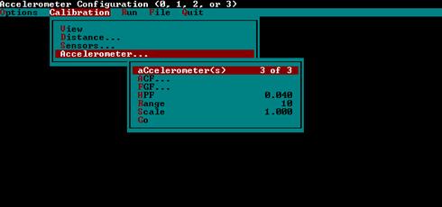
   Figure 39. Screen shot. Accelerometer calibration menu (1).

2.  
3. Use the arrow keys to move the highlighted bar to the "Go" option and press the Enter key. The Accelerometer Calibration screen shown in figure 40 will be displayed on monitor (values shown on the monitor will be different from values shown in figure 40).
   

   
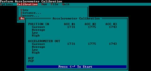
   Figure 40. Screen shot. Accelerometer calibration screen (1).

4.  
5. Press the Enter key and the accelerometer will begin collecting data. After about 5,000 samples have been taken, press the Backspace key to end calibration.
6.  
7. Check the values that are displayed on the monitor for the three accelerometers to see if they are within the allowable range. The allowable range for an accelerometer is normally between 1710 and 1790. However, if during step 25 of the Accelerometer Signal Conditioning Test (see section 2.6.1), the accelerometer calibration factor (ACF) range of an accelerometer was not between 1710 and 1790, a new allowable range for that accelerometer would have been determined as described in section 2.6.2. If any of the displayed values is outside the range from 1710 and 1790, the value must be compared to the range determined according to the procedure described in section 2.6.2 to see if it falls within the allowable range.
8.  
9. Press the "n" key to exit back to the Calibration Menu when the system asks if new values should be accepted. If displayed values are outside the allowable range indicated in step 4, an accelerometer calibration should be performed following the procedures described in section 2.5.3.
10.  

2.3.3.3 Bounce Test

The bounce test is performed to verify that height sensors and accelerometers in the profiler are functioning properly. The bounce test should be performed every day prior to data collection. This test must be performed immediately after the laser sensor check and accelerometer calibration check have been performed. The bounce test consists of two separate tests, a static test and a dynamic bounce test. In the static test, the sensors in the vehicle are turned on while the vehicle is parked, and the generated profile is recorded and evaluated. In the dynamic bounce test, the vehicle is bounced while it is stationary, and generated profile is recorded and evaluated. The vehicle engine may be on or off when performing the static and dynamic bounce tests. Both the static and dynamic tests can be combined into one test. The recommended method for performing the bounce test is the combined test. Procedures for performing the combined test, as well as procedures for performing static and dynamic bounce test separately are described in this section.

2.3.3.3.1 Setup Procedure for Bounce Test:

The following procedures should be followed to setup the profiler prior to performing the bounce test:

1. Park the profiler on a level surface.
2.  
3. Boot up the computer following procedures described in section 2.2.5.4. After the computer has been booted up, WinGraph should be running in system 1, while the monitor should show the MDR main menu (see figure 41). If the computer has already been turned on, use KVM switch and go to system 1. If WinGraph is not running in system 1, double click on the ICC icon to run WinGraph. Then use the KVM switch to go back to system 2.
   

   
   Figure 41. Screen shot. MDR main menu (2).

4.  
5. Turn on the lasers if the lasers have not been turned on.
6.  
7. Select the "Run" option in the MDR main menu and the Run Menu shown in figure 42 will be displayed on monitor.
   

   
   Figure 42. Screen shot. Run menu (2).

8.  
9. Move the highlighted bar to "Options" using arrow keys and press the Enter key. Next, highlight "IRI..." and press the Enter key. The screen shown in figure 43 will be displayed on the monitor. Check to see if Interval is set to 152.4. If not, highlight the Interval, press the Enter key, type 152.4 in the window that opens up, and press the Enter key to close the window. When done, press the Escape key three times to get back to the MDR main menu (figure 41).
   

   
   Figure 43. Screen shot. IRI options screen (2).

10.  
11. Place a brown masonite clipboard below each sensor. This procedure is used because pavement surface texture can affect the IRI values obtained from the bounce test, and placing a clipboard ensures that all three sensors take readings on a smooth and similar surface.
12.  

2.3.3.3.2 Performing Combined Bounce Test:

Power to the computer and lasers should be turned on about 15 minutes prior to conducting the test for electronic equipment to warm up. Use the following procedure to perform combined test, which consists of the static test and dynamic bounce test:

1. Select the "Run" option in the MDR main menu. A Run Menu similar to that shown in figure 42 will be displayed on monitor.
2.  
3. Move the highlighted bar to the "File Name" option and press the Enter key. This will cause a window to open. Type the file name that will be used to save data from the combined test and press the Enter key to close the window. A suggested file name format to follow is YYMMMDDC, where YY-last two digits for current year, MMM - current month (use first three letters of month), DD-current day, and C indicates the test is a combined test.
4.  
5. Select "Options" in the Run Menu (figure 42) and the Run Options screen shown in figure 44 will be displayed on the monitor. Highlight "HW DMI Simulator" and press the Enter key to turn the simulator "On." Press the Escape key once to get to the Run Menu (see figure 42).
   

   
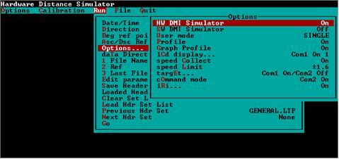
   Figure 44. Screen shot. Run options screen.

6.  
7. Highlight the "Go" option in the Run Menu (see figure 42) and press the Enter key. The monitor should now display a MDR Run screen similar to that shown in figure 45 (values shown on monitor for POS1, POS2, POS3, SEN1, SEN2, SEN3, and filename will be different from that shown in figure 45). The green part of the screen should now display the message OnLineCk. This message indicates that system 2 is connected to WinGraph in system 1. If this message is not displayed, exit the program and go to system 1 and see if WinGraph is running.
   

   
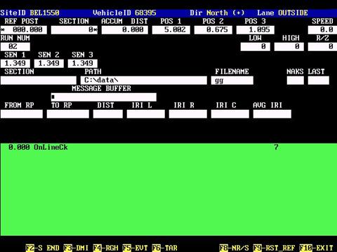
   Figure 45. Screen shot. Run screen of MDR program (1).

8.  
9. Stand outside the vehicle for the static portion of combined test. There should be no motions induced on the vehicle during this test. Press the F3 key to start the DMI simulator. Let the system show a travel of about 600 m, press the F9 key to send a reference reset, and then let the simulator travel for 200 m.
10.  
11. Stand on the rear bumper of the van for the dynamic bounce portion of the test. Bounce the profiler to induce a pitching motion. This motion should pitch the vehicle along the longitudinal direction with no sideways motion. Motion should correspond to a 25 mm displacement of rear bumper for each bounce (i.e., distance from highest position to lowest position is 25 mm during bouncing). For the dynamic bounce test, the IRI value over a distance of 152.4 m within which bouncing motions were induced is evaluated (e.g., this distance may be selected between 304.8 m and 457.2 m, or between 457.2 and 609.6 m). The operator should do some trial runs with another person in order to get an idea about time needed in order to achieve a distance of 152.4 m over which the bouncing motions are performed. Once the operator is sure that bouncing motion was performed between 304.8 and 457.2 m or between 457.2 and 609.6 m, stop bouncing and press the F3 key to stop the DMI.
12.  
13. Go to system 1 using the KVM switch to display the bounce test profile in WinGraph. Move the mouse pointer to the down arrow beside the Y-Scale window on the upper left hand side of the WinGraph window and click on it once with the left mouse button. Move the mouse pointer to the number 1 on the y-scale drop down menu and click it once with the left mouse button (see figure 46). A screen similar to that in figure 47 will be shown at the end of test (IRI values shown on monitor after the test will be different from values shown on figure 47).
    

    
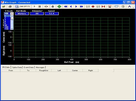
    Figure 46. Screen shot. Adjusting scale of graph in WinGraph.

    
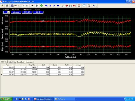
    Figure 47. Screen shot. Output from combined bounce test.

14.  
15. Evaluate profiles that are displayed for the three sensors. The graph should show that the bouncing motion was induced between the limits of 304.8 and 457.2 m or between 457.2 and 609.6 m. If not, the test should be repeated.
16.  
17. Compare profile plots between the three sensors for both the static part and dynamic part of the test. The profile corresponding to dynamic bounce part will show more movement when compared to static portion of the test. Evaluate the profile for the presence of spikes. Spikes in the profile may indicate problems with sensors. Repeat the test if spikes are observed in the profile.
18.  
19. Verify that IRI values from 0 to 152.4 for the left, center, and right sensors are less than or equal to 0.08 m/km. If so, all three sensors are within the tolerance for the static test. If IRI values for the static portion of the test are outside the specified limit, repeat the test. If after repeating the test several times, the IRI value of the sensor(s) is outside the specified limit, decide on a course of action by contacting the RSC. Also, see subsection "Failure of Bounce Test Criterion," which is located after the sections "Performing Static Test" and "Performing Dynamic Bounce Test" in this section.
20.  
21. Select a 152.4 m interval that is shown at the bottom of the graph over which bouncing motions have been performed. This interval may be between 304.8 and 457.2 m or between 457.2 and 609.6 m. Note the IRI value for each sensor for the selected 152.4 m interval, which is IRI of the dynamic bounce part of the test.
22.  
23. Compute the difference between the dynamic bounce IRI and static test IRI for each sensor (left, center, and right). If the difference in IRI is less than or equal to 0.10 m/km for all three sensors, the profiler is considered to have successfully passed the bounce test. If not, repeat the test until all three sensors are within the specified tolerance. If the specified criterion is not satisfied after repeating test several times, decide on a course of action by contacting the RSC. Also, see subsection "Failure of Bounce Test Criterion," which is located after the sections "Performing Static Test" and "Performing Dynamic Bounce Test" in this section.
24.  
25. Obtain a printout of the profile plot if both the static and dynamic IRI criteria are satisfied for all three sensors and note the static test IRI and dynamic bounce test IRI values for each sensor on the graph.
26.  
27. Go to system 2 using the KVM switch. The MDR green color screen will be displayed on the computer monitor.
28.  
29. Press the F10 key to exit program and save data. The system will ask for an End of Run Note. Since none of the given choices are appropriate, press 7 then press the Enter key and type an end of run comment if needed, and press the Enter key.
30.  
31. Press the Enter key if the path and file name to save data that are displayed are acceptable. If a different path and/or file name is needed, use the Backspace key to edit and press the Enter key. After saving the file, the system will revert back to the MDR main menu.
32.  
33. Highlight "Run" in the Main Menu to show the Run menu. In the Run Menu, select "Options" (figure 42) and the Run Options screen shown in figure 44 will be displayed on the monitor. Highlight "HW DMI Simulator" and press the Enter key to turn the simulator "Off." Press the Escape key twice once to get to the Main Menu.
34.  

2.3.3.3.3 Performing Static Test:

The power to the computer and lasers should be turned on for about 15 minutes for electronic equipment to warm up prior to conducting the static test. Use the following procedure to perform the static test:

1. Perform steps 1 through 5 described under the Combined Bounce Test Procedure. In step 3, type an appropriate file name to save the static test data. A suggested file name format to follow is YYMMMDDS, where YY-last two digits for current year, MMM-current month (use first three letters of month), DD-current day, and S to indicates the test is a static test.
2.  
3. Stand outside the vehicle while the static test is being performed. There should be no motions induced on the vehicle during this test. Press the F3 key to start the DMI simulator. Let the system show a travel of about 600 m, press the F9 key to send a reference reset, let the simulator travel for 200 m, and press the F3 key to stop the DMI.
4.  
5. Switch to system 1 using the KVM switch. Move the mouse pointer to the down arrow beside the Y-Scale window on the upper left hand side of the WinGraph window and click on it once with left mouse button. Move the mouse pointer to the number 1 on the y-scale drop-down menu and click once on it with the left mouse button (see figure 46).
6.  
7. Evaluate the profile for the presence of spikes. A screen similar to figure 48 will be shown at the end of the test (IRI values shown on monitor after the test will be different from values shown in figure 48). Spikes in the profile may indicate problems with sensors. Repeat the test if spikes are observed in the profile.
   

   
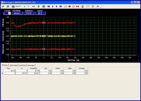
   Figure 48. Screen shot. WinGraph screen after static test has been terminated.

8.  
9. Verify if IRI values from 0 to 152.4 for the left, center, and right sensors are less than or equal to 0.08 m/km. If so, all three sensors are within tolerance. Print the graph and note IRI values from 0 to 152.4 m for the three sensors on the graph. Repeat the test if IRI for any sensor is greater than 0.08 m/km. If after several tests, the IRI value is still outside tolerance, decide on a course of action by contacting the RSC. Also, see section "Failure of Bounce Test Criterion" which follows subsection "Dynamic Bounce Test" in this section.
10.  
11. Switch to system 2 using the KVM switch. The MDR run screen (green colored screen) will be displayed on the computer monitor.
12.  
13. Press the F10 key to exit the program and save data. The system will ask the operator to enter an End of Run Note. Since none of the given choices are appropriate, press 7 then press the Enter key and type an end of run comment if needed, and press the Enter key.
14.  
15. Press the Enter key if the path and file name displayed on monitor are acceptable. If a different path and/or file name is needed, use the Backspace key to edit and press the Enter key. After saving the file, the system will revert back to the MDR main menu.
16.  
17. Turn off the DMI simulator if the Dynamic Bounce test is not being performed after the static test. To turn off the DMI Simulator, highlight "Run" in the Main Menu to show the Run menu. In the Run Menu, select "Options" (figure 42) and the Run Options screen shown in figure 44 will be displayed on the monitor. Highlight "HW DMI Simulator" and press the Enter key to turn the simulator "Off." Press the Escape key twice once to get to the Main Menu.
18.  

2.3.3.3.4 Performing Dynamic Bounce Test:

The dynamic bounce test should be performed after static test has been completed. Use the following procedure to perform the dynamic bounce test:

1. Perform steps 1 through 5 described under the Combined Bounce Test Procedure. In step 3, type an appropriate file name to save data. A suggested file name format to follow is YYMMMDDD, where YY-last two digits for current year, MMM-current month (use first three letters of month), DD-current day, and D indicates test is a dynamic test. The system is now ready to perform dynamic bounce test.
2.  
3. Press the F3 key to start the DMI simulator. Let the simulator travel for about 600 m and then press the F9 key to send a reference reset. Next, stand on the rear bumper of the van and bounce the profiler to induce a pitching motion. This motion should pitch the vehicle along the longitudinal direction with no sideways motion. The motion should correspond to a 25 mm displacement of the rear bumper for each bounce (i.e., distance from highest position to lowest position is 25 mm during bouncing). For the dynamic bounce test, the IRI values between 152.4 m and 304.8 m are evaluated. It will take some time for the operator to get on the bumper and start bouncing after pressing F9 key. Make sure that bouncing motions on the vehicle are induced before a distance of 152.4 m has been reached (the operator should do some trial runs with another person in order to get an idea about time needed in order to achieve this requirement). If bouncing motions started after 152.4, then the bounce test should be continued so that the bouncing motion is induced between distances of 304.8 m and 457.2 m.
4.  
5. Stop bouncing and press the F3 key to stop DMI After a simulated distance of 304.8 m (or 457.2 m if the operator feels that bouncing motions started after 152.4 m). When bouncing the vehicle, the computer monitor cannot be seen. Therefore, estimate the time of bouncing such that the simulator will travel a distance greater than 304.8 m (do some trial runs with another person to estimate time the vehicle should be bounced in order to achieve the specified distance).
6.  
7. Go to system 1 using the KVM switch to display the bounce test profile in WinGraph. Move the mouse pointer to the down arrow beside the Y-Scale window on the upper left hand side of the WinGraph window and click on it once with left mouse button. Move the mouse pointer to the number one on the y-scale drop down menu and click once on it with the left mouse button (see figure 46).
8.  
9. Evaluate the profiles that are displayed for the three sensors. A screen similar to that shown in figure 49 will be shown on the monitor at end of the test (IRI values shown on monitor will be different from values shown in figure 49). The graph should show that the bouncing motion was induced between limits of 152.4 and 304.8 m. If the bouncing motion started after 152.4 m or if the bouncing motion was terminated before 304.8 m, the dynamic bounce test should be repeated. However, if the bouncing motions were continued between the limits of 304.8 to 457.2 m, IRI values within these limits can be used as dynamic bounce test IRI values. In the graph shown in figure 49, bouncing motions started after 152.4 but were continued to a distance greater than 750 m. IRI values between 304.8 and 457.2 m can be used in this case as dynamic bounce test IRI values.

   
   Figure 49. Screen shot. WinGraph screen after dynamic bounce test has been terminated.

10.  
11. Compare profiles between the left, center and right sensors. As there is a time delay after pressing the F9 key and the start of bouncing, the first part of the graph will show the profile recorded during static conditions. A comparison between the static profile and the dynamic bounce profile can also be made by observing the graph. Evaluate the profiles for the presence of spikes. Repeat the test if spikes are noted in the profile. If the bounce test appears to have been performed satisfactorily, note IRI values for the left, center, and right sensors for the distance between 152.4 m and 304.8 m. If bouncing motions commenced after 152.4m and bouncing was performed between 304.8 and 457.2 m, note IRI values between these limits. Print the graph and write down IRI values for the three sensors on the graph.
12.  
13. Compute the difference between the dynamic bounce test IRI and static test IRI for each sensor (left, center, and right). If the difference in IRI is less than or equal to 0.10 m/km for all three sensors, the profiler is considered to have successfully passed the bounce test. If not, repeat the test until all three sensors are within the specified tolerance. If the bounce test criterion is not satisfied after repeating test several times, see the following subsection "Failure of Bounce Test Criterion" in this section.
14.  
15. Go to system 2 using the KVM switch. The MDR green color screen should be shown on the computer monitor.
16.  
17. Press the F10 key to exit the program and save data. The system will ask for an End of Run Note. Since none of the given choices are appropriate, press seven then press the Enter key and type an end of run comment if needed, and press the Enter key.
18.  
19. Press the Enter key if the path and file name to save data are acceptable. If a different path and/or file name is needed, use the Backspace key to edit and then press the Enter key. After saving the file, the system will revert back to the MDR main menu.
20.  
21. Highlight "Run" in the Main Menu to show the Run menu. In the Run Menu, select "Options" (figure 42) and the Run Options screen shown in figure 44 will be displayed on the monitor. Highlight "HW DMI Simulator" and press the Enter key to turn the simulator "Off." Press the Escape key twice once to get to the Main Menu.
22.  

2.3.3.3.5 Failure of Bounce Test Criterion:

If the operator is unable to obtain a static bounce test IRI of less than or equal to 0.08 m/km for a sensor, or if difference in IRI between the dynamic bounce test IRI and the static bounce test IRI exceeds 0.10 m/km, the operator should contact the RSC to decide on a course of action. If an error in the equipment is found and fixed, the operator should reevaluate the profile data that were collected during the previous day. If the problem was in a sensor that is located either in left or the right wheel path, IRI values obtained during the previous day, as well as the profile data, should be compared with those obtained from the last visit to that site. If data problems are suspected, such sections should be reprofiled after equipment repairs.

2.3.4 Data Collection

2.3.4.1 Entering Header Information

Prior to collecting profile data at a site, the operator has to enter header information related to the site. This section describes procedures to be followed to enter header information for a site into the computer, and describes procedures to be followed to get the computer system ready for data collection. Use the following procedures to enter header information at a site:

1. Go to step 2 if the computer has been booted up, otherwise boot up the computer system (using steps outlined in section 2.2.5.3 and 2.2.5.4).
2.  
3. Make sure system 2 is showing the MDR main menu (see figure 50). Use the KVM switch to switch to system 1 and check if WinGraph is running in system 1 (see figure 51). If not, double click on the ICC icon to start WinGraph and use the KVM switch to get back to system 2.

   
   Figure 50. Screen shot. MDR main menu (3).

   
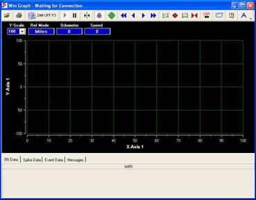
   Figure 51. Screen shot. WinGraph program running in system 1.

4.  
5. Select the Photocell. In the MDR main menu (see figure 50), select Options. The Options Menu shown in figure 52 will be displayed on the monitor. Select "ICC System Parameters" and a screen similar to that shown in figure 53 will be displayed on monitor.

   
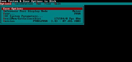
   Figure 52. Screen shot. Options menu (2).

   
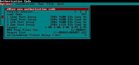
   Figure 53. Screen shot. ICC systems parameters screen.

   The target option in the ICC Systems Parameter Menu (see figure 53) determines which target will send which function key to the data acquisition system when it is tripped. Targets one through three are not used, four is the horizontal photocell, and five is the vertical photocell. F5 refers to an event trigger and F9 refers to the reference reset trigger. Use one of the following procedures to select either the vertical or horizontal photocell to send a reference reset:

   1. Highlight "Target" in the ICC Systems Parameter menu (see figure 53) and press the Enter key. Highlight "Target 5," and use the Enter key to toggle through the available options to select F9. If Target four is showing NA, then press the Escape key twice to get back to the Options Menu (see figure 52). If Target 4 is not showing NA, highlight Target four and use the Enter key to toggle through the available options to select NA, then press the Escape key twice to get back to the Options Menu. Available options when toggling for either Target four or five are NA, F5, F8, F9, and F2. When done, highlight Save Options and press the Enter key to save parameters that were assigned.
   2.  
   3. Highlight "Target" in the ICC Systems Parameter menu (see figure 53) and press the Enter key. Highlight "Target 4," and use the Enter key to toggle through the available options to select F9. If Target five is showing NA, then press the Escape key twice to get back to the Options Menu (see figure 52). If Target 5 is not showing NA, highlight Target 5 and use the Enter key to toggle through available options to select NA, then press the Escape key twice to get back to the Options Menu. Available options when toggling for either Target four or five are NA, F5, F8, F9, and F2. When done, highlight Save Options and press the Enter key to save parameters that were assigned. It has been reported that although the photocell to send a Reference Reset is selected as described above, both photocells still remain active. For example, if Target five (vertical photocell) is set to F9 to send a reference reset with Target four (horizontal photocell) set to NA, the system will still send a reference reset if Target 4 detects a condition that generates an event mark. Therefore, the operator should use a piece of tape to cover the photocell that is not being used. For example, if the operator is specifying the vertical photocell to send a Reference Reset, the horizontal photocell should be covered with a piece of tape.
   4.  
   5. Select the Run option in the MDR main menu. The Run Menu similar to that shown in figure 54 will be displayed on the monitor.

      
      Figure 54. Screen shot. Run menu (3).

   6.  
6.  
7. Highlight "Options" in the Run Menu to bring up the Run Options Menu (see figure 55). In this menu, select IRI and press the Enter key. The IRI options menu shown in figure 56 will be displayed on the monitor. Check if the Interval is set at 152.4. If not, highlight Interval and press the Enter key. When a window opens up, type 152.4 in the window and press the Enter key. Press the Escape key twice to get back to the Run Menu (see figure 54).

   
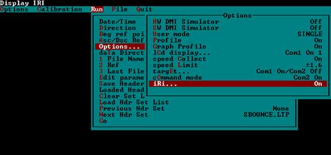
   Figure 55. Screen shot. Run options menu (2).

   
   Figure 56. Screen shot. IRI options screen (3).

8.  
9. Select the Data Directory. In the Run Menu (see figure 54), check to see if the data directory that is shown is appropriate to save profile data. If the directory needs to be changed, highlight "Data Directory" and press the Enter key. This will open a window that shows the current data directory. Use the backspace key to edit the entry shown, type the path (e.g., c:\data\ohio), and press the Enter key to close the window. If the directory that was typed does not exist, the program will automatically create it when it saves the first file.
10.  
11. Retrieve the header file. If a header file for the site does not exist, go to step 8. If a header file has already been created for the site during the previous site visit, load the header file using the following procedure:
    1. Highlight "Load Hdr Set List" in the Run Menu (see figure 54) and press the Enter key. A window will open as shown in figure 57 that shows all the header files that have been created.
    2.  
    3. Highlight the appropriate header file and press the Enter key, then press the Escape key. The selected header file name will be shown under "Next Hdr Set."
    4.  
    5. Select "Edit Parameters - LTPP" and press the Enter key. The LTPP parameters screen similar to that shown in figure 58 will be displayed on the monitor (values for parameters shown on the monitor will be different from the values shown in figure 58).
    6.  
    7. Go to step 9.

       
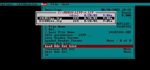
       Figure 57. Screen shot. Header file list.

    8.  
12.  
13. Highlight the "Edit Parameters - LTPP" option in the Run Menu (see figure 54) if a header file is not available for the site, and press the Enter key. The monitor will display a LTPP Parameters screen similar to that shown in figure 58 (values for parameters shown on monitor will be different from the values shown in figure 58).

    
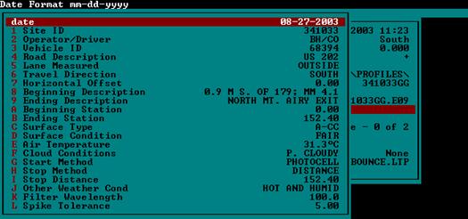
    Figure 58. Screen shot. LTPP parameters screen.

14.  
15. Change selected fields in the LTPP parameter screen to reflect the parameters appropriate for the current data collection if the header file has already been created. The fields that need to be checked for changes are: Operator/Driver, Surface Condition, Air Temperature, Cloud Conditions, and Other Weather Conditions. However, it is a good practice to check all the header fields to make sure they are correct.

    If a header file for the site is not available, all header fields have to be entered/checked to ensure that parameters that are appropriate for the current profile data set are shown in the header.

    The up and down arrow keys can be used to highlight any item in the LTPP Parameter screen that needs to be changed. After the item is highlighted and the Enter key is pressed, a window will open for some items (e.g., Site ID, Operator/Driver). The required value can then be entered in the window and when the Enter key is pressed the window will close. The typed value will be shown for that parameter. Some of the parameters have a specified set of input values, and when these parameters are highlighted, the Enter key can be used to cycle through input options that are available for those items. For example, valid entry for Lane is either Inside or Outside. When Lane is highlighted and the Enter key is pressed, the parameter for lane will cycle between Inside and Outside. The following sections will describe the parameters to be entered or selected for each of the items shown in the LTPP Parameters Menu:

    1. Site ID: Highlight "Site ID" and press the Enter key. Type the site ID in window (e.g., 451024) and press the Enter key to close the window. Follow the procedure described in steps 1 and 2 of section 2.2.7.3 to obtain the appropriate six-digit code for the Site ID. For WIM sites, follow the procedure specified in section 2.4.2.3.
    2.  
    3. Operator/Driver: The operator and driver should be identified by two digit characters, the first letter of their first and last names. Operator and driver names should be separated by a backslash and typed in capital letters (e.g., CK/RS). If the profiler is used as a one person operation, the operator and driver name would be the same (e.g., CK/CK). If the current entry in this field does not correspond to the operator/driver, highlight "Operator/Driver," press the Enter key, type the operator and driver initials in the window, and press Enter key to close window.
    4.  
    5. Vehicle ID: The last five digits of the VIN should be shown in this field. Once this parameter has been set to the correct value, it does not need to be changed. To set the value the first time, highlight "Vehicle ID" and press the Enter key. In the window that opens, type the last five digits of the VIN and press the Enter key to close window.
    6.  
    7. Road Description: Highlight "Road Description" press the Enter key, type the route number where section is located (e.g., I-88), and press the Enter key to close the window. All letters should be capital.
    8.  
    9. Lane Measured: The valid entries for the field are INSIDE or OUTSIDE. The outside lane is the lane adjacent to shoulder at right edge of road. Highlight "Lane Measured," use the Enter key to toggle between INSIDE and OUTSIDE, and select the appropriate value. For nearly all LTPP sections, the lane measured is OUTSIDE.
    10.  
    11. Travel Direction: Select appropriate lane direction (NORTH, EAST, SOUTH, or WEST) by highlighting the field and using the Enter key to bring up the Direction window. Type the first character of direction to add the direction.
    12.  
    13. Horizontal Offset: The value for horizontal offset should be 0 (zero) for all sections. This value has to be set only once, as the system will retain the specified value. Highlight the field, press the Enter key, type 0 in window that opens, and press the Enter key again to close the window.
    14.  
    15. Beginning Description: Enter the milepost at the beginning of the section in this field. If the milepost is not known, enter NONE in this field. An entry in this field can be edited by highlighting "Beginning Description" and pressing the Enter key, which will cause a window to open up containing the current entry in this field. After editing, press the Enter key again to close the window.
    16.  
    17. Ending Description: This field should indicate NONE. An entry in this field can be edited by highlighting "Ending Description" and pressing the Enter key, which will cause a window to open up containing the current entry in this field. After editing, press the Enter key again to close the window.
    18.  
    19. Beginning Station: This field should be set to 0 for all sections. An entry in this field can be edited by highlighting "Beginning Station" and pressing the Enter key, which will cause a window to open up containing current entry in this field. After editing the current value to set the value in field to 0, press the Enter key again to close the window.
    20.  
    21. Ending Station: This field should be set to the length of test section. For GPS and SMP sections, the ending station will always be 152.4. For WIM sections, the ending station should be 305 m. For SPS sections, the ending station will be the total length of the SPS project that is being profiled. An entry in this field can be edited by highlighting "Ending Station" and pressing the Enter key, which will cause a window to open up containing the current entry in this field. After setting the entry in the field to desired value, the Enter key should be pressed again to close the window.
    22.  
    23. Surface Type: Valid entries for road surface type are A-CC for asphalt surfaced pavements and P-CC for PCC surfaced pavements. When "Surface Type" is highlighted, pressing the Enter key will toggle the entry in this field between P-CC and A-CC. Select the appropriate entry.
    24.  
    25. Surface Condition: This describes the surface condition of pavement. Valid entries are V. GOOD (Very Good), GOOD, FAIR, or POOR. When "Surface Condition" is highlighted, the Enter key will toggle between V.GOOD, GOOD, FAIR, and POOR. Select the appropriate entry. Severity levels that are described correspond to the definitions given in the LTPP Distress Identification Manual.⁽¹⁰⁾ The following guidelines should be used to determine road conditions:
        1. V. GOOD: Pavement does not show any distress.
        2.  
        3. GOOD: Pavement exhibits few visible signs of surface deterioration. Asphalt surfaced pavements may show low severity cracks, and Portland Cement Concrete (PCC) pavements may show low severity cracks and spalling.
        4.  
        5. FAIR: Typical distresses on AC surfaced sections can include the following distresses in a low to medium severity: rutting, block or edge cracking, transverse and longitudinal cracking, and patching. Typical distresses on PCC pavements can include the following distresses in a low to medium severity: spalling, transverse and longitudinal cracking, faulting, and patching.
        6.  
        7. POOR: Pavements in this category have deteriorated to such an extent that they affect the speed of free flow traffic. Typical distress on asphalt-surfaced sections includes the following distresses in a medium to high severity: rutting, transverse and longitudinal cracking, alligator cracking, and potholes. Typical distress on PCC pavements can include the following distresses in a medium to high severity: spalling, transverse and longitudinal cracking, faulting and patching.
        8.  
    26.  
    27. Air Temperature: Air temperature (in degrees Centigrade) at time of test should be entered in this field. Obtain air temperature from the temperature display gauge. Highlight "Air Temperature," press the Enter key, enter the air temperature value in the window, and press the Enter key to close the window. If no change to this field is made during subsequent runs, the entered temperature value is saved with profile data for subsequent runs. The operator should note the air temperature prior to the start of each profile run. If the temperature display gauge indicates a temperature that is not within ±2°C of that measured during the previous run, the operator should enter the new value to the software prior to commencing the profile run.
    28.  
    29. Cloud Conditions: Valid entries for this field are CLEAR, P. CLOUDY (Partly Cloudy), or CLOUDY. Use the following guidelines: Clear-sunny sky, Cloudy-sun cannot be observed, P. Cloudy-sun is sometimes covered by clouds. Highlight "Cloud Conditions" and press the Enter key to toggle between CLEAR, P. CLOUDY, and CLOUDY. Select an appropriate entry.
    30.  
    31. Start Method: The start method should always be Photocell. When "Start Method" is highlighted and the Enter key is pressed, entries will toggle between PHOTOCELL and PENDANT. Once this entry is set to PHOTOCELL, it does not need to be changed again.
    32.  
    33. Stop Method: The stop method should always be DISTANCE. When "Stop Method" is highlighted and the Enter key is pressed, entries will toggle between PHOTOCELL, PENDANT, and DISTANCE. Once this entry is set to DISTANCE, it does not need to be changed again.
    34.  
    35. Stop Distance: The stop distance for GPS and SMP sections should be 152.40 m. The Stop Distance for WIM sites should be 305 m. The distance to be entered for SPS sections is presented in section 2.4.1.2. Highlight "Stop Distance," press the Enter key, enter the value in the window, and press the Enter key to close window.
    36.  
    37. Other Weather Conditions: Valid entries for this field are CONDITIONS OK, STEADY CROSSWIND, WIND GUSTS, HOT AND HUMID, HAZY, and LOW SUN ANGLE. Highlight "Other Weather Cond," press the Enter key to toggle through the available entries, and select an appropriate entry.
    38.  
    39. Filter Wavelength: The filter wavelength should be set to 100. Once this value is set, it should not be changed again, as the system will retain this value (value can be changed by highlighting "Filter Wavelength," pressing the Enter key, then typing a value in the window that opens, and again pressing the Enter key to close the window).
    40.  
    41. Spike Tolerance: The required value for spike tolerance is 5.0. To set the value, highlight "Spike Tolerance," press the Enter key, type the value in the window that opens and press the Enter key to close the window.
    42.  
    43. Save Header File: Press the Escape key to get out of the LTPP Parameters screen and to get back to the Run Menu (figure 54). Then highlight "Save Header Params" and press the Enter key. In the window that opens, type the file name to save the header file. The six digit site ID (State code plus the four digit site number) or the file naming convention described in section 2.2.7.3 can be used as the file name to save the header.
    44.  
16.  

2.3.4.2 Profiling Test Section

Once header information has been entered and equipment has warmed up sufficiently (allow 15 minutes after turning power to computers and lasers for equipment to warm up), the profiler is ready to begin profiling. In these procedures, function keys (e.g., F3, F6) have to be pressed. Keys in either the keyboard or the handheld event pad can be used to enter function keys. The following procedures should be followed to get an acceptable set of runs at GPS, SMP, and SPS sites (some of the procedures for profiling WIM sites are different from the procedures presented in this section, see section 2.4.2.3 for procedures for profiling WIM sections):

1. Check if WinGraph is running in system 1. If not, double click on the ICC icon to run WinGraph (if in system 2, use the KVM switch to go to system 1, and use this switch again to get back to system 2 from system 1).
2.  
3. Select "Run" in the MDR main menu to bring up the Run Menu shown in figure 59 (the values shown for the various parameters on the monitor will be different from the values shown in figure 59).

   
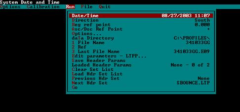
   Figure 59. Screen shot. Run menu (4).

4.  
5. Highlight "Go" in the Run Menu and press the Enter key. The monitor will display the MDR run screen shown in figure 60. The message "OnLineCK" should appear on the green part of the screen. This message indicates the MDR program has successfully linked up with WinGraph (the values shown for POS1, POS2, POS3, SEN1, SEN2, SEN3, and filename on the monitor will be different from the values for these parameters shown in figure 60). The path and filename that are shown will be path and file name that were typed in steps 6 and 7 of section 2.3.4.1.

   
   Figure 60. Screen shot. Run screen of MDR program (2).

6.  
7. Attain a constant test speed of 80 km/h at least 175 m before the beginning of the test section and align the vehicle along the wheel paths (as described in section 2.2.7.4, a speed different from 80 km/h may be used depending on site conditions). Then press the F3 key to start the DMI about 150 m before the start of the test section. (Note: The profiler should have attained its testing speed prior to pressing the F3 key).
8.  
9. Press the F6 key about 40 m before the start of the section (after passing the lead in stripe of the section). When the F6 key is pressed, the asterisk beside the zero in the section field will disappear. When the F6 key is pressed, the photocell is armed and will be looking for the reflective mark on the pavement surface or a cone with reflective marking (depending on photocell that was selected) to record an event mark and perform a reference reset.
10.  
11. Clean the photocell and repeat the run to see if the photocell triggers if vertical photocell is not triggered when event mark is passed. When the photocell detects a target, the green part of screen will show the message "Reference Reset," and a beep will be heard. If the vertical photocell still fails to trigger, adjust the threshold control for the photocell and see if photocell will trigger. If this is not successful, use the horizontal photocell. Follow the procedure described in step 3 of section 2.3.4.1 to select the horizontal photocell to send a Reference Reset.
12.  
13. Press the F3 key to end data collection after the end of the section is passed. (Note: The operator should press the F3 key while the profiler is still traveling at the testing speed.)
14.  
15. Bring the vehicle to a stop at a suitable location to enter an end of run comment, evaluate the collected data, and save the data to hard disk. After stopping the vehicle, use the KVM switch to go to system 1. A graphical output of the profile data collected along the left, center, and right paths will be displayed on the monitor. A vertical line will be present at locations where spikes exceeding the specified spike height (specified in step 30 of section 2.3.4.1) are present. Evaluate profile data for the left, center, and right paths to see if they are satisfactory. IRI for the left, center, and right paths of the section will also be displayed below the graph. Evaluate IRI values and see if they are reasonable. If data appears to be reasonable, go to system 2 using the KVM switch. If the profile data are unreasonable, investigate and correct the problem, and restart data collection.
16.  
17. Press the F10 key to enter the End of Run Note and save the data. When F10 is pressed, the end of run note screen shown in figure 61 will appear on the computer monitor.

    
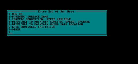
    Figure 61. Screen shot. End of run note screen.

    Evaluate the following six end-of-run comments that are displayed:

    1. RUN OK.
    2.  
    3. PAVEMENT SURFACE DAMP.
    4.  
    5. TRAFFIC CONGESTION: SPEED VARIABLE.
    6.  
    7. DIFFICULT TO MAINTAIN CONSTANT SPEED: UPGRADE.
    8.  
    9. DIFFICULT TO MAINTAIN WHEEL PATH LOCATION.
    10.  
    11. LATE PHOTOCELL INITIATION.
    12.  

    Use guidelines presented in section 2.2.7.8 to select an appropriate end of run comment. The end of run comment should be based on conditions during the profile run, and not based on observations noted in the profile when the profile is evaluated in step 8. If one of the displayed comments is appropriate for the profile run, type the appropriate number and press the Enter key. If none of the displayed comments are appropriate for the profile run and the operator wants to type a different comment, type 7 and press the Enter key. This will open a window where the operator can type an end of run comment. After typing the comment, press the Enter key to close the window.

18.  
19. Save the data. The oath and filename for saving profile data will now be displayed on the monitor. If these are acceptable, press the Enter key. If any changes are needed, use the Backspace key to correct the path and/or file name, and press the Enter key. After the file is saved, the computer screen will show the MDR main menu.
20.  
21. Repeat steps 2 through 10 to obtain five error free runs.
22.  
23. Use ProQual to evaluate the collected data using procedures described in section 2.2.8. As ProQual is a Windows based program, Windows has to be loaded to system 2. Use the following procedure to load Windows to system 2:
    1. Use the KVM switch to go to system 2 if the monitor is showing WinGraph instead of the MDR main menu.
    2.  
    3. Highlight "Quit" in the MDR main menu and press the Enter key.
    4.  
    5. Press "y" to exit system when the MDR Program asks, "Do you want to Exit system?" The C:\ prompt will appear on the monitor.
    6.  
    7. Press the Ctrl - Alt - Delete keys simultaneously to restart the computer.
    8.  
    9. Use the arrow keys to select the Windows option when the Windows 98 menu comes on the screen and press the Enter key.
    10.  
    11. Log in to the system when Windows finishes loading, using LTPP as the user name and LTPP as the password.
    12.  
    13. Start ProQual and evaluate the collected data using procedures described in 2.2.8.
    14.  
24.  
25. Go to step 14 if five runs are acceptable. If not, obtain additional runs as described in section 2.2.8, and review these runs using ProQual.
26.  
27. Use Windows Explorer to backup data to a flash drive or CD ROM. The ICC profile data files that should be backed up are files with file extensions P, V, and E, which were collected at the site. All files generated by ProQual when the profile data were processed (site files) should also be backed up. See section 2.3.5 for a description of ProQual files that should be backed up.
28.  
29. Verify that the LTPP Profiler Field Activity Report Form (see section 2.8.1) and "Status of Regions Test Section" (see section 2.8.2) forms are filled before leaving test site.
30.  

2.3.5 Data Backup

Profile data collected at a site by the profiler and the files generated by ProQual when these data were processed (site files) should be backed up to a flash drive or CD ROM. The computer in the profiler is equipped with a recordable CD drive as well as an Iomega Zip^TM disk drive.

The ICC profile data files that should be backed up are files with file extensions P, V, and E, which were collected at the site.

ProQual data that should be backed up are the site files that were created when the ICC profile data files were processed. The following guidelines for backup of ProQual files are general in nature since there could be variations between directory structures used for ProQual by the different regions. Location of the site files will depend on the directory structure that is employed by the regions to store files generated by ProQual. Figure 62 shows an example of the location of site files that need to be backed up. For this example, data for site 370204 are stored in the directory Sites\37\0204.

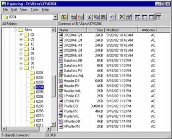
Figure 62. Screen shot. Site files in ProQual.

A recommended procedure to follow during the backup of data for a site is to create separate directories in the backup media (flash drive or CD ROM) for each site.

When a SPS site is processed, separate subdirectories are created for each of the subsectioned sites. The ProQual files created for each of these sections, as well as the raw profile data collected at the SPS site (the P, E, and V ICC files), should be backed up.

The operator should maintain a log to document files that are in each flash drive or CD ROM. The profiler should not leave a test site unless all data have been backed up. At the end of each day, an additional backup copy of all profiler test data collected on that day should be made. Therefore, at the end of each test day, there should be two backup copies that contain profile data that were collected on that day. One of these backups (profiler copy) should be kept in the profiler, while the other copy (RSC copy) should be forwarded to the RSC. Until the RSC copy is forwarded, the profiler copy must be removed from the vehicle whenever testing is not in progress. No collected profile data should be deleted from the hard disk until the RSC has informed the operator that the RSC copy has been received and processed by the RSC. If flash drives are used as a backup medium, the profiler copy of the flash drive can be recycled once the RSC informs the operator that data have been received, processed, and backed up. The RSC should backup the data following procedures outlined in LTPP directive GO-41 "Submission of Electronic Data for Customer Support and AIMS" (or current version of that directive).

WinGraph will save graphical data that are displayed during a profile run, as well as data displayed during the bounce test. These data will be saved in system 1. The path that is specified in system 2 for saving profile data files will be used in system 1 to save the WinGraph data. The WinGraph files do not need to be backed up. They can be deleted after data for the site have been processed by the RSC.

2.4 PROFILING SPS AND WIM SECTIONS

2.4.1 Profiling SPS Sections

2.4.1.1 General Background

This section describes field testing procedures to be followed when testing SPS sites, which are different than the procedures used for GPS sections. However, other than the exceptions described in this section, all other information presented in earlier sections of this manual are valid when SPS sites are being tested. A SPS site consists of a number of test sections with a transition area between adjacent sections. During a profiler run at a SPS site, profile data are collected for entire site, which includes test sections as well as transition areas.

2.4.1.2 Length of Test Sections

Unlike GPS test sections that are always 152.4 m in length, the total length of a SPS project that will include test sections and transition areas will vary from project to project. The operator may elect to break the SPS project into two sections for profiling, depending on the location of the test sections as well as turnaround locations. For example, if there is a large transition distance between two groups of test sections and turnaround is located in the transition area, the operator may elect to profile the SPS project as two sections.

2.4.1.3 Operating Speed

Guidelines regarding operating speed described in section 2.2.7.4 should be followed when testing SPS test sections. When SPS test sections are tested, the transition area between sections may be used to adjust vehicle speed to 80 km/h (or appropriate speed depending on site conditions as described in section 2.2.7.4) before next section is tested. If there is traffic in front of the profiler, the profiler speed can be initially decreased in the transition section to give more leeway between the vehicles in front. Thereafter, the profiler must be brought up to a constant speed of 80 km/h or appropriate speed depending on site conditions before entering next test section.

2.4.1.4 Number of Runs

Five profiler runs in each test section within a SPS project should satisfy the acceptance criteria described in section 2.2.8. ProQual is capable of computing the IRI value of individual test sections within a SPS project by identifying test sections using stationing and event marks. The procedure for subsectioning individual test sections from a profile run made at a SPS section is described in the ProQual manual.⁽⁶⁾ The operator should study IRI computed for each run and plot data from repeat runs to ensure that repeatable data are obtained between runs. The procedure outlined in section 2.2.8 should be followed in order to obtain an acceptable set of runs at a SPS project.

2.4.1.5 Header Generation

The procedures outlined in section 2.3.4.1 for header generation for GPS test sections should also be followed for SPS test sections. However, Stop Distance that is entered in step 27 for a SPS project is different than that entered when profiling GPS sections.

The operator should refer to site layout plans and obtain the length of a SPS project that will encompass all test sections. To guard against discrepancies between layout plans and as built sections, the operator may add a distance such as 30 m to the distance obtained from site layout plan. This distance should be entered as the Stop Distance in step 27 of section 2.3.4.1.

If the operator is not certain about the length to be entered, perform a trial run to determine the length of the SPS project. Go to the MDR run screen (see figure 60) and terminate data collection once the end of the last test section is passed. The MDR Run screen will indicate the location of the Reference Reset and the location where data collection was terminated. Use this information to obtain the length of the SPS project, and enter this length as the Stop Distance.

2.4.1.6 Hardcopy of Profile

The RSC may require the operator to obtain a graphical plot of the data recorded by the left, right, and center sensors for one profiler run of the entire SPS project for archiving and/or quality control purposes. Obtain printouts using data at an appropriate interval such as 400 m. If a printout is obtained, the plot should be attached to the Profiler Field Activity Report. The graphical plot can be obtained using either WinGraph or ProQual. If there are significant differences between profile runs, it is recommended that a graphical plot of profile data be obtained and attached to the Profiler Field Activity Report. In such cases, a plot of all profile runs for each path in one plot or a plot of questionable runs may be obtained.

2.4.1.7 Data Backup

Data collected at SPS projects should be backed up using the same procedures described in section 2.3.5.

2.4.2 Profiling WIM Sections

2.4.2.1 Background

The collection of accurate traffic load (axle weight) data using WIM scales is of vital importance to achieving the LTPP program objectives. Pavement roughness affects the dynamic motion of trucks and therefore the accuracy of traffic load measurements at the WIM scale. Therefore, a smooth pavement section prior to and immediately after the WIM scale is required to minimize those motions.

The pavement smoothness specifications that must be met at WIM sections are not described in this manual. This section describes procedures that should be followed by the RSCs to collect longitudinal profile data at SPS-1, -2, -5, and -6 WIM sections using the LTPP profiler. The resulting profile data will be used to determine if a WIM section meets the LTPP pavement smoothness specifications. (Note: This manual does not contain the procedures to make this determination).

The RSCs are responsible for working with the relevant highway agency to locate and correctly identify the WIM location for each SPS project. Working WIM equipment is not a condition for profiling. SPS projects for which more than one WIM site exist will only be profiled at the site most recently used for data collection. Profiling for SPS projects that are out-of-study will not be done without the explicit direction of the FHWA.

2.4.2.2 WIM Section

A WIM section is defined as a section of pavement that is 305 m long, with the distance from the centerline of the WIM scale to the beginning of the test section being 275 m and the distance from the centerline of the WIM scale to the end of the test section being 30 m.

The WIM section should be marked as shown in figure 63. Monuments (in the form of nails, spikes, or re-bars) should be installed in the shoulders, exactly at the beginning and end of the test section, and at the WIM centerline as shown in figure 63. These monuments will serve as section markers in case of paint wear. The monument at the beginning of the section should be located 275 m prior to the centerline of the WIM scale. The monument at the end of the section should be located 30 m after the centerline of the WIM scale. The distances measured should be accurate to within ±0.10 m. The centerline of the WIM scale is dependent on the sensor used and which of a series of multiple sensors is currently working. For a single sensor installation, the centerline is the middle of the sensor. For a multiple weight sensor array (i.e., bending plates staggered in alternate wheel paths) the centerline is the distance halfway between the approach edges of the first and last weight sensors in the array. Marking the centerline with a monument must avoid all electronics and other elements of the WIM scale installed below the pavement. When the WIM section does not overlap an active LTPP pavement test section, it should be marked by two white stripes, nominally 150 mm wide, across the test lane at the beginning and end of the WIM section. The leave edge of the stripes should be next to the applicable monument. If the WIM section overlaps an active LTPP pavement test section it should not be marked with white stripes.

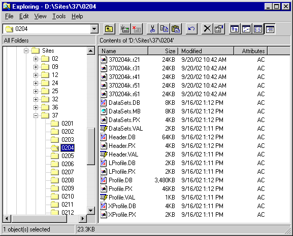
Figure 63. Illustration. Layout of WIM site.

At the centerline of the WIM weight sensor array, one of the following shall be painted near the outside shoulder for permanently marked sites: A WIM SHRP ID of the format PP99, where PP is the Project ID (first two characters of the project SHRP ID) and 99 is the section number assigned for WIM beginning with 99 and decreasing for every new or separate location at which WIM equipment is installed for the project, or the letters WIM.

For example, the Maryland SPS-5 project presently has a piezo system installed in hot-mix AC. The SHRP ID and appropriate marking for this WIM section is 0599. If the piezo system is replaced with the same or a different sensor at another location, the new SHRP ID (and appropriate new marking) for this new WIM section is 0598.

If permanent markings are not in place at the WIM sections, temporary markings such as tape, cones, or other means appropriate to the requirements of the LTPP inertial profilers may be used to trigger the start of data collection. However, the RSCs are responsible for working with the relevant highway agency to ensure that their WIM sections are permanently marked prior to the second visit to the site.

2.4.2.3 Profile Measurements

2.4.2.3.1 General:

Longitudinal profile measurements for smoothness evaluation of LTPP SPS-1, -2, -5, and -6 WIM sections fall into one of the following categories:

1. Verification of existing WIM sections: These WIM sections are already in operation, but they will be evaluated to determine if they satisfy the specified smoothness criteria.
2.  
3. Acceptance of newly constructed WIM sections: Newly constructed WIM sections will be evaluated to determine if they satisfy the specified smoothness criteria.
4.  
5. Annual check of WIM sections: Newly constructed WIM sections that are accepted into the LTPP program, as well as existing WIM sites that have been verified and accepted into the LTPP program, will be monitored once a year to determine if they satisfy the specified smoothness criteria.
6.  

Profile measurements for use in the first two applications will typically be required only once unless special circumstances exist. Furthermore, they will not be done without explicit instructions from the FHWA. Longitudinal and transverse profile measurements using a straightedge will also be made for acceptance testing of newly constructed WIM sections, but applicable data collection procedures are not described in this manual.

With respect to the third category, installed SPS-1, 2, -5, and -6 WIM sections should be profiled during scheduled profile visits to their associated SPS projects. An installed section is a location at which sensors currently exist and at which data has been or is currently being collected. It may or may not be located within the project limits or immediate proximity to the SPS project. Only the LTPP lane will be profiled. In cases where the WIM site is not in the immediate proximity of the project or is in a different direction, the outside lane will be considered equivalent to the LTPP lane.

All profile measurements shall be done exclusively with the LTPP inertial profilers; the Dipstick^® cannot be used as a substitute for the inertial profilers. In addition, the profile measurements shall be performed in accordance with the guidelines and procedures described previously in this manual, except that the procedure for profiling a section and the number of acceptable runs that are required at a WIM section are different from the procedures described in this manual. Procedures for profiling a WIM section and the number of profile runs that are required at a WIM section are described in the next sections.

2.4.2.3.2 Profiling Paths and File Naming Convention:

Profile data collected at three lateral positions are used to evaluate pavement smoothness at WIM sections. The three lateral positions along which the profiler shall be driven to collect the data are the following:

1. Along the wheel paths.
2.  
3. Close to the shoulder (right of the wheel path).
4.  
5. Close to the inner edge of the lane (left of the wheel path).
6.  

The following convention should be followed for naming files. Failure to adhere to this file naming convention could produce errors when running ProQual, and will cause problems when archiving files. The filename should consist of eight characters as follows:

SSDXLPEV

Where:

SS = State code in which the site is located (e.g., 27 for Minnesota).

D = First character of the SPS project SHRP ID, which should be 0, A, B, etc., depending on project code (e.g., 0600, A600, B600, etc.) if profiling in the same direction as the SPS project. If profiling in a different direction from SPS site, this character should indicate the direction traveled (i.e., E, W, N, S).

X = SPS experiment number, which should be the same number as the second digit of the SPS project SHRP ID (e.g., 5 for project A500).

L = Lane identification. Use O for outer, C for center, or I for inner on two or three lane facilities. In the event that there are more than three lanes in the travel direction, use successive numbers starting with 1 as the outer lane.

P = Path followed along the lane which is right, center, or left (i.e., R, C, or L).

E = Letter code defining section type; for WIM sites, this should always be W.

V = Sequential visit identifier that indicates the visit code for the current profile data collection. This identifier indicates the number of times a set of profile runs has been collected at a site since the site was first profiled. Use an appropriate letter for the current profiling with A used for the first visit, B for the second, etc.

For example, the following are valid data filenames:

• 05A6OCWB: Arkansas SPS-6 WIM site profiled in the travel direction of the SPS project in the outer lane along the center path for the second visit.
•  
• 30S1OLWA: Montana SPS-1 WIM site profiled in the southbound direction in the outer lane along the left path for the first visit.
•  
• 29W6ORWC: Missouri SPS-6 project 29A6 profiled in the westbound direction in the outer lane along the right path at the third visit.
•  

2.4.2.3.3 Data Collection Procedure:

Prior to profile data collection at WIM sections, the RSC should either perform or take steps to ensure the following conditions are met:

1. Daily checks should be performed on the equipment (i.e., laser sensor check, accelerometer calibration check, bounce test).
2.  
3. Highway agency procedures relating to safety issues should be strictly followed (i.e., strobe bar and flashing signal bar on, use of turnarounds, etc.).
4.  
5. Operating speed for collecting profile data should be 80 km/h. If maximum constant speed attainable is less than 80 km/h due to either traffic congestion, or safety constraints, then a lower speed depending on prevailing conditions should be selected. If the speed limit at the site is less than 80 km/h, the site should be profiled at the posted speed limit. If traffic traveling at high speeds is encountered at a test site, it is permissible to increase the profiling speed to 88 km/h.
6.  
7. Photocell should always be used to initiate data collection at the beginning of test section.
8.  
9. Section number assigned to the WIM should be entered as the Site ID when entering header information into the software.
10.  
11. "Stop Distance" in software should be specified as 305 m.
12.  

An acceptable set of profile runs is three error free runs in the wheel path and one error free run offset to both the right and the left of the wheel path. On completion of the above steps, the following procedure should be followed to obtain an acceptable set of profile runs at WIM sections:

1. Make sure that the end of the WIM section is passed before terminating profile data collection.
2.  
3. Obtain at least three but no more than five profile runs by driving the profiler along the wheel paths.
4.  
5. Obtain at least one but not more than three profile runs by driving the profiler along a path that is as close as possible to the right edge of the traffic lane (i.e., right tire of vehicle aligned as close as possible to white stripe along the edge of the lane). The driver of the profiler should judge the path to be followed based on the site conditions, such that the path followed does not cause any safety concerns.
6.  
7. Obtain at least one but not more than three profiler runs by driving the profiler along a path that is as close as possible to the left edge of the traffic lane (i.e., left tire of vehicle aligned as close as possible to lane divider along the edge of the lane). The driver of the profiler shall judge the path to be followed based on the site conditions, such that the path followed does not cause any safety concerns.
8.  
9. Review the profile runs that were collected along each path after completing data collection. Evaluate the profiles for equipment related spikes following the procedures described in section 2.2.8.2. If the operator has determined that at least three error free runs along the wheel paths and one error free run along each of the other two paths have been obtained at the site, terminate data collection. If the operator believes that at least three error free runs along the wheel paths and one error free run along each of the other two paths have not been obtained, repeat data collection along appropriate path(s) and evaluate the profile data using the procedures described previously. Up to a maximum of five runs along the wheel paths and three runs along the other two paths should be performed.
10.  
11. Use "Profiling of WIM Sites: Data Summary Sheet" included in appendix C to maintain a log of the runs.
12.  
13. Backup the data prior to leaving the site following procedures described in section 2.3.5.
14.  

2.5 CALIBRATION

2.5.1 General Background

As a minimum, a full calibration check of the laser sensors (see section 2.5.4) must be performed at an interval of 30 days. A full calibration check of the laser sensors must also be performed whenever problems are suspected with the laser sensors, or when a sensor is repaired or replaced.

Accelerometers in the profiler should be calibrated if the accelerometer check (see section 2.3.3.2) indicates ACFs are outside the allowable range or if the bounce test (see section 2.3.3.3) indicates a potential problem with accelerometer(s). The operator may elect to calibrate accelerometers daily prior to performing the bounce test. The accelerometers should be calibrated when repairs are performed on the accelerometer(s) or on computer cards associated with the accelerometer(s). The accelerometers should be calibrated at the time a full calibration check (see section 2.5.4) is performed on the laser sensors.

As a minimum, the DMI should be calibrated (see section 2.5.2) at an interval of 30 days or whenever problems are suspected. The DMI should also be calibrated when tires are replaced, suspension repairs are performed, or when wheels are rotated or aligned. The DMI should be calibrated when repairs are performed on the DMI or to computer cards associated with the DMI.

As a minimum, a calibration check must be performed at an interval of 30 days on the temperature probe.

Power to the electronic equipment should be turned on for about 15 minutes prior to performing any calibration or calibration checks so that the electronic equipment is allowed to warm up and stabilize.

2.5.2 Calibration of DMI

The DMI is calibrated by driving vehicle over a known distance to calculate the Distance Calibration Factor (DCF). The operator enters the actual distance traveled in the calibration menu and the computer calculates the DCF.

An accurately measured section of 300 m should be used to calibrate the DMI. This section should be located on a straight portion of roadway that is reasonably level and has low traffic volume. The speed limit at site should be at least 80 km/h. This section should be in an area where the vehicle can be driven at a constant speed without interruptions. This section should be measured with a standard surveying tape using standard surveying procedures. Reflective tape that will trigger the photocell should be placed on the pavement at the start and end of the section, such that the distance between leave edges of the two reflective tapes is 300 m. The reflective tape should be placed on the lane such that the vertical photocell will traverse over the tape when the profiler traverses the test section.

Prior to driving the vehicle in the morning, the operator should check the tire pressure (cold) to ensure that the tire pressure of the rear tires is at 550 kPa (80 psi), which is the manufacturer's recommended value that is listed on the door and the fuel cover. Adjust the tire pressure if needed to make it 550 kPa (80 psi).

The operator should drive the vehicle for about 6 to 8 km at highway speeds prior to calibration so that the tires can warm up. Based on local weather conditions (e.g., cold weather) the operator may need to increase the distance the vehicle should be driven to warm up the tires. The following procedure should be used to calibrate the DMI:

1. Power up the system and boot up the computer using procedures outlined in section 2.2.5.3 and 2.2.5.4.
2.  
3. Select the photocell. The vertical photocell should be selected following the procedures described in step 3 in section 2.3.4.1.
4.  
5. Adjust the tire pressure. Although the cold tire pressure was set to 550 kPa (80 psi), the tire pressure will increase when the tires are warmed up. Adjust the tire pressure of the rear tires so that the tire pressure is between 551 and 586 kPa (80 and 85 psi). Note the tire pressure.
6.  
7. Bring up the calibration menu. In the MDR main menu, choose "Calibration" to bring up the Calibration Menu shown in figure 64.
8.  
9. Enter the distance and tire pressure. In the Calibration Menu highlight "Distance" and press the Enter key. The screen will display the current DCF and the "Go" option. Highlight "Go" and press the Enter key. The system will then prompt the operator for the Calibration Distance. Enter the length of the calibration section, which should be 300, and press the Enter key. The system will prompt user for tire pressure. Enter the tire pressure of the rear tires in psi and press the Enter key (the tire pressure should be between 80 and 85 psi). The distance calibration screen shown in figure 65 will now be displayed on the monitor.

   
   Figure 64. Screen shot. Calibration menu (2).

   
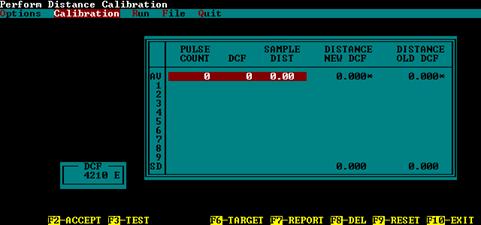
   Figure 65. Screen shot. Distance calibration screen.

10.  
11. Bring the vehicle up to a speed of 80 km/h about 150 m prior to start of the section. Then press the F3 key (to start DMI) followed by the F6 key (to activate the photocell).
12.  
13. Clean the photocell and repeat the run if the photocell fails to trigger. As the profiler crosses the start of the section, a beep will be heard when photocell is triggered by the reflective tape, which is located at the start of the section. When the profiler crosses the reflective stripe at the end of the section, the distance calibration screen will display the new DCF value. If the photocell still fails to trigger, adjust the threshold control for the photocell. If this is not successful, use the horizontal photocell. To use the horizontal photocell, in step 2, select the horizontal photocell as the active photocell. Place two cones on the side of the road at the beginning and the end of the section. Cones placed at the beginning and end of the section should be aligned such that the leave edge of the reflective mark on the cone is aligned with the leave edge of the mark that is on the pavement surface.
14.  
15. Repeat the calibration procedure (steps 6 and 7) five more times so that six calibration runs are obtained. At the start of each run, adjust the tire pressure to the value noted in step 3. If the operator feels that a calibration run was not done properly, move the highlighted bar with the arrow keys to the results and press F8 to delete the run. When six calibration runs have been obtained, the monitor will display a screen similar to that shown in figure 66 (actual values shown on monitor will be different from those shown in  figure 66).

    
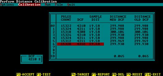
    Figure 66. Screen shot. Calibration screen after obtaining six runs.

16.  
17. Evaluate the Average Distance (as shown in the first line as AV) and standard deviation (as shown at the bottom as SD) under the column "Distance New DCF." If the average distance is within ±0.15 m of actual distance of the site (300 m), and the standard deviation is less than 0.075 m, the DMI calibration has been performed successfully. If the values are outside specified tolerances, obtain additional runs until six runs that meet specified criteria have been obtained. If six runs that meet specified criteria cannot be obtained, contact the RSC to decide on a course of action.
18.  
19. Save the new DCF value that was computed during DMI calibration. Use the arrow keys to highlight the average that is shown at the top and press the F2 key to accept the new DCF value. The system will ask, "Set DCF to Accepted Value?" Press the Y key to save the calibration factor. The program will also save a report for distance calibration. The location of the report (path and file name) will be displayed on the top of the screen when the file is saved.
20.  
21. Press the F10 to exit Distance Calibration. The system will ask "Do You Want to Exit?" Press the Y key to do so, and the MDR main menu will now be displayed on the screen.
22.  
23. Print the Distance Calibration Report that was saved.
24.  

2.5.3 Calibration of Accelerometers

Calibration of the accelerometers should be performed while the vehicle is parked on a level surface. The location where calibration is being performed should be free of any vibrations. Calibration of the accelerometers should not be performed when the engine of the van is running. The operator should be outside of the vehicle when calibration is performed. The operator should adjust the computer monitor so that it can be seen from outside the vehicle and the keyboard should be placed on the seat of the van. Do not enter the vehicle, bounce or bump the vehicle, or lean on the vehicle during calibration. The power to the system should have been turned on for about 15 minutes for the system to warm up prior to calibrating the accelerometers. The following procedure should be used to calibrate accelerometers:

1. Boot up the computer following procedures described in section 2.2.5.4. The MDR main menu should now be displayed on the monitor.
2.  
3. Select "Calibration" in the MDR main menu to display the calibration menu (see figure 67). In the Calibration Menu, highlight "Accelerometer" and press the Enter key, and the Accelerometer Calibration Menu shown in figure 68 will be displayed on the monitor. The settings for parameters displayed on monitor should match values shown in figure 68.

   
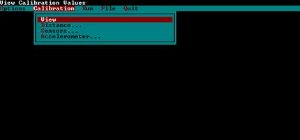
   Figure 67. Screen shot. Calibration menu (3).

   
   Figure 68. Screen shot. Accelerometer calibration menu (2).

4.  
5. Highlight "Go" in the Accelerometer Calibration Menu (see figure 68) and press the Enter key. The monitor will display an Accelerometer Calibration Screen similar to that shown in figure 69 (values displayed on the monitor will be different from those shown in figure 69).

   
   Figure 69. Screen shot. Accelerometer calibration screen (2).

6.  
7. Press the Enter key and the accelerometer will begin collecting data. After about 5,000 samples have been taken, press the Backspace key to end calibration.
8.  
9. Press the N key to repeat the calibration procedure when the system asks if new values should be accepted if test was not valid. If the test appears to be valid, check if all calibration factors are within the allowable range. The allowable range for an ACF is normally between 1710 and 1790. However, if during step 26 of the Accelerometer Signal Conditioning Test (see section 2.6.1), the ACF of an accelerometer was not between 1710 and 1790, a new allowable range for that accelerometer would have been determined as described in section 2.6.2. If any displayed calibration factor is not between 1710 and 1790, check to see if the value is within the range determined according to the procedure described in section 2.6.2. If the calibration factors are within the allowable range, press Y key to accept the values.
10.  

When the Y key is pressed, calibration values are saved and these values will be recorded in the log file. This log file is called cal_log.txt, and it is located in the directory C:\mdrsw\mdr_cal. (Note: The accelerometer calibration screen in the MDR software displays results from accelerometers as positive values. The ACFs are values computed by the software to "zero" the accelerometer reading. The ACFs stored in the MDR software and the calibration log file are negative values.)

2.5.4 Full Calibration Check of Laser Sensors

The laser sensors have been calibrated in the factory and operators cannot calibrate these sensors. A calibration check of the laser sensors is performed prior to data collection (see section 2.3.3.1). In the calibration check, laser sensors are checked to see if they can accurately measure the height within a specified tolerance by using a 25 mm gauge block. However, this procedure only checks the accuracy of the laser sensor over a 25-mm distance within its measuring range. A more comprehensive check of laser sensors should be performed at a minimum interval of 30 days, which will check the accuracy of the laser sensors over a 100-mm measuring range. This check is referred to as the Full Calibration Check of laser sensors to distinguish it from the Calibration Check of laser sensors that is performed prior to data collection in the field. The laser sensor is attached to the sensor bar such that the mid point of the measuring range of the laser sensor is at the ground surface. During a full calibration check, the vehicle is elevated so that the accuracy of the laser sensor over a distance from below the mid point of the measuring range to above the mid point of the measuring range can be checked.

2.5.4.1 Supplies for Calibration Check

2.5.4.1.1 Van Support Blocks:

As described previously, the van is elevated when the full calibration check is performed. This is accomplished by driving the tires of the van over four wooden support blocks, so that all four tires on the van rest on the support blocks. A van support block is made by using two stacked 38-mm by 254-mm by 915-mm boards screwed together on the 254-mm by 915-mm face. One 254-mm end should be beveled to allow the profiler to be driven up onto the blocks. Figure 70 shows an example of a van support block.

Figure 70. Photo. Support blocks.

2.5.4.1.2 Calibration Base Plates:

These are polished steel 100-mm by 100-mm by 9-mm steel plates, with feet installed on the bottom of the plates for stability. Three base plates are provided for each profiler.

2.5.4.1.3 Calibration Surface Plates:

These are polished gray polymer 5-mm by 25-mm by 75-mm plates used as the top reflective surface for the calibration check. Three plates are provided for each profiler.

2.5.4.1.4 Calibration Blocks:

These are polished black polymer blocks having nominal dimensions of 25-mm by 50-mm by 75-mm. Each profiler is provided with six calibration blocks. Each block is engraved with its exact dimension on each face to three decimal places in millimeters.

2.5.4.2 Setup Profiler

Ideally, the full calibration check of laser sensors should be performed in an enclosed building with a level concrete floor, with an external power source (house power) used to power the profiler system. If a full calibration check is performed in the field, the location where the check is performed should protect the profiler from wind and other vibrations. The pavement surface should be as level as possible and lighting conditions should be consistent from sensor to sensor (i.e., face van away from the sun). An external power source should be used, if possible. The following procedures should be used to setup the profiler to perform the full sensor calibration check:

1. Check Sensor Height: The tire pressure can have a significant impact on the sensor height that is obtained. Therefore, the cold tire pressure of all tires must be checked to ensure that they are at the values specified in section 2.2.3.4 prior to performing this check. Make sure power to the laser sensors has been turned off. Remove the sensor covers. With the tires of the profiler resting on floor, measure the distance from the floor to the glass face of the laser sensor. This distance should within ±5 mm of 325 mm. The distance from the ground to the face of the sensor should not change between calibration checks that are performed monthly, unless sensors have been moved or replaced since the previous calibration check. Adjust the sensor if required so that height from the glass face of the sensor to the ground is 325±5 mm.
2.  
3. Clean Sensor Glass: Gently clean each lens with a damp cloth or towel. If excessive dirt is noted on the lenses, wash off loose particles using compressed air or water applied through a sprayer, and then clean the lenses using a damp cloth or towel. When cleaning the lenses, take extreme care to prevent scratching the lenses.
4.  
5. Elevate Vehicle: Place a van support block in front of each tire, and then drive vehicle onto the blocks such that all four tires rest on the van support blocks. Figure 71 shows the van in the elevated position.

   
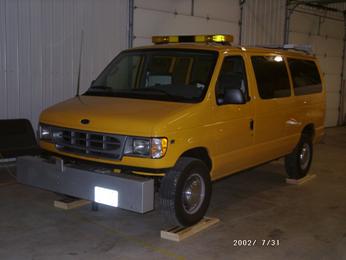
   Figure 71. Photo. Profiler on top of support blocks.

6.  
7. Warm Up Electronics: After connecting to house power, turn on the computer (see sections 2.2.5.3 and 2.2.5.4) and lasers. The monitor should show the MDR main menu. Let equipment warm up for at least 15 minutes.
8.  

2.5.4.3 Performing Full Calibration Check

There are two methods that can be used to perform the full sensor calibration check. In the first method, the calibration check on all three sensors is performed simultaneously. In the second method, the calibration check is performed separately on each sensor. Performing a full sensor calibration check simultaneously on all three sensors will reduce the time required to do this check. Both of these procedures are described in this section.

2.5.4.3.1 All Three Sensors at Same Time:

The following procedures should be used to check all three sensors at the same time:

1. Stand outside the vehicle when the calibration check is performed. Adjust the computer monitor so that it can be seen from outside the vehicle, and place the keyboard on the seat of the van. Do not enter the vehicle, bounce or bump the vehicle, or lean on the vehicle during the calibration check.
2.  
3. Clean the top of the calibration base plates, as needed, and place a calibration base plate on the ground under each laser sensor, so that the red laser dot on each plate is centered within the plates (see figure 72).

   
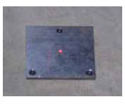
   Figure 72. Photo. Laser dot centered on base plate (2).

4.  
5. Place a calibration surface plate on top of each calibration base plate, with the long dimension of the calibration surface plate parallel to the long dimension of the profiler sensor bar. Center each calibration surface plate so that the red laser dot of each sensor is centered on the calibration surface plate (see figure 73).

   
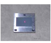
   Figure 73. Photo. Calibration surface plate on top of base plate (2).

6.  
7. Select "Calibration" in the MDR main menu to display the Calibration Menu. In this menu, highlight "Sensors" and press the Enter key to display the Calibration Sensor Menu that is shown in figure 74.

   
   Figure 74. Screen shot. Sensor calibration menu (3).

8.  
9. Highlight "Sensor Cal Block Chk" in the Calibration Sensor Menu and press the Enter key. The monitor will display the sensor calibration screen shown in figure 75.

   
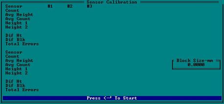
   Figure 75. Screen shot. Calibration check screen (2).

10.  
11. Enter the height of block as 25.0 in the window that opens and press the Enter key (when performing the check with the 50-mm, 75-mm, and 100-mm blocks, enter values of 50.0, 75.0, and 100.0, respectively).
12.  
13. Press the Enter key so that the system will begin sampling (i.e., taking measurements on the calibration surface plates that are below each sensor). The number of samples taken is displayed at the bottom of the screen. The computer monitor at this stage will look similar to the screen shown in figure 76. (Note: Values displayed on the monitor for Count, Avg Height, Avg Count, Height 1, Height 2, Dif Ht, and Dif Blk will be different from those shown in figure 76). Allow the system to take at least 500 samples and then press the Backspace key to stop sampling.

    
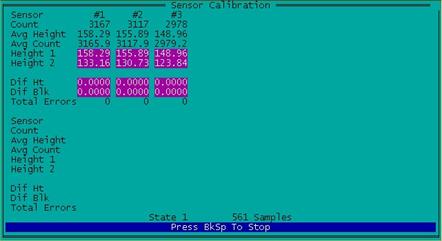
    Figure 76. Screen shot. Readings taken on base plate (2).

14.  
15. Remove the calibration surface plate from the calibration base plate, place the block on top of the calibration base plate such that the 25 mm side of block is vertical, and red laser dot is at the center of the block. Place the calibration surface plate on top of the block and adjust the calibration surface plate such that the red laser dot will be centered on the calibration surface plate. Repeat the procedure for the other two sensors. Figure 77 shows the 25-mm block on the calibration base plate with the calibration surface plate on top of the 25-mm block.

    
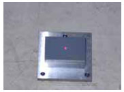
    Figure 77. Photo. Block on top of base plate with calibration plate on top of block (2).

16.  
17. Press the Enter key, allow the system to take at least 500 readings, and press the Backspace key to stop sampling. The computer monitor at this stage will look similar to the screen shown in figure 78. (Note: Values displayed on monitor for Count, Avg Height, Avg Count, Height 1, Height 2, Dif Ht, and Dif Blk will be different from those shown in figure 78).

    
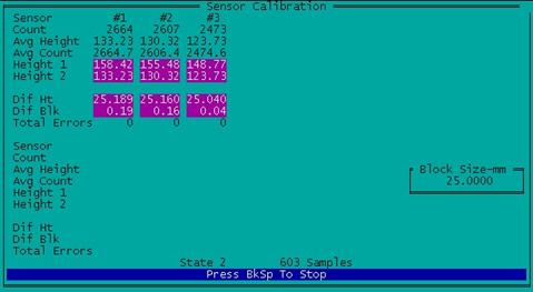
    Figure 78. Screen shot. Readings being taken on 25-mm blocks (2).

18.  
19. Enter the value shown in field "Dif Blk" in the computer to field "Dif Blk From Computer" in form PROF-5 that is included in appendix C (enter for 25-mm block position). Fields #1, #2, and #3 refer to the left, right, and center sensor, respectively. The field "Dif Ht" indicates the height of the block as measured by the data acquisition system in the profiler. The field "Dif Blk" indicates the difference between the height of block as measured by the data acquisition system of the profiler and the block height that was entered into the computer. As the actual heights of the blocks that were placed below the three sensors are not exactly 25 mm, values shown in "Dif Ht" and "Dif Blk" fields have to be adjusted to get correct values.
20.  
21. Enter the height of the blocks that were placed below the left, right, and center sensors in the field "Actual Block Height" in form PROF-5 (values should be entered in columns corresponding to the 25-mm block position with the height of the block entered to three decimal places). Perform computations shown on the form to get values in row numbers three and five.
22.  
23. Repeat the test until the specified tolerance level is achieved for all sensors. If values computed in form PROF-5 for "Adjusted Dif Blk" for all three sensors are between -0.25 mm and +0.25 mm, all three sensors are considered to have passed the full calibration check at the 25-mm position, and the operator should proceed to step 13. If the value for "Adjusted Dif Blk" is outside the specified tolerance of ±0.25 mm, the sensor is out of tolerance. If a sensor is out of tolerance, make sure the system is warmed up, all connections inside the vehicle and outside the vehicle related to the affected sensor are tight, the sensor glass is clean, the blocks are level, the van is steady, and the lighting conditions are consistent. If after five attempts, the sensor(s) is still out of tolerance, contact the RSC and decide on a course of action to resolve the problem.
24.  
25. Repeat steps 6 through 12 for block heights of 50, 75, and 100 mm (in step 6, type in the appropriate block height). For the 50 mm block check, place the blocks under each sensor such that the 50-mm side of the block is vertical. For the 75-mm block check, place the block under each sensor such that the 75-mm side of the block is vertical. For the 100-mm block check, place two 50-mm blocks on top of each other. In step 6, enter block heights as 50, 75, and 100 for the 50-mm, 75-mm, and 100- mm block positions, respectively. When computing "Adjusted Dif Blk" value in form PROF-5, use appropriate columns for each block position. If "Adjusted Dif Blk" at any of these height positions on any sensor is outside the allowable tolerance of ±0.25 mm, resolve the issue following procedures described in the previous step.
26.  

2.5.4.3.2 One Sensor at a Time:

The following procedures should be used to check one sensor at a time:

1. Stand outside the vehicle when the calibration check is performed. Adjust the computer monitor so that it can be seen from outside the vehicle and place the keyboard on the seat of the van. Do not enter the vehicle, bounce or bump the vehicle, or lean on the vehicle during the calibration check.
2.  
3. Clean the top of the calibration base plate, as needed, and place the calibration base plate on the ground under the laser sensor being checked, so that the red laser dot on the plate is centered within the plate (see figure 72).
4.  
5. Place the calibration surface plate on top of the calibration base plate, with the long dimension of the calibration surface plate parallel to the long dimension of the profiler sensor bar. Center the calibration surface plate so that the red laser dot of the sensor is centered on the calibration surface plate (see figure 73).
6.  
7. Select "Calibration" in the MDR main menu to display the Calibration Menu. In this menu, highlight "Sensors" and press the Enter key to display the Calibration Sensor Menu shown in figure 74.
8.  
9. Highlight "Sensor Cal Block Chk" and press the Enter key. The monitor will display the sensor calibration screen shown in figure 75.
10.  
11. Type the dimension of the block to three decimal places in the window that opens. After typing the value, press the Enter key. When starting this test, the shortest dimension of the block that is being used must be entered (the value will be close to 25 mm). The dimension of the block is engraved on the block (when performing the test with other block sizes, the guidelines given in step 13 must be followed).
12.  
13. Press the Enter key to trigger the system to begin sampling (i.e., to obtain measurements on the calibration surface plate). The number of samples taken is displayed at the bottom of the screen. The computer monitor at this stage will look similar to screen shown in figure 79. (Note: Values displayed on the monitor for Count, Avg Height, Avg Count, Height 1, Height 2, Dif Ht, and Dif Blk will be different from those shown in figure 79). Allow the system to take at least 500 samples and then press the Backspace key to stop sampling.

    
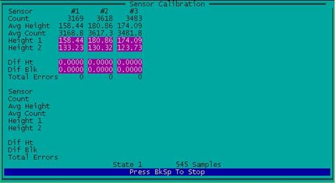
    Figure 79. Screen shot. Readings taken on base plate (base plate below sensor #1).

14.  
15. Remove the calibration surface plate from the calibration base plate, place the block on top of the calibration surface plate such that the 25-mm side of the block is vertical, and the red laser dot is centered on the block. Place the calibration surface plate on top of the block and adjust the calibration surface plate such that the red laser dot will be centered on the calibration surface plate.
16.  
17. 9. Press the Enter key to allow the system to take at least 500 readings, and press the Backspace key to stop sampling. The computer monitor at this stage will look similar to that shown in figure 80. (Note: Values displayed on monitor for Count, Avg Height, Avg Count, Height 1, Height 2, Dif Ht, and Dif Blk will be different from those shown in figure 80).

    
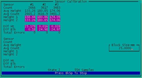
    Figure 80. Screen shot. Readings taken with 25-mm block below sensor #1.

    The field "Dif Ht" indicates the height of the block as measured by the data acquisition system in the profiler. The field "Dif Blk" indicates the difference between the height of the block as measured by the data acquisition system of the profiler and the block height that was entered into the computer. Values displayed for #1, #2, and #3 correspond to left, right, and center sensors, respectively (as the actual block height was entered when doing this test, values for "Dif Ht" and "Dif Block" do not need to be adjusted).

18.  
19. Repeat the test until the specified tolerance level is achieved. If the value displayed in field "Dif Blk" for the sensor being checked is between -0.25 mm and +0.25 mm, the sensor is considered to have passed the full calibration check for the specific block position. If the sensor is within the tolerance, go to step 12. If the value shown in the field "Dif Blk" is outside the specified ±0.25 mm tolerance, make sure the system is warmed up, all connections inside the vehicle and outside the vehicle related to the affected sensor are tight, the sensor glass is clean, the blocks are level, the van is steady, and the lighting conditions are consistent, and repeat the test. If after five attempts the specified tolerance cannot be achieved, contact the RSC and decide on a course of action to resolve the issue.
20.  
21. Record the value displayed in the field "Dif Blk" in the appropriate field of form PROF-6, which is included in appendix C.
22.  
23. Repeat steps 6 through 12 using block heights of 50, 75, and 100 mm for the same sensor, using the following procedure to place blocks and enter values in step 6. For the 50-mm block check, place the block under the sensor such that the 50-mm side of the block is vertical. For the 75-mm block check, place the block under the sensor such that the 75-mm side of the block is vertical. For the 100-mm block check, place two 50-mm blocks on top of each other. At step 6, for each block position, enter the appropriate block height that is engraved on the block (enter the value to three decimal places). For the 100-mm position, add the heights for the two blocks that are being used for the check and enter the value.
24.  
25. Repeat the calibration check for the other two sensors following the procedures described in steps 1 through 13.
26.  

2.5.5 Calibration Check of Temperature Probe

A calibration check on the air temperature probe should be carried out at 30-day intervals. This check can be performed at the time when the full calibration check on the profiler sensors is performed. A temperature probe calibration check log should be maintained in the profiler (form PROF-5 can be used as a log when the laser sensors are checked simultaneously and form PROF-6 can be used when the laser sensors are checked individually). The procedures outlined for the temperature probe calibration check should be followed whenever the operator observes suspicious temperature readings. A National Institute of Standards and Technology (NIST) traceable mercury thermometer is required to perform this test. This test should be performed in the shade, using the following procedure:

1. Park the profiler in the shade and allow some time for the vehicle to cool off if the profiler was exposed to the sun.
2.  
3. Place a thermometer close to the temperature probe and observe the reading of the thermometer.
4.  
5. Record the reading of the temperature displayed by the temperature display gauge in the profiler. If the difference between the two temperature readings are less than or equal to 2 °C, the temperature probe is considered to be acceptable.
6.  
7. Repeat steps 2 through 4 if the difference between the two temperatures is greater than 2 °C. If the difference is still greater than 2 °C, repeat steps 2 through 4 again. If the difference between the temperatures is still greater than 2 °C consider the air temperature probe to be unacceptable and contact the manufacturer of the probe to resolve the problem.
8.  

If there are any questions regarding the accuracy of the temperature probe, a cold temperature check should be performed on the probe. In this check, a plastic bag containing crushed ice is placed around the temperature probe. After allowing a sufficient time for the temperature probe to stabilize, check the reading displayed. The temperature should be within 2 °C of 0 °C.

2.6 EQUIPMENT CHECKS

2.6.1 Accelerometer Signal Conditioning Test

This Accelerometer Signal Conditioning Test checks the power supply, accelerometer filters, and cables to ensure that the analog-digital accelerometer interface card in the profiler is working properly. This test should be performed annually, when problems are encountered with accelerometer readings, or if any repairs have been carried out on the accelerometers or any components associated with the accelerometers. This test is performed using the accelerometer test tool (see figure 81), which consists of a switch with resistors.

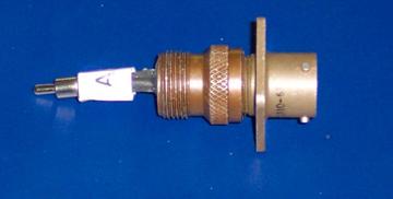
Figure 81. Photo. Accelerometer test tool.

After the accelerometer is unplugged, the test tool is plugged into the accelerometer circuit to perform this test. The following procedure should be followed when performing the test:

1. Park the profiler on a level surface and power up the computer system following the procedures outlined in sections 2.2.5.3 and 2.2.5.4 of this manual. Allow the electronics to warm up for 15 minutes per normal operating procedure.
2.  
3. Calibrate the accelerometers following the procedure described in section 2.5.3 of this manual, and accept the new ACF.
4.  
5. Record the accepted ACF values for the left, right, and center accelerometers in row number 1 on form PROF-8, which is included in appendix C.
6.  
7. Turn off the profiler computer system following the procedures described in section 2.2.5.5.
8.  
9. Unplug the cable from each accelerometer carefully (located under the front bumper near the laser sensors). Attach an accelerometer test tool to each accelerometer cable for the left (driver side), right (passenger side), and center accelerometers, with the switch in position C (or middle position).
10.  
11. Reboot the computer system and launch the MDR program. Ignore the "Invalid Accelerometer Configuration" message and do not recheck the system. Enter Y to operate "with probable error conditions."
12.  
13. Perform an accelerometer calibration following the procedure described in section 2.5.3, but do not accept the ACF values.
14.  
15. Record the ACF values for the left, right, and center accelerometers in row number 2 on form PROF-8.
16.  
17. Move the switch in the accelerometer tool to position A. Perform an accelerometer calibration following the procedure described in section 2.5.3, but do not accept calibration values. ACF values should be negative. If not already indicated on the test tool, mark this position on each accelerometer test tool with permanent ink or with an identification sticker for future tests.
18.  
19. Record the ACF values for the left, right, and center accelerometers in row number three on form PROF-8.
20.  
21. Move the switch in the accelerometer tool to position B. Perform an accelerometer calibration following the procedure described in section 2.5.3, but do not accept calibration values. ACF values should be positive.
22.  
23. Record the ACF values for the left, right, and center accelerometers in row number 4 on form PROF-8.
24.  
25. Move the switch in the accelerometer tool back to position C. Perform an accelerometer calibration following the procedure described in section 2.5.3, but do not accept the calibration values.
26.  
27. Record the ACF values for the left, right, and center accelerometers in row number five on form PROF-8.
28.  
29. Turn off the computer system in the profiler following the procedure described in section 2.2.5.5.
30.  
31. Remove all three accelerometer test tools and reconnect each cable to the accelerometer.
32.  
33. Turn on the profiler computer system using the procedure described in sections 2.2.5.3 and 2.2.5.4 and wait for 10 minutes. Calibrate the accelerometers following the procedure described in section 2.5.3 and accept the new ACF values.
34.  
35. Record the ACF values for the left, right, and center accelerometers in row number six on form PROF-8.
36.  
37. Perform calculations one through five indicated on form PROF-8, and record the values for left, right, and center accelerometers in rows numbered 7 through 11, respectively.
38.  
39. Under Calculation one (row number seven), the computed difference in offset values should be within ±10. If not, this may mean that the internal electronics could be drifting and the RTI-X may need to be replaced. If offset values are not within the range, repeat this test. If accelerometers fail the test again, contact ICC for advice (the accelerometer board may need to be replaced).
40.  
41. The values from Calculations 3 and 4 (rows 9 and 10) should be within ±48. If the resulting values are outside these limits for an accelerometer, a possible problem exists with that accelerometer. Contact ICC to resolve this issue.
42.  
43. The value obtained from Calculation 5 (row number 11), which indicates the difference between post- and pre-test ACF values, should be within ±24 for each accelerometer. If not, there may be too much drift in the accelerometer. Repeat the test, and if an accelerometer fails the test again, ICC should be contacted for further testing/monitoring with the test tool and possible board or accelerometer replacement.
44.  
45. The values obtained when the accelerometer test tool is connected in position A (row number 3) and B (row number 4) should satisfy the following ICC provided criteria: (a) ACF values for Position A should be between -2552 and -2088 (±10 percent of -2320), and (b) ACF values for Position B should be between 1908 and 2332 (±10 percent of 2120).
46.  
47. If any accelerometer fails to satisfy the previously described two criteria, additional observations or testing should be done as follows: (a) If the reason for the failure cannot be determined, contact ICC, (b) If one channel fails while the others pass, examine the wiring for that accelerometer to determine if an open power wire is creating a problem, (c) If all channels are failing, examine all wiring to ensure that a short circuit between the connector pins is not causing the failure. These types of failures generally will change the numbers over 25 percent. If the numbers are less than 25 percent different, but greater than 10 percent, the power supply could be drifting, which indicates an RTI-X problem. Determine the drift using the following procedure: (a) reinstall the test tools (if already removed) following the procedures described previously and (b) repeat the tests for positions A and B two times at two minute intervals to determine the drift. Once drift has been determined, contact ICC to determine if additional testing is required or if any parts need to be replaced.
48.  
49. After the first test is performed with the accelerometer test tool, each subsequent test result for offset 1 and offset 2 should be compared with the prior test value. The test values should be within ±32 (ICC's current estimate). Contact ICC if the difference is outside the allowable range.
50.  
51. Check the ACFs using the procedure described in section 2.3.3.2. If the calibration factor of an accelerometer is not between 1710 and 1790, compute a new allowable range for the ACF following the procedure outlined in section 2.6.2.
52.  

2.6.2 ACF Range

The calibration factor of all accelerometers must be checked to ensure that they fall within the allowable range during the daily accelerometer check (see section 2.3.3.2) and after calibrating the accelerometers (see section 2.5.3). The allowable range of the ACF that was specified by ICC when LTPP took delivery of the profilers was between 1710 and 1790. However, at that time, the ACFs of all accelerometers were not close to the mid-point of the allowable range (i.e., 1750). Some accelerometers had calibration factors that were between the lower bound of 1710 and the mid-range value of 1750. Over time, the ACFs in some accelerometers have been drifting towards the lower bound of the allowable range and may fall below the allowable value of 1710. If the ACF of an accelerometer falls below the lower limit of 1710 or exceeds the upper limit of 1790, the following procedure should be followed to determine a new allowable ACF range:

1. Perform the Accelerometer Signal Conditioning Test described in section 2.6.1. If one or more accelerometers fail the criteria established for that test, follow the recommended procedures to address and resolve the issue.
2.  
3. Go through the records and obtain the calibration factors for the first 10 times the accelerometer was calibrated. If the accelerometer has not been replaced, the values will correspond to the 10 calibration values after the region started to operate the ICC profiler. If an accelerometer has been replaced, the values will correspond to the 10 calibration values after the new accelerometer was installed.
4.  
5. Average the 10 calibration values to obtain an average initial calibration factor value for the accelerometer.
6.  
7. Compute the allowable ACF range for the accelerometer as the average initial calibration factor value (from step 3 above) ± 40.
8.  
9. Use the ACF range computed in step 4 when performing the daily accelerometer check (see section 2.3.3.2) and checking the range of the ACFs after calibrating the accelerometers (see section 2.5.3).
10.  

2.6.3 Photocell Offset Determination

2.6.3.1 Overview

The K. J. Law T-6600 profilers that were used in the LTPP program to collect profile data from 1996 to August 2002 obtained the first data point at a distance of 114 mm from the leave edge of the section start stripe. When the data collected by the ICC profilers are processed by ProQual, in order to be consistent with the data collection procedure used by the K. J. Law T-6600 profilers, the first data point in the test section is assigned a location that is 114 mm from the leave edge of the section start stripe.

ProQual needs a parameter called the photocell offset in order to process that profile data such that the first data point is at the previously indicated location. Separate photocell offsets are needed for the vertical photocell and the horizontal photocell. When ProQual processes profile data, the program uses the vertical photocell offset for cases where data collection was initiated with the vertical photocell, and the horizontal photocell offset for cases where the data collection was initiated with the horizontal photocell.

Each RSC should annually determine the vertical and horizontal photocell offset values using the procedure that is described in sections 2.6.3.2 to 2.6.3.4 and the values must be entered into the ProQual equipment table. The equipment table in ProQual is accessed through the System menu in ProQual (see figure 82). The ProQual copy in the profiler, as well as all ProQual copies in the RSC office that are used to process profile data, should be updated with the photocell offset values that are determined annually.

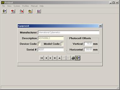
Figure 82. Screen shot. Equipment table in ProQual.

Each RSC should maintain a log that indicates the following related to photocell offsets: date when testing was performed to determine photocell offsets, values obtained for vertical and horizontal photocell offsets, and date when photocell offset values were updated in ProQual.

The following sections describe the field procedure for performing the test and the procedure to perform the computations using the collected data.

2.6.3.2 Site Preparation

The test procedure involves attaching an artificial bump target to the pavement and then collecting a series of profiles with the center laser sensor passing over the bump. The testing location should be a straight stretch of road with very low traffic volume where it is possible to safely attain a profile speed of 80 km/h. As operator safety is of utmost concern, the site location should not place the operator in harm of traffic while attaching the target to the pavement, nor should the traffic at the location present the possibility of disturbing the target while the testing is being performed. The ideal location should be a new or a recently overlaid pavement surface with no significant pavement distresses within 15 m of the target point. Pavements with rough surface textures, such as chip seals or severe raveling, should be avoided.

Once a location for testing has been selected, it is necessary to establish a beginning section mark. Place a 52 to 102 mm wide strip of white or silver adhesive tape at the testing location on the pavement, such that it is perpendicular to the direction of travel and in a location that will be detected by the vertical photocell when the profiler is driven over the location. Select a suitable bump target from a length of wood with the dimensions 13 mm thick, 38 mm wide, and 750 mm long. Place the bump target on the pavement parallel to the previously established starting stripe in a manner such that the 13 mm dimension is vertical to the pavement, the approach edge of the 38 mm dimension is 114 mm from the leave edge of the starting stripe, and the target spans the path that will be traversed by the center laser sensor (approximately mid-lane). The bump target should be positioned in such a way that the right or left tires will not run over it during profile runs. Affix the bump target to the pavement with an appropriate adhesive tape such that the adhesive tape will not affect the profile collected by the center laser. Figure 83 illustrates the positioning of the section stripe and bump target.

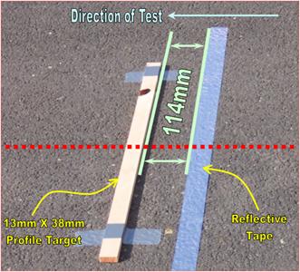
Figure 83. Photo. Section starting stripe and bump target placed on the pavement.

Thereafter, the horizontal photocell target has to be established in relation to the starting stripe. Place the horizontal photocell target on the shoulder of the road in a position that will minimize the potential for disruption during testing. Align the horizontal photocell target such that the leave edge of the reflector is in line with the leave edge of the stripe placed on the pavement. The placement of the vertical and horizontal photocell targets is intended to replicate standard profile operations. Figure 84 illustrates the proper placement of the horizontal photocell target in relation to the starting stripe and bump target.

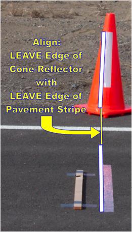
Figure 84. Photo. Placement of vertical photocell target in relation to section starting location.

2.6.3.3 Profile Data Collection

The photocell offset determination is performed in a manner consistent with standard LTPP profile data collection procedures. It is important that the DMI has been calibrated beforehand in accordance with section 2.5.2 of this manual, and the tires in the profiler are sufficiently warmed up with air pressures matching the pressure noted during the DMI calibration. Ideally, the full range calibration check of the profiler's laser sensors should have been performed, in accordance with section 2.5.4 of this manual prior to performing this testing. However, if the full calibration check has not been performed within two days of this testing, perform the standard daily height sensor check and bounce test in accordance with section 2.3.3 of this manual. For this testing, both photocells will be active simultaneously, but two sets of profiles (five runs each set) will be collected for computing offsets for each photocell. For this testing, the profile data of concern is primarily in the region of the bump target. Therefore, it is not necessary to collect a large amount of profile data during each run. Only 40 to 50 m of profile data before and 20 m of profile data after the section start stripe need to be collected. Although processing of the profiles collected during this testing will be described in the next section, verification of the suitability of the profiles should be performed by reviewing the profiles in the ICC WinGraph software and by examining the occurrences of events in the MDR data collection software.

The following procedure should be followed for collecting data:

1. Select the "ICC System Parameters..." option from the "Options" menu of the ICC MDR data collection software to set the desired photocell parameters. In the "Target..." option, set the photocell parameters as follows:
   1. For the horizontal photocell offset runs, set Target 4 = F9 and Target 5 = F5 as shown in figure 85.
   2.  
   3. For the vertical photocell offset runs, set Target 4 = F5 and Target 5 = F9 as shown in figure 86.

      
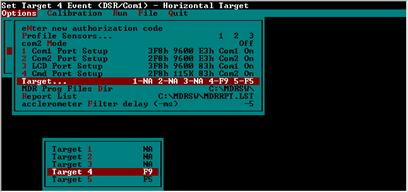
      Figure 85. Screen shot. Photocell target parameters for determining horizontal photocell offset.

      
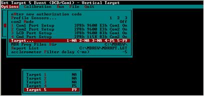
      Figure 86. Screen shot. Photocell target parameters for determining vertical photocell offset.

   4.  
2.  
3. Specify an appropriate data directory from the "Run" menu of the MDR software where the profile data can be stored for easy access and backup.
4.  
5. Specify an appropriate file name from the "Run" menu of the MDR software for the profiles to be collected. Although the format of the file name is not critical for the purpose of this testing, it is necessary that the file name be logical so that the analysis described in next section can be completed. It is recommended that the file naming format from section 2.2.7.3 of this manual be used, with the visit identifier indicating which photocell is being tested.
6.  
7. Set any relevant parameters in the "Edit parameters - LTPP..." option from the "Run" menu of the MDR software.
8.  
9. Make five profile runs over the artificial bump target using the following procedure:
   1. Attain a speed of 80 km/h at least 300 m before the bump target.
   2.  
   3. Select the "Go" option from the "Run" menu of the MDR software to enter the Run screen well in advance of the target.
   4.  
   5. Press the F3 key at least 40 m prior to the start stripe to start the DMI and the F6 key to arm the photocells.
   6.  
   7. Profile over the bump target, and once the profiler is 20 m past the target, press the F3 key to stop data collection.
   8.  
   9. Review the Reference Reset and other events in the run screen for logic and to assure that the assigned photocell in step 1 performed the reference reset.
   10.  
   11. Press the F10 key to exit the run screen and save the data files to the hard disk drive.
   12.  
   13. Repeat steps a through f until five acceptable runs for the assigned photocell have been collected.
   14.  
10.  
11. Repeat steps 1 through 5 for the other photocell.
12.  

2.6.3.4 Photocell Offset calculations

The profile data should be analyzed using the ICC Road Profiler Reporting Program, Winrp90l.EXE (WinReport) Version 1.09, which is stored in system 2. WinReport is a Windows^TM based program and requires that system 2 be booted in Windows 98 in order to run it. The program is capable of using configuration files to store frequently used report parameters, but this procedure does not require that a configuration file be used. The following steps describe the procedures for determining the horizontal and vertical photocell offset values:

1. 1.      Launch WinReport by navigating to the C:\mdrsw\directory and opening the Winrp90l.EXE program. WinReport launches a window that is similar to that shown in figure 87.

   
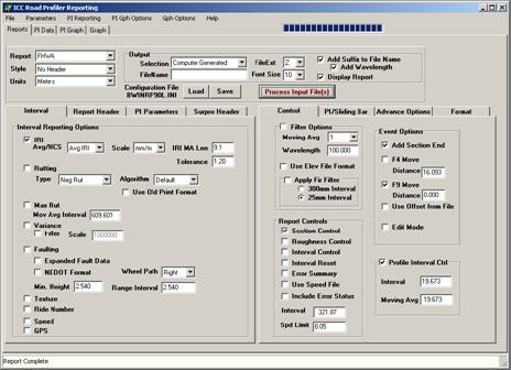
   Figure 87. Screen shot. WinReport program menus.

2.  
3. Select the following parameters in WinReport on the Reports, Interval, and Control tabs as shown in figure 87 (the Reports tab is the primary tab on this window, and the Interval and Control tabs are the left and right secondary tabs, respectively). Select the following parameters:
   1. Select FHWA from the Report dropdown list.
   2.  
   3. Select No Header from the Style dropdown list.
   4.  
   5. Select Meters from the Units dropdown list.
   6.  
   7. Select Computer Generated from the Selection dropdown down list.
   8.  
   9. Select Z from the FileExt dropdown list.
   10.  
   11. Check the Display Report Box.
   12.  
   13. Verify that Font Size is 10, the Add Suffix to File Name box is checked, and the Add Wavelength box is checked.
   14.  
   15. Verify that only the IRI box is checked on the Interval tab. Items on the Interval tab will not influence the outcome of this analysis and the IRI box is checked because some versions of this software require at least one box on this tab be checked, while some versions may work with no boxes checked. Parameters in the Report Header, PI Parameters, and Surpro Header tabs are not used for this analysis.
   16.  
   17. Verify that the Filter Options check box is not selected on the Control tab.
   18.  
   19. Verify that the Section Control box is checked on the Control tab and that no other items in the Report Controls section are checked. The values in the fields Interval and Spd Limit are not used in this analysis.
   20.  
   21. Verify that the Add Section End and F9 Move boxes are selected on the Control tab in the Event Options section. The F9 Move Distance should be 0.0. Verify that the F4 Move, Use Offset from File, and Edit Mode are not selected. The value in F4 Move Distance has no impact on the data analysis.
   22.  
   23. Verify that the Profile Interval Ctrl section is checked and that the Interval and Moving Avg are set to 19.673.
   24.  
4.  
5. Go to the "Advanced Options" tab as shown in figure 88 and select the following parameters:
   1. Verify that the Height Data Only box is checked.
   2.  
   3. Check the From/To Section box and set the first value to -1 and the second value to five.
   4.  
   5. Verify that the Max Delta Profile value is 0.07620.
   6.  
   7. Verify that all other boxes are not checked and that the Position SF value is left blank.
   8.  

   
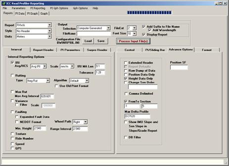
   Figure 88. Screen shot. Parameters set in the advanced options tab.

6.  
7. Select the "Process Input File(s)" button. A file selection window similar to that shown in figure 89 will appear.

   
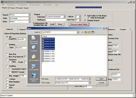
   Figure 89. Screen shot. File selection window in WinReport program.

8.  
9. Highlight the five profile data files that were collected for the horizontal photocell offset determination and select the "Open" button. The software will perform the analysis on each data file individually. At the conclusion of the data analysis, WinReport will open WordPad windows to display the profile data in text format for the five runs, similar to as shown in figure 90.

   
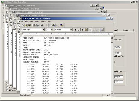
   Figure 90. Screen shot. Text format profile data displayed in WordPad window.

10.  
11. Scroll down through the profile elevations in each WordPad window until the reference reset (REF_RST) event mark is visible as shown in figure 91.
12.  
13. Scan the center profile elevations (third column from left in text file) for the point after the reference reset where the 13 mm bump is apparent in comparison to the remainder of the profile elevations (as highlighted in figure 91).
14.  
15. Record the distance (first column from left in text file) for the first profile elevation that shows the elevation change for the bump target for each of the five profile runs. (Note: The REF_RST may appear on a line that precedes the actual 0.0 m distance. For the purposes of this analysis, all distance measurements are referenced from the zero distance point indicated in the file). In figure 91 this value is 0.256 m.

    
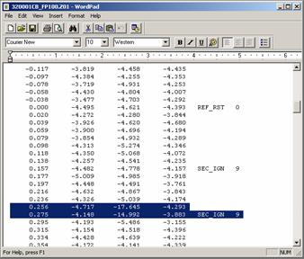
    Figure 91. Screen shot. Profile data displayed in WordPad window-horizontal photocell test.

16.  
17. Average the five values if all five distance values are within 20 mm of each other. If one of the values differs by more than 20 mm from the other four values, discard that value and average the remaining four values. If more than one value differs by more than 20 mm from the remaining values, discard the data, assess the condition of the bump target and photocell target positioning, and perform the testing again as described in section 2.6.3.4.
18.  
19. Repeat steps 4 through 10 for the set of profiles collected for vertical photocell offset determination. The files displayed in the WordPad window for this photocell will be similar to that shown in figure 92.
20.  

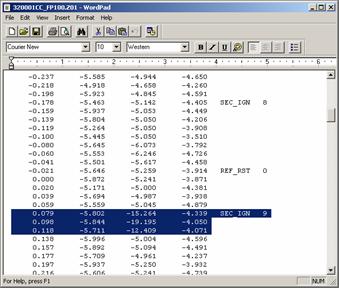
Figure 92. Screen shot. Profile data displayed in WordPad window-vertical photocell test.

The results from step 10 provide the photocell offsets for each photocell. The target bump was placed on the pavement 114 mm upstream of the section starting stripe and the offset values obtained from this experiment reflect the distance at which the first profile elevation value falls on the bump (within an acceptable range). The computed offset values when rounded to the nearest 25 mm are the vertical and the horizontal photocell offsets.

2.7 EQUIPMENT MAINTENANCE AND REPAIR

2.7.1 General Background

Responsibility for equipment maintenance and repair rests with each RSC. Decisions required for proper maintenance and repair should be based on the testing schedule and expedited as necessary to prevent disruption of testing. Maintenance activities on the profiler should be performed prior to mobilization for testing. During a testing period, there will be little time to do more than the required daily checks prior to testing. Specific detailed maintenance procedures are contained in the manuals provided with each piece of equipment (see References). The operator must become familiar with the maintenance recommendations contained in all equipment manuals. Maintenance or repair work to be performed can be classified as routine maintenance, preventive maintenance, and unscheduled maintenance.

2.7.2 Routine Maintenance

Routine maintenance includes work that can be performed by the operator. The Daily Check List (see appendix C) includes a list of maintenance activities to be performed every day. These procedures include checking the vehicle lights, checking under the vehicle for fluid leaks, checking fluid levels in the vehicle, and cleaning the glass covers of the sensors and photocell. These items are the most basic and easily performed maintenance measures and should always be done prior to using equipment every day. If any problems are noted, they should be entered in the Profiler Log (section 2.8.4), which should be maintained in the vehicle, and appropriate action should be taken to correct the noted problems.

Laser height sensors are sealed units and they will not function correctly if the seals are broken. Cracked or chipped glass in the lasers may cause moisture damage to occur and this can lead to failure of the sensor. If any sign of physical damage is noted on the sensor glass, ICC should be contacted to decide on a repair procedure.

2.7.3 Scheduled Major Preventive Maintenance

Scheduled major preventive maintenance services are those that are performed at scheduled intervals. Scheduled preventive maintenance activities on the vehicle should be performed following the manufacturer's heavy use guidelines. These include activities such as oil changes. Drive belts, hoses, battery cable connections, etc., should be checked when the oil is changed in the vehicle.

The LTPP Major Maintenance/Repair Form (see appendix C) should be used by the operator to report the necessary services performed and also serves to inform the RSC of the condition of the profiler on a regular basis.

2.7.4 Unscheduled Maintenance

These are unscheduled repairs. These repairs must be reported on the LTPP Major Maintenance/Repair form as an unscheduled maintenance activity. The LTPP Major Maintenance/Repair form should be completed whenever a sensor is replaced or repaired. The procedures described in section 2.2.3.5 should be followed after a sensor is replaced or repaired.

2.8 RECORD KEEPING

There are eight types of records that should be forwarded to the RSC by the operator. They are

1. LTPP Profiler Field Activity Report.
2.  
3. Status of the Regions Test Sections.
4.  
5. Profiler Log.
6.  
7. LTPP Major Maintenance/Repair Form.
8.  
9. Profiler Calibration and Calibration Check Reports.
10.  
11. Profiling of WIM Sites: Data Summary Sheet.
12.  
13. Accelerometer Signal Conditioning Test Form.
14.  
15. ProQual Reports and Profile Plots.
16.  

A description of each of these forms/reports is presented in the following sections. If items described for the Profiler Log or the LTPP Major Maintenance/Repair form are recorded by the operator following standard operating procedures of the RSC, the completion of these forms may be omitted. It is acceptable for a region to use forms that have a different format as long as the modified form contains all of the items indicated in the forms included in this manual.

2.8.1 LTPP Profiler Field Activity Report

The Field Activity Report (form PROF-1 in appendix C) records all activities to and from a site, as well as activities at the test site. This report should be filled out for all travel and testing days. For travel only days, the section for which traveling is being done should be noted. Entering IRI readings requested on this form is optional. However, the IRI values should be entered if a region keeps this form in the vehicle and uses IRI values as a check when the section is profiled subsequently.

2.8.2 Status of the Regions Test Sections

The Status of the Regions Test Sections form (form PROF-2 in appendix C) should be filled out at every test section. Recent maintenance or rehabilitation activities, condition of paint marks, missing LTPP signs and delineators, as well as any other comments regarding the test section should be recorded on this form.

2.8.3 Profiler Log

The operator should maintain a Profiler Log in the vehicle. The format of the log is shown in form PROF-3 in appendix C. When the operator performs daily checks on equipment, items that need attention should be noted on the Profiler Log.

2.8.4 LTPP Major Maintenance/Repair Form

The LTPP Major Maintenance/Repair form (see form PROF-4 in appendix C) should be completed when scheduled or unscheduled maintenance or repairs are performed on the profiler. Vehicle and equipment operating costs are monitored with this form. This form should be submitted along with all receipts for maintenance activities.

2.8.5 Profiler Calibration Reports

Each time a full calibration check is performed on the laser sensors, either form PROF-5 (if all sensors are checked simultaneously) or PROF-6 (if sensors are checked individually) should be completed. Both forms are included in appendix C. The appropriate form (PROF-5 or PROF-6) should also be used to record information related to DMI calibration, accelerometer calibration, and the calibration check on the temperature gauge. After a calibration is performed on the DMI, a printout of the calibration report should be obtained and attached to the calibration form (PROF-5 or PROF-6). The Profiler Calibration Reports should be maintained in a three ring binder.

The operator should regularly backup the calibration log file, as past accelerometer calibration values are stored in this file. The log file is called cal_log.txt, and it is located in the directory C:\mdrsw\mdr_cal.

2.8.6 Profiling of WIM Sites: Data Summary Sheet

The operator is required to complete the Profiling of WIM Sites: Data Summary Sheet (see form PROF-7 in appendix C) when profile data are collected at a WIM site.

2.8.7 Accelerometer Signal Conditioning Test

The form PROF-8 in appendix C should be completed when performing the Accelerometer Signal Conditioning Test.

2.8.8 ProQual Reports and Profile Plots

The Site Visit Report generated by ProQual contains a statistical summary of IRIs for different runs at a test site. The Site Visit Report must be attached to the associated Field Activity Report. If a graphical output of profile data is obtained at a site, the printout should be attached to the associated Field Activity Report. RSCs may elect to print the Site Summary Report generated by ProQual in addition to the Site Visit Report. If the Site Summary Report is printed, it must also be attached to the Field Activity Report. RSCs may also elect to print the Spike Report generated by ProQual and attach it to the Field Activity Report.

 

<< Previous

Contents

Next >>