Long-Term Pavement Performance Computed Parameter: Frost Penetration

CHAPTER 3. REVIEW OF ADVANCES IN THE STATE OF KNOWLEDGE IN FROST PENETRATION ANALYSIS

Relevant literature was reviewed during Phase I of the project and is summarized in this chapter. The review included several published documents. (See references 10, 11, 12, 13, 14, 15, 16, 17, 18, 19, 20, and 21.)

To improve the accuracy of frost predictions for the instrumented LTPP sections, alternative approaches to detection of frost in unbound pavement layers were investigated, including thermodynamic modeling of time-based changes in subsurface temperatures and changes in TDR traces.

The key outcomes of this background review included the following recommendations to improve the accuracy of frost predictions for the instrumented LTPP sections:

• Enhance current frost penetration methodology and accompanying FROST interactive program by integrating in-situ moisture content data from TDR measurements in frost penetration prediction and cross-reference changes in temperature, ER, and moisture to determine freeze state.
• Place more emphasis on analysis subsurface temperatures as these data were found to be most complete and reliable when comparing to ER and moisture data from SMP sections.
• Use thermodynamic modeling integrated into EICM to fill the gaps in measured subsurface temperatures.

Details are discussed in the following sections.

IN-SITU MOISTURE CONTENT FROM TDR MEASUREMENTS

Another viable method to identify frost regions is to use TDR data to identify the presence of ice by a decrease in moisture content when the soil is frozen. This method is detailed by Benson and Bosscher.⁽¹³⁾

Moisture content in the unbound pavement layers and subgrade soil affects frost severity due to the physical phenomenon of moisture migration in response to freezing. Even when the temperatures fall below the freezing point of the contained water, frozen soil may contain both frozen and unfrozen water in varying proportions depending on temperature depression, specific surface area, and salt content. The presence of unfrozen water provides the opportunity for moisture to migrate vertically, resulting in formation and thickening of ice lenses. Ice lenses represent horizontal layers of solid ice that form below the ground surface, separating the soil above from the soil below to form noncontinuous frost regions. Ice lenses may damage the pavement structure due to the large vertical displacements known as frost heaves.⁽¹⁸⁾ As the pore water freezes, the volumetric moisture content drops to a very low level wherever a frost condition exists and therefore serves as a cross-reference for frost depth analysis. (See references 15, 16, 17, 18, and 19.)

Example Using Moisture Data in Frost Analysis

The following example shows how moisture content (MC) data can improve the accuracy of frost predictions. As shown in figure 8, the SMP section 1026 in Maine experienced several periods of freeze-thaw during the 1994–1995 winter season. Light blue indicates that most subsurface temperature readings were taken between 0 °C and -1 °C, making freeze state prediction using ER values very challenging. At this temperature range, pore water may or may not have enough energy loss to freeze. Plus, soil salinity may affect the actual freezing isotherm value and depress it below 0 °C.

ER measurements were taken on seven dates during that winter season, as shown in figure 9. On the same dates, TDR measurements were taken and moisture content was computed. Of the seven ER measurement dates, the freeze state of the soil was detected on only two dates (January and February measurements) based on the ER data. Based on the analysis of moisture content fluctuations, an additional measurement on March 6, 1995, indicated that the soil was in a frozen state. This date has corresponding low moisture content and subzero temperature values. A summary of freeze state determination using different data sources is shown in table 2.

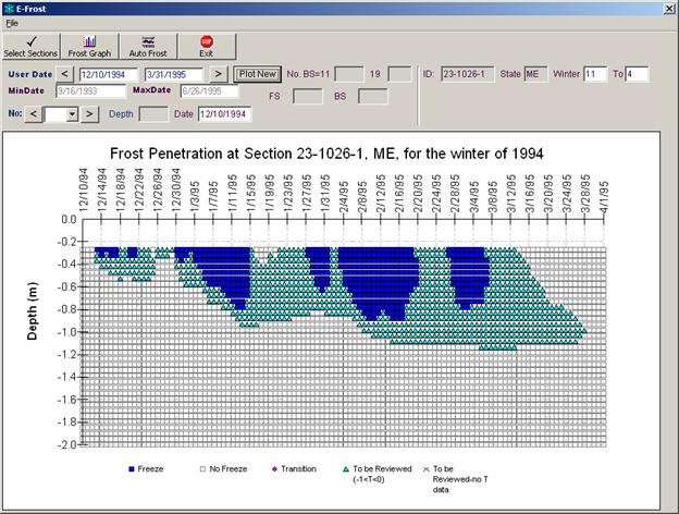
Figure 8. Chart. Frost predictions for section 1026 in Maine.

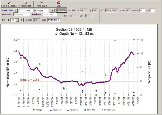
Figure 9. Chart. Comparison of ER, temperature and moisture trends for section 1026 in Maine.

ENHANCED INTEGRATED CLIMATIC MODEL

The Integrated Climatic Model (ICM) was developed in the late 1980s to simulate temporal variations in the temperature, moisture, and freeze-thaw conditions internal to the pavement and their impact on key pavement material properties.⁽¹⁴⁾ In FHWA-HRT-04-079,⁽¹⁷⁾ this program was recognized as the most comprehensive model addressing the effects of climate on pavements. As its name suggests, the EICM is an enhanced version of the ICM. It was used as the basis for considering seasonal variations in the Mechanistic-Empirical Pavement Design Guide (M-E PDG).

The EICM consists of three models addressing different aspects of climatic effects on the pavement:

• Climatic-Materials-Structures (CMS) model, developed at the University of Illinois. ⁽¹⁹⁾
• Infiltration and Drainage (ID) model, developed at the Texas Transportation Institute.⁽²⁰⁾
• Frost Heave and Thaw Settlement Model, developed by the CRREL.⁽²¹⁾

The EICM provides the capability to simulate temperature, moisture, and freeze-thaw conditions internal to the pavement structure as a function of time. The accuracy of the predictions depends greatly on a proper selection of boundary conditions, climatic parameters, and material properties.

The EICM engages a coupled heat moisture finite element/difference model. It models heat flow by considering climatic and solar inputs at the surface along with the deep ground constant heat source. These thermal boundary conditions are used in conjunction with the moisture content of the subpavement soils to model heat flow, the freezing state of the soil, and frost penetration accurately. The model is coupled in the sense that changes in moisture content affect the thermal properties of the unbound layers—an increase in the moisture content increases the heat capacity and thermal conductivity of the material. Moisture content in the unbound layer is affected by the thermal conditions when freezing occurs. The drying process in the unbound layer causes moisture to move to the freezing zone.

This tool could be particularly useful for modeling subsurface temperatures when temperature data are not available for some dates or depths.

Example Using EICM Model to Predict Missing Temperature

The EICM analysis algorithm provides enhanced options to fill in the gaps in partial or incomplete measured subsurface temperature data, including a temperature auto-correction option. The analysis starts with inputting pavement and unbound layer data from the LTPP database and historical climate measurements into the EICM program. After the initial program run, the EICM temperature predictions are compared to the measured temperature data. The detailed examination of the measured and predicted data gives further guidance on how the inputs can be refined. For example, the unbound materials may model as being wetter or drier than the initial inputs suggest. Adjustments to the moisture content present in the profile can be achieved by varying inputs into the soil water characteristic curves (SWCC) of each unbound layer or by adjusting the depth of the water table. These small refinements can bring the predicted and measured values into agreement.

The auto-correction option is used to further improve predictions. Using this option, the temperature profile for each SMP site is modeled and calibrated against available partial field measured data on a daily basis, with the initial temperature profile being the previous day's temperature reading. For each time step where temperature is known, the measured value will supersede and overwrite the predicted temperature, causing the measured and predicted temperatures to track exactly in line with one another.

When measured data are missing for a time period, the EICM model will start in perfect agreement with measured data at the beginning of the time period. As the model steps through time increments, it no longer has measured data to correct to, and the predicted output represents the only understanding of what the temperature is. However, because of the agreement that was achieved in the initial modeling and accurate initial profile (corrected by the measured data), the EICM is capable of accurately bridging short gaps in the data. When measured data are once again available, it is possible to observe the error in the prediction and again correct the predicted data with LTPP measured data. Figure 10 illustrates the comparison between the model predictions and the LTPP field data before auto-calibration, and figure 11 illustrates the comparison after auto-correction calibration.

Figure 10. Chart. Measured and EICM predicted temperatures for section 6251 in Minnesota at 0.8 m (2.6 ft) depth before auto-correction.

Figure 11. Chart. Measured and EICM predicted temperatures for section 6251 in Minnesota at 0.8 m (2.6 ft) depth after auto-correction.