U.S. Department of Transportation
Federal Highway Administration
1200 New Jersey Avenue, SE
Washington, DC 20590
202-366-4000
Federal Highway Administration Research and Technology
Coordinating, Developing, and Delivering Highway Transportation Innovations
 |
| This report is an archived publication and may contain dated technical, contact, and link information |
|
Publication Number: FHWA-HRT-08-057 Date: November 2008 |
Using the data analysis methodology presented in chapter 4, the existing FROST interactive procedure was updated to enhance the analysis algorithm, to address changes from SMP II experiment, and to assure compatibility with current database technology. The updated supporting research tool was named E-FROST to differentiate with the previous version.
The E-FROST research tool was developed to aid the data analyst in reviewing LTPP SMP data (temperature, ER, and moisture) and assigning freeze states based on the observed data trends. The primary functions of E-FROST are (1) to show time-series data from the in-situ measurements (ER, temperature, and moisture), (2) to generate and graphically represent frost penetration profiles, and (3) to create a frost penetration table containing frost penetration depths for different dates for which in-situ measurements were taken. The E-FROST user's guide with detailed instructions and examples is provided in appendix A.
Several improvements were made to the existing FROST interactive procedure to help determine the freeze state. To improve accuracy in frost penetration predictions in subsurface layers, the FROST algorithm was modified to include all available temperature, moisture, and ER data in the frost penetration analysis. The E-FROST graphic user interface was updated to provide means for review of daily temperature, moisture, and ER data plotted on the same plot. This feature enables the analyst to conduct comprehensive trend analysis of changes in temperature, ER, and moisture data in order to determine the freeze state of the soil at any date and depth that had in-situ measurements collected by LTPP.
The AutoFrost option was added to generate the initial frost penetration profile based on subsurface temperature values. This feature uses an objective measure, such as temperature at water freezing point, as a threshold value to determine the initial frost penetration profile instead of an arbitrary threshold value selected by the analyst, as was used in the previous FROST algorithm.
The EICM software was used for thermodynamic modeling of temperature distribution in subsurface layers, as appropriate, to fill the gaps in the field data and to aid the analyst in the examination of heat transfer processes based on the in-situ temperature data for the site. EICM-estimated subsurface temperature data was included in the E-FROST database so that it can be displayed on the interactive trend plots for the sites with missing or limited measured temperature data.
The original FROST program was developed to process data from the SMP I experiment. Introduction of the SMP II experiment led to the development of the new LTPP database tables to store ER data and resulted in a significant increase in the quantity of data to process for each site.
Introduction of the SMP II experiment also resulted in a different ER table structure and a significant increase of data to be processed for each SMP II site. E-FROST accounts for these changes. To cope with massive amounts of data, the program provides the analyst with options to review the data for the selected time intervals instead of displaying data for all dates on a single plot. The program routines and preprocessing database were updated to ensure database compatibility with Microsoft® Access 2000 or later, which is needed to facilitate preprocessing of the new SMP II data.
The decision tree algorithm for the E-FROST program is presented in figure 15.
Figure 15. Chart. Enhanced FROST algorithm.
Upon execution, E-FROST creates a temperature-based first order approximation of frost penetration profile for each SMP site using the AutoFrost analysis option. The profile consists of a grid with the horizontal axis displaying different SMP dates on a daily scale and the vertical axis displaying different analysis depth based on ER probe depths. Each cell is color-coded to provide information about the freeze state at a given date and given depth (see table 4).
| Color code | Symbol shape | Assigned freeze state | Subsurface temperature | Analyst's action |
|---|---|---|---|---|
Blue |
Rectangle | Freeze | T < -1 °C | Assigned automatically; however, the analyst has an option to change the state to transitional (pink) or no-freeze (white) upon data review |
White |
Rectangle | No freeze | T > 0 °C | Assigned automatically; however, the analyst has an option to change the state to transitional (pink) or freeze (blue) upon data review |
Light blue |
Triangle | Review | T < 0 °C and T > -1 °C | Assigned automatically; however, the action is required from analyst to manually review the data and change the state to freeze, no-freeze, or transitional |
Pink |
Diamond | Transitional | Near freezing isotherm | This color is assigned upon analyst review of all supporting data when it is not clear whether soil is frozen or not (partially frozen case) |
The E-FROST algorithm automatically assigns the state of subsurface freeze condition at each electrode location using the following rules:
Based on the assigned freeze state, different actions will be required. No actions are required for blue or white cells. If E-FROST assigns the cell as "Review" (light blue triangle), the analyst must review the data and change the freeze state as appropriate. To aid in this decision, E-FROST creates a time-series plot of ER, temperature, and moisture content changes. The plot appears on the screen once the analyst clicks on the light blue triangle cell. Similar plots can be brought up for review by clicking on any other cell on the frost penetration profile chart.
The following example demonstrates the frost penetration analysis procedure to determine the freeze state and layers for unbound pavement layers and subgrade for LTPP site 0804 in South Dakota. This site was chosen for the example because it contains the most comprehensive temperature, ER, and moisture data and provides means for cross-comparison of changes in all three measurement types. The plots provided in this example were generated using E-FROST.
ER, temperature, and moisture content data were obtained from the LTPP tables, which are specified in chapter 6. When measured subsurface temperatures were not available, temperature values were estimated using the EICM thermodynamic model; EICM inputs are listed in appendix B. An example of how temperature gaps could be filled out by EICM predictions using the thermodynamic model was shown in figure 11 (chapter 3).
Extracted LTPP data were preprocessed to obtain normalized ER values at calculated analysis depths and to interpolate temperature and moisture content data to those depths. Preprocessed electrical resistivity, temperature, and moisture content data were assembled in the analysis database table required to run E-FROST.
An automatic frost penetration profile was generated based on thermistor readings with the 0 °C isotherm used as a threshold value to differentiate freeze states. In the example shown in figure 16, all data points with temperature readings above 0 °C are shown using white squares with grey borders. These data points correspond to no-freeze states. All data points with temperature readings below -1 °C are shown using blue squares. These data points correspond to freeze states. Data points with temperature readings between data 0 °C and -1 °C are shown using light blue triangles. These data points require manual review, as they may represent a(n) frozen, unfrozen, or transitional state of soil.
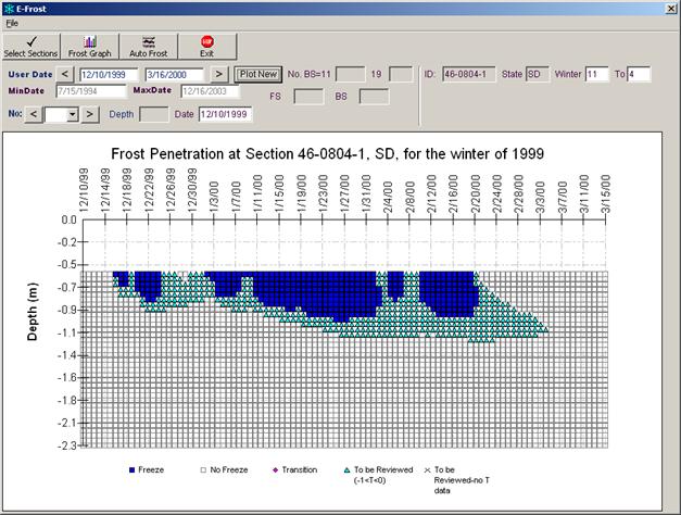
Figure 16. Chart. Example of temperature-based frost penetration profile for section 0804 in South Dakota.
Temperature, ER, and moisture content time-series trends were examined to verify the freeze state of soil assigned by the AutoFrost option, especially when temperatures were close to 0 °C. This was done by reviewing and correlating changes in temperature with changes in ER and moisture trends. E-FROST was used to graph temperature, ER, and moisture changes with time for each winter season and each measurement depth.
Upon data review, the state of soil was assigned to every date at every depth using trends described in table 3 as guidance. For the example shown in figure 17, the no-freeze state was assigned to dates prior to December 15 because the temperature readings, although close to 0 °C, never crossed the 0 axis. The state of the soil between December 16 and 24 was assigned as freeze as the data show a rapid drop in temperature values below 0 °C, followed by a decrease in moisture content. A transitional state of soil was assigned to December 25–27 and 30–31. Even though the temperature reading remained below 0 °C for these dates, there was a significant increase in moisture content, indicating thawing. The state of the soil for December 28 and 29 was assigned as no-freeze, as temperature values for these dates were above 0 °C. The state of the soil from January 1, 1999, to February 21, 2000, was assigned as freeze, as the trends in all three types of measurements (temperature, moisture, ER) indicated the possibility of frost—sharp decrease in moisture, sharp increase in ER, and temperature drop below 0 °C. For February 22, 2000, the no-freeze state was assigned based on observed trends in all three measurements: temperature rapidly rising above 0 °C, sharp decrease in ER, and sharp increase in moisture.
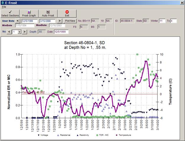
Figure 17. Chart. Example of ER, temperature, and moisture trends for section 0804 in South Dakota at 0.55 m (1.8 ft) depth.
Upon the completion of trend analysis at each of the 35 measurement depths and assignment of freeze states by the analyst, the E-FROST algorithm displays color-coded frost penetration profiles for review and quality assurance, as shown in figure 18.
Because of many less-than-ideal scenarios in the field data, the data interpretation process can be subjective. If the freezing condition at a particular point is in disagreement with the surrounding points (e.g., the point shows freezing while the soil above and below shows a no-freeze state), then the freeze state of that point may be changed by the analyst or QA reviewer to agree with that of the surrounding soil.
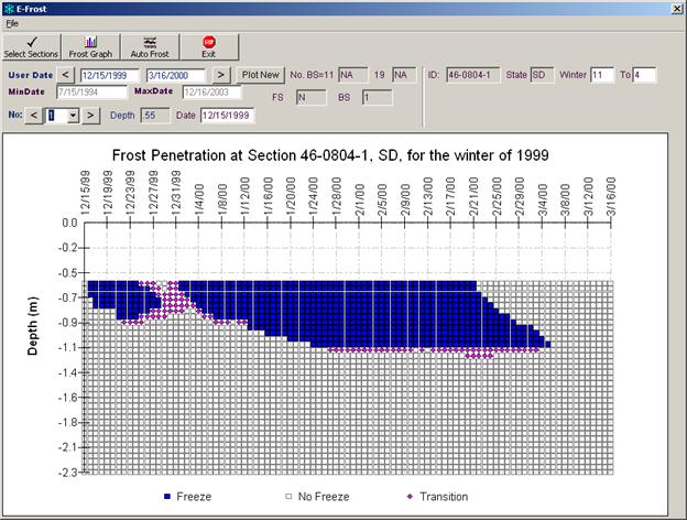
Figure 18. Chart. Example of final frost penetration profile for SMP site 46-0804 for the winter of 1999.
Using freeze state information at each measurement depth, frost depths were computed for each date using E-FROST. Frost depth calculations were based on the interpreted freeze states (F-frozen and T-transitional or partially frozen).
For each date, frost depths were computed based on the interpreted freeze states (F-frozen and T-transitional or partially frozen) using the following algorithm:
Freeze state information was added to SMP_FREEZE_STATE, and frost depth information was added to the SMP_FROST_PENETRATION table.
During temperature data analysis, there were multiple cases when temperatures were around 0 °C over a period of several days, pointing to a possibility of a transitional freeze state. However, these temperature trends were not consistently observed from one depth to another or for different years. Therefore, without supporting data (ER, moisture, soil salinity) or in cases of inconclusive supporting data trends, it was not possible to make definite conclusions whether or not the soil was in a transitional state.
Analysis of the sites that had similar temperature trends and had supporting ER and moisture data revealed that, although temperature values may indicate possible transitional state, low moisture and high ER values during the same period may provide evidence that soil may be in a freeze or no-freeze state. The following example demonstrates subjectivity of transitional state assignment based on temperature data alone. The temperature trend shown in figure 19 indicates the possibility of a transitional state of soil during the months of January and February 2001 based on temperatures just below 0 °C over an extended period of time. However, high ER values during the same period indicate that the state of soil is likely to be frozen. No moisture data are available for the same analysis period.
As a result of this limitation, the majority of freeze state estimates developed in this analysis study fall in either frozen or unfrozen categories. No transitional states were assigned based on the analysis of the temperature data alone, as that approach was found to be too subjective in absence of other supporting information (moisture, ER, soil salinity). When supporting ER and moisture data were available, a more detailed trend analysis was conducted resulting in a limited number of transitional state assignments.
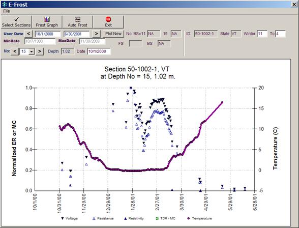
Figure 19. Chart. Temperature and ER trends at 1.02 m (3.35 ft) for site 50-1002 during winter season 2000–2001.
| << Previous | Contents | Next >> |

