U.S. Department of Transportation
Federal Highway Administration
1200 New Jersey Avenue, SE
Washington, DC 20590
202-366-4000
Federal Highway Administration Research and Technology
Coordinating, Developing, and Delivering Highway Transportation Innovations
| REPORT |
| This report is an archived publication and may contain dated technical, contact, and link information |
|
| Publication Number: FHWA-HRT-10-035 Date: September 2011 |
Publication Number: FHWA-HRT-10-035 Date: September 2011 |
To assess differences in the measured moduli determined from the AMPT and TP-62 protocols, a joint study was carried out between researchers at the Turner-Fairbank Highway Research Center (TFHRC) and NCSU. For this study, TFHRC performed dynamic modulus testing on a mixture following the AMPT TP, and NCSU performed testing on the same mixture using the TP-62 protocol.(8) In both cases, three replicates have been tested. To reduce any variability not related to the equipment and protocols, all specimens were fabricated at NCSU and randomly sampled for either AMPT testing or TP-62 testing. The details of each testing protocol are summarized in table 43.
| Factor | AMPT | TP-62 |
|---|---|---|
| Temperature (°F) | 40, 70, 100, and 130 | 14, 40, 70, 100, and 130 |
| Frequency (Hz) | 20, 10, 5, 1, 0.5, and 0.1 | 25, 10, 5, 1, 0.5, and 0.1 |
| Microstrain target | 75–125 | 50–75 |
| LVDT gauge length (mm) | 70 | 100 |
| Load direction | Bottom loading | Top loading |
| End treatment | Teflon® | Greased double latex membranes |
| Conditioning | External temperature chamber, then equalize in AMPT for 3 min | Equalize for 2.5–3.0 h in test machine |
| Rest period between frequencies (s) | 0 | 300 |
| Calculations | NCHRP 09-29 final 10 cycles(50) | NCHRP 09-29 final five cycles(50) |
|
°C = (°F−32)/1.8 |
||
The mixture used for this purpose is a 0.371-inch (9.5-mm) Superpave™ mixture typically used in North Carolina for surface courses. The gradation of this mixture is given in figure 133, and the relevant volumetric properties are summarized in table 44. All tests were conducted at 5.9 percent ±0.1 percent air void levels.
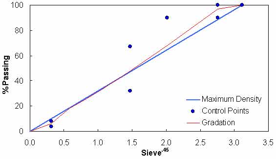
Figure 133. Graph. Test mixture gradation.
| Volumetric Property | Mix Design | Test Samples |
|---|---|---|
| Va (percent) | 3.8 | 5.9 |
| VMA (percent) | 15.6 | 17.5 |
| VFA (percent) | 75.7 | 66.2 |
| Asphalt content (percent) | 5.2 | 5.2 |
| Percent effective binder content | 4.9 | 4.9 |
| Dust percentage | 1.2 | 1.2 |
| Gmm | 2.616 | 2.616 |
| Bulk specific gravity of the aggregate | 2.828 | 2.828 |
| Effective specific gravity of the aggregate | 2.855 | 2.855 |
| Gb | 1.035 | 1.035 |
Results from the experimental study are summarized in figure 134 and figure 135, where the average dynamic moduli from the TP-62 protocol are plotted against the average moduli from the AMPT protocol. Error bars in these figures represent a single standard deviation from the mean. From these figures, it is observed that the AMPT test results are systematically lower than those from the TP-62 protocol; the difference between the two datasets is approximately 13 percent. Statistical analysis of these values using the step-down bootstrap method has also been performed. This method is used in lieu of multiple paired t-tests due to the effect of experimentwise error rates, which results in statistical errors when making multiple comparisons. Specifically, failing to account for this error rate increases the probability of finding significance when none is present. The statistical analysis results are shown by temperature and frequency in table 45. Note that in this table, the conditions under which the means are statistically similar are bold.
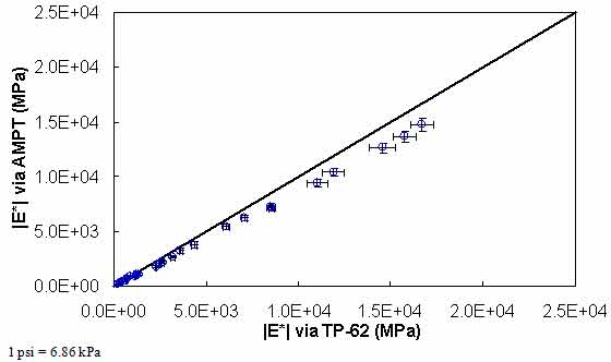
Figure 134. Graph. Comparison of |E*| measured via AMPT and TP-62 protocols in arithmetic scale.
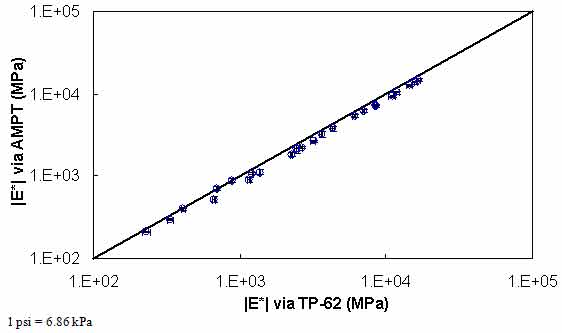
Figure 135. Graph. Comparison of |E*| measured via AMPT and TP-62 protocols in logarithmic scale.
| Temperature (°C) | Frequency (Hz) | |E*| AMPT (psi) | |E*| TP-62 (psi) | p-Value |
|---|---|---|---|---|
| 4 | 25.00 | 2,145,226 | 2,420,540 | 0.032 |
| 4 | 10.00 | 1,989,606 | 2,284,746 | 0.020 |
| 4 | 5.00 | 1,838,144 | 2,111,129 | 0.030 |
| 4 | 1.00 | 1,503,747 | 1,726,774 | 0.026 |
| 4 | 0.50 | 1,359,729 | 1,601,117 | 0.019 |
| 4 | 0.10 | 1,050,375 | 1,234,431 | 0.023 |
| 21 | 25.00 | 1,030,409 | 1,237,696 | 0.020 |
| 21 | 10.00 | 899,831 | 1,022,446 | 0.023 |
| 21 | 5.00 | 785,545 | 881,347 | 0.025 |
| 21 | 1.00 | 550,882 | 628,569 | 0.033 |
| 21 | 0.50 | 468,842 | 524,847 | 0.068 |
| 21 | 0.10 | 306,841 | 358,120 | 0.057 |
| 37 | 25.00 | 385,448 | 464,233 | 0.008 |
| 37 | 10.00 | 318,540 | 384,219 | 0.010 |
| 37 | 5.00 | 263,476 | 330,282 | 0.002 |
| 37 | 1.00 | 160,938 | 198,110 | 0.008 |
| 37 | 0.50 | 130,346 | 167,580 | 0.005 |
| 37 | 0.10 | 75,190 | 96,587 | 0.011 |
| 54 | 25.00 | 153,735 | 177,050 | 0.003 |
| 54 | 10.00 | 127,039 | 128,097 | 0.801 |
| 54 | 5.00 | 102,669 | 101,164 | 0.672 |
| 54 | 1.00 | 58,086 | 59,737 | 0.377 |
| 54 | 0.50 | 42,997 | 48,863 | 0.022 |
| 54 | 0.10 | 23,863 | 33,547 | 0.005 |
|
°C = (°F−32)/1.8 |
||||
To assess the differences observed between the two |E*| measurement protocols, a more comprehensive analysis was performed using the databases available in this study. The two AMPT and TP-62 databases were segregated based on the temperatures at which the |E*| values were measured. Because these two databases cover different ranges of parameters, it is useful to examine the distribution of the relevant parameters for the two databases. Figure 136 through figure 157 present the distribution and range of each parameter in the two databases. In figure 158 through figure 162, the measured |E*| data points available for some specific temperatures for each type of database are shown by frequency. Based on observations from these figures and the difference equation shown in equation 100, differences between the databases containing AMPT and TP-62 measurements are evident, as can be seen in table 46.
 |
(100) |
Based on this description, the following differences are observed at each temperature:
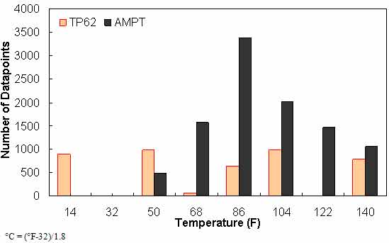
Figure 136. Graph. Frequency distribution of temperature in AMPT versus TP-62 databases.
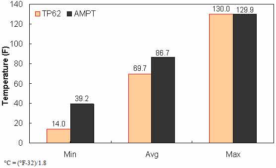
Figure 137. Graph. Range of temperature in AMPT versus TP-62 databases.
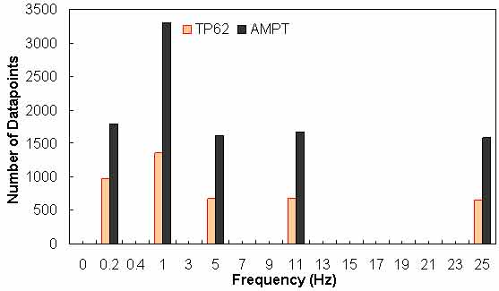
Figure 138. Graph. Frequency distribution of frequency in AMPT versus TP-62 databases.

Figure 139. Graph. Range of loading frequency in AMPT versus TP-62 databases.
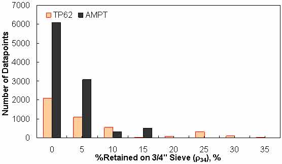
Figure 140. Graph. Frequency distribution of percentage retained on ¾-inch (19.05-mm) sieve (ρ34) in AMPT versus TP-62 databases.
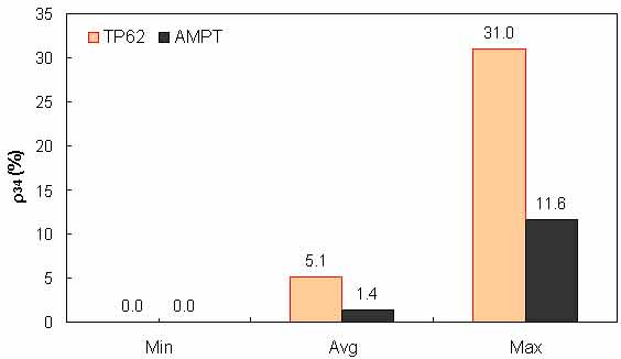
Figure 141. Graph. Range of percentage retained on ¾-inch (19.05-mm) sieve (ρ34) in AMPT versus TP-62 databases.
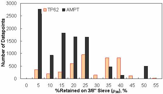
Figure 142. Graph. Frequency distribution of percentage retained on 3/8-inch (9.56-mm) sieve (ρ38) in AMPT versus TP-62 databases.
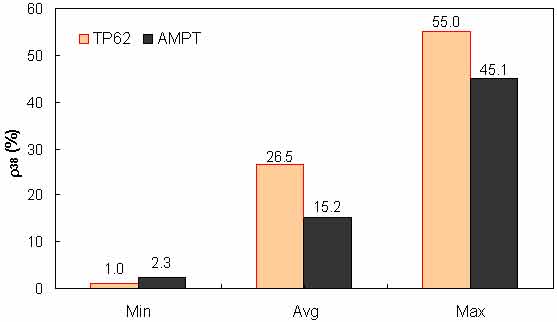
Figure 143. Graph. Range of percentage retained on 3/8-inch (9.56-mm) sieve (ρ38) in AMPT versus TP-62 databases.
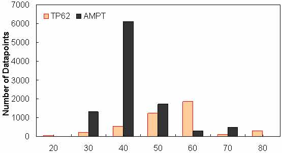
Figure 144. Graph. Frequency distribution of percentage retained on #4 sieve (ρ4) in AMPT versus TP-62 databases.
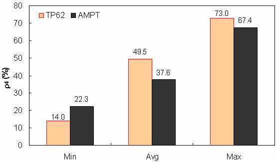
Figure 145. Graph. Range of percentage retained on #4 sieve (ρ4) in AMPT versus TP-62 databases.
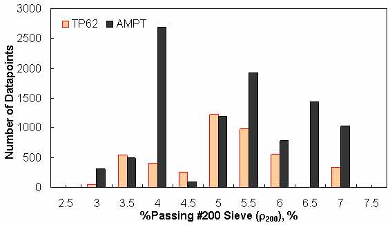
Figure 146. Graph. Frequency distribution of percentage passing #200 sieve (ρ200) in AMPT versus TP-62 databases.
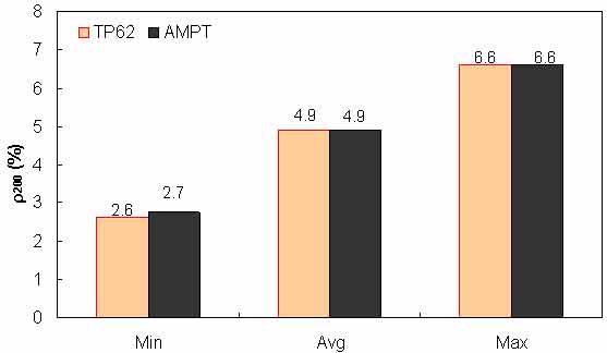
Figure 147. Graph. Range of percentage passing #200 sieve (ρ200) in AMPT versus TP-62 databases.
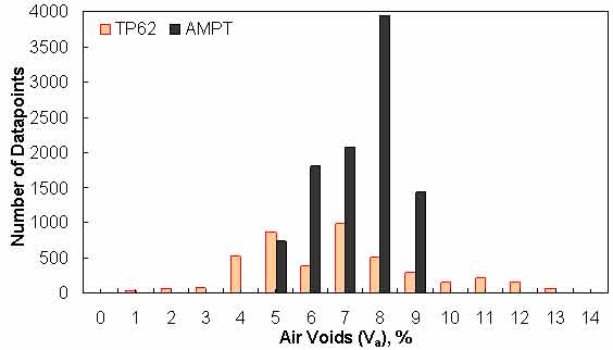
Figure 148. Graph. Frequency distribution of specimen air voids in AMPT versus TP-62 databases.
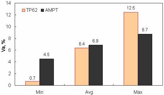
Figure 149. Graph. Range of specimen air voids in AMPT versus TP-62 databases.
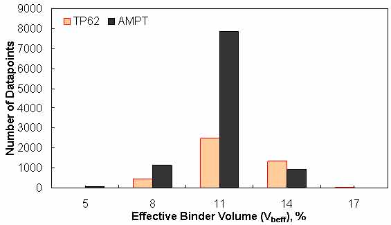
Figure 150. Graph. Frequency distribution of effective binder volume in AMPT versus TP-62 databases.
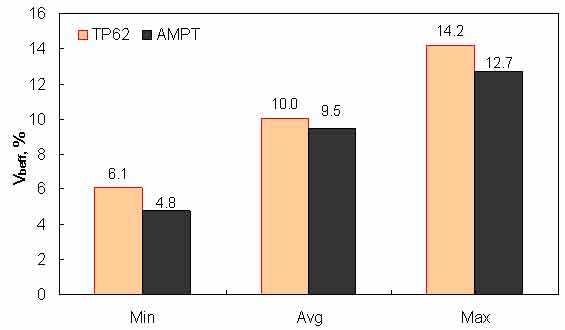
Figure 151. Graph. Range of effective binder volume in AMPT versus TP-62 databases.
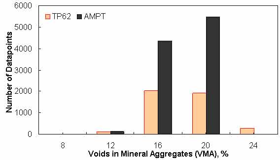
Figure 152. Graph. Frequency distribution of VMA in AMPT versus TP-62 databases.
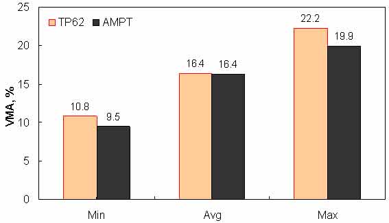
Figure 153. Graph. Range of VMA in AMPT versus TP-62 databases.
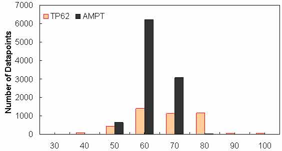
Figure 154. Graph. Frequency distribution of VFA in AMPT versus TP-62 databases.
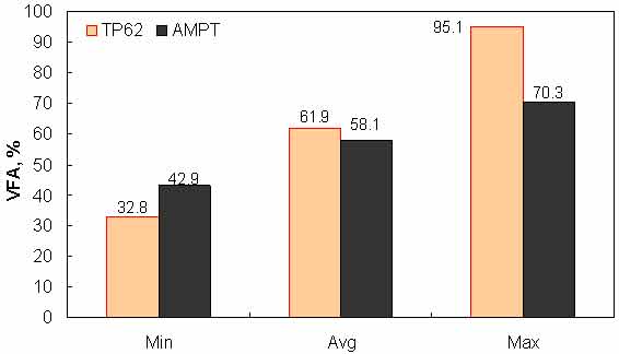
Figure 155. Graph. Range of VFA in AMPT versus TP-62 databases.
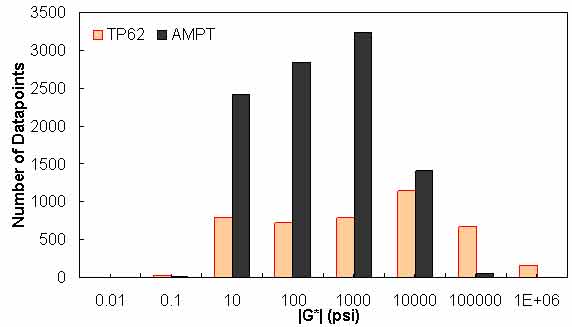
Figure 156. Graph. Frequency distribution of |G*| n AMPT versus TP-62 databases.
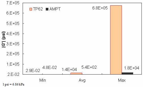
Figure 157. Range of |G*| in AMPT versus TP-62 databases.
Figure 158. Graph. Percentage of difference between AMPT versus TP-62 databases based on similar ranges of different variables at 39.9 °F (4.4 °C).
Figure 159. Graph. Percentage of difference between AMPT versus TP-62 databases based on similar ranges of different variables at 69.9 °F (21.1 °C).
Figure 160. Graph. Percentage of difference between AMPT versus TP-62 databases based on similar ranges of different variables at 100 °F (37.8 °C).
Figure 161. Graph. Percentage of difference between AMPT versus TP-62 databases based on similar ranges of different variables at 129.2 °F (54.0 °C).
Figure 162. Graph. Percentage of difference between AMPT versus TP-62 databases based on similar ranges of different variables at 129.9 °F (54.4 °C).
| Temp (°F) | 0 ≤ ρ34 ≤ 15 | 5 ≤ ρ38 ≤ 50 | 30 ≤ ρ4 ≤ 70 | 3 ≤ ρ200 ≤ 7 | 5 ≤ Va ≤ 9 | 8 ≤ Vbeff ≤ 14 | 12 ≤ VMA ≤ 20 | 50 ≤ VFA ≤ 80 | 1e-2 ≤ |G*| ≤ 1e5 |
|---|---|---|---|---|---|---|---|---|---|
| 40 | 46.08 | 39.80 | 41.14 | 43.54 | 42.75 | 45.65 | 44.81 | 44.29 | 43.60 |
| 70 | 59.39 | 47.54 | 51.74 | 57.66 | 57.67 | 60.23 | 59.91 | 58.32 | 57.84 |
| 100 | 62.63 | 49.53 | 51.35 | 61.61 | 63.38 | 64.49 | 64.36 | 62.66 | 61.95 |
| 129 | 45.60 | 51.02 | 49.65 | 46.26 | N.A | 63.01 | 46.16 | 52.09 | 46.26 |
| 130 | 57.55 | 40.76 | 44.14 | 57.46 | 60.50 | 59.99 | 60.54 | 57.93 | 57.83 |
|
°C = (°F−32)/1.8 |
|||||||||
Similar ranges of each variable have been considered for each temperature, and the percentage of error has been calculated based on the difference of average TP-62 versus AMPT |E*| measurements for the corresponding temperature.
A preliminary study was conducted to determine the feasibility and predictability of the ANN modeling technique relative to the existing models. This feasibility study was first conducted based on |G*| because more existing closed-form models use this parameter as their primary input parameter. The ANN models used in this preliminary study are not the final models suggested by the research team, but they are similar in form and validation. To ensure full coverage of the expected conditions, the most recent Witczak database with available measured |G*| data and a portion of the dataset obtained at NCSU with support from the NCDOT were utilized as the TP-62 training database. Also, appropriate portions of the FHWA mobile trailer database and the WRI database (from Kansas and Nevada sites) were considered as the AMPT training database (see table 47).(51,52) New parameters were not identified through this study. Instead, only those that have been used in the modified Witczak model are incorporated. For verification purposes, three different sets of independent databases were used (see table 48). As a corollary to this study, an additional ANN model was trained that uses the Hirsch model input parameters. The results from this model are given in this section, as well.
| Type of Database | AMPT | TP-62 | Total | ||
|---|---|---|---|---|---|
| FHWA I | WRI | Witczak | NCDOT I | ||
| Number of mixtures | 409 | 24 | 106 | 24 | 563 |
| Number of data points | 7,827 | 500 | 3,180 | 644 | 12,151 |
| Number of binders | 13 | 8 | 17 | 5 | 43 |
| Number of gradation variations | 13 | 12 | 13 | 19 | 57 |
| Number of volumetric variations | 256 | 13 | 98 | 24 | 391 |
|
Note: FHWA I consists of the mixtures from 12 States |
|||||
| Type of Database | AMPT | TP-62 | Total | |
|---|---|---|---|---|
| FHWA II | Citgo | NCDOT II | ||
| Number of mixtures | 84 | 8 | 12 | 104 |
| Number of data points | 1,652 | 168 | 338 | 2,158 |
| Number of binders | 3 | 2 | 3 | 8 |
| Number of gradation variations | 3 | 1 | 12 | 16 |
| Number of volumetric variations | 75 | 1 | 12 | 88 |
|
Note: FHWA II consists of the mixtures from three States in the FHWA mobile trailer database with the following site IDs: 1-IA0358, 2-WA0463, and 3-KS464. |
||||
It should be noted that the two TPs, AMPT and TP-62, were used to measure the |E*| values in the various databases. To illustrate any possible differences between the two protocols, three different ANNs were developed using the Witczak-based input parameters, as shown in table 49. G-GR pANN was trained using data from both the AMPT and TP-62 protocols, whereas AMPT pANN and TP-62 pANN models were trained using the data from AMPT only and TP-62 only. Table 49 summarizes the databases used to train and verify the ANNs.
| Model | Data Used in ANN Training | Description | Reference Scale | Statistical Parameters for Training Data | Statistical Parameters for Verification Data |
|||||
|---|---|---|---|---|---|---|---|---|---|---|
| AMPT | TP-62 | FHWA II | NCDOT II | Citgo | ||||||
| G-GR pANN | FHWA I | Witczak | ANNs trained with modified Witczak parameters | Arithmetic | Se/Sy = 0.29 R2 = 0.92 | Se/Sy = 0.38 R2 = 0.86 | Se/Sy = 0.33 R2 = 0.97 | Se/Sy = 0.52 R2 = 0.94 | ||
| WRI | NCDOT I | Log | Se/Sy = 0.15 R2 = 0.98 | Se/Sy = 0.35 R2 = 0.91 | Se/Sy = 0.27 R2 = 0.96 | Se/Sy = 0.59 R2 = 0.96 | ||||
| AMPT pANN | FHWA I | Arithmetic | Se/Sy = 0.24 R2 = 0.94 | Se/Sy = 0.36 R2 = 0.91 | Se/Sy = 0.63 R2 = 0.87 | Se/Sy = 0.37 R2 = 0.88 | ||||
| WRI | Log | Se/Sy = 0.16 R2 = 0.97 | Se/Sy = 0.38 R2 = 0.90 | Se/Sy = 0.60 R2 = 0.89 | Se/Sy = 0.48 R2 = 0.91 | |||||
| TP-62 pANN | Witczak | Arithmetic | Se/Sy = 0.34 R2 = 0.88 | Se/Sy = 2.08 R2 = 0.77 | Se/Sy = 0.24 R2 = 0.95 | Se/Sy = 1.20 R2 = 0.97 | ||||
| NCDOT I | Log | Se/Sy = 0.18 R2 = 0.97 | Se/Sy = 0.99 R2 = 0.82 | Se/Sy = 0.27 R2 = 0.93 | Se/Sy = 0.53 R2 = 0.99 | |||||
Modified Witczak Model |
Arithmetic | Se/Sy = 0.92 R2 = 0.91 | Se/Sy = 0.71 R2 = 0.91 | Se/Sy = 0.64 R2 = 0.98 | ||||||
| Log | Se/Sy = 0.58 R2 = 0.92 | Se/Sy = 0.19 R2 = 0.98 | Se/Sy = 0.26 R2 = 0.99 | |||||||
| Hirsch Model | Arithmetic | Se/Sy = 0.30 R2 = 0.92 | Se/Sy = 0.47 R2 = 0.97 | Se/Sy = 0.11 R2 = 0.99 | ||||||
| Log | Se/Sy = 0.39 R2 = 0.92 | Se/Sy = 0.26 R2 = 0.97 | Se/Sy = 0.09 R2 = 0.99 | |||||||
| Al-Khateeb Model | Arithmetic | Se/Sy = 0.48 R2 = 0.89 | Se/Sy = 0.55 R2 = 0.93 | Se/Sy = 0.36 R2 = 0.93 | ||||||
| Log | Se/Sy = 0.43 R2 = 0.92 | Se/Sy = 0.40 R2 = 0.93 | Se/Sy = 0.17 R2 = 0.97 | |||||||
| Note: Blank cells indicate information is not applicable. |
||||||||||
The ANN models perform well, as shown in figure 163 to figure 180, which display the prediction accuracies of the different models for the combined AMPT and TP-62 data (figure 163 to figure 168), TP-62 data only (figure 169 to figure 174), and AMPT data only (figure 175 to figure 180). Also, these three groups of figures show the prediction accuracies of the ANNs separately. In these three figures, the type of data (i.e., AMPT versus TP-62) used in the ANN training matches the type of data used in the verification (e.g., figure 163 shows the prediction accuracy of the G-GR pANN model trained with the combined AMPT and TP-62 data on the combined AMPT and TP-62 data, etc.). It is noted that the data used in these figures were not included in the ANN training.
Figure 181 through figure 204 further demonstrate the differences between the AMPT and the TP-62 data and their effect on the prediction accuracies of the different ANNs. FHWA II data used in figure 181 through figure 188 are obtained using the AMPT protocol. The TP-62 pANN model trained with the TP-62 data and the modified Witczak model overpredict the measured |E*| values. Figure 189 through figure 196 present the prediction results for the NCDOT II data, which were measured using the TP-62 protocol. These figures illustrate the opposite effect on the prediction bias, that is, the effect of using the TP-62 data in the ANN training and predicting the AMPT data. In this case, the AMPT pANN model, trained using the AMPT data, underpredicts the |E*| values. The G-GR pANN model provides a promising ANN-based |E*| model, and the TP-62 pANN model shows good predictions without any significant bias. With the exception of the Citgo dataset, the G-GR pANN model provides high goodness of fit and correlation, as seen in table 49. The promising feature of the G-GR pANN model is that it improves the bias of |E*| predictions, particularly at high and low temperatures. This new ANN model is more sensitive to, and thus more likely to capture, the changes in volumetric parameters than all the other existing predictive models.
The findings from figure 163 to figure 204 are summarized as follows:
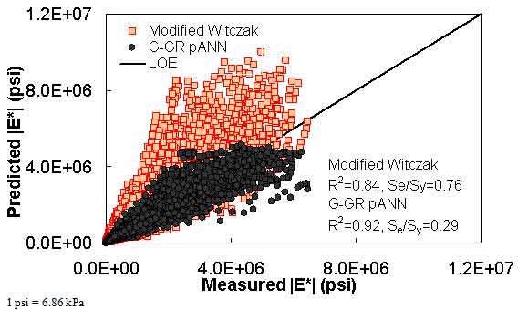
Figure 163. Graph. Prediction of the combination of AMPT and TP-62 data using the modified Witczak and G-GR pANN models in arithmetic scale.
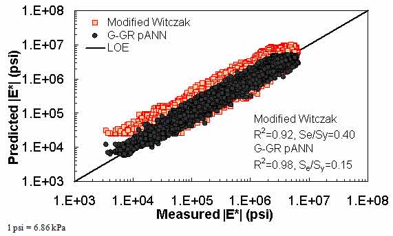
Figure 164. Graph. Prediction of the combination of AMPT and TP-62 data using the modified Witczak and G-GR pANN models in logarithmic scale.
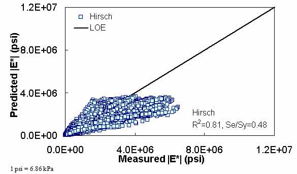
Figure 165. Graph. Prediction of the combination of AMPT and TP-62 data using the Hirsch model in arithmetic scale.
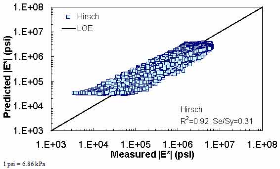
Figure 166. Graph. Prediction of the combination of AMPT and TP-62 data using the Hirsch model in logarithmic scale.
Figure 167. Graph. Prediction of the combination of AMPT and TP-62 data using the Al-Khateeb model in arithmetic scale.
Figure 168. Graph. Prediction of the combination of AMPT and TP-62 data using the Al-Khateeb model in logarithmic scale.
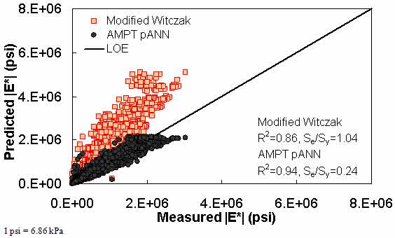
Figure 169. Graph. Prediction of the AMPT data using the modified Witczak and AMPT pANN models in arithmetic scale.
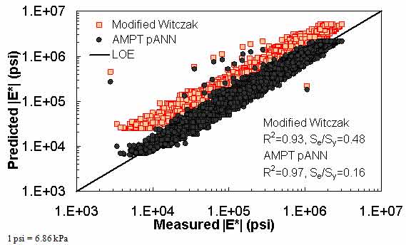
Figure 170. Graph. Prediction of the AMPT data using the modified Witczak and AMPT pANN models in logarithmic scale.
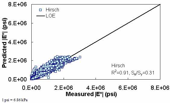
Figure 171. Graph. Prediction of the AMPT data using the Hirsch model in arithmetic scale.
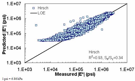
Figure 172. Graph. Prediction of the AMPT data using the Hirsch model in logarithmic scale.
Figure 173. Graph. Prediction of the AMPT data using the Al-Khateeb model in arithmetic scale.
Figure 174. Graph. Prediction of the AMPT data using the Al-Khateeb model in logarithmic scale.
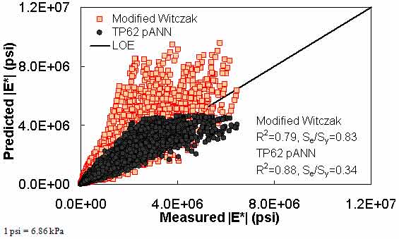
Figure 175. Graph. Prediction of the TP-62 data using the modified Witczak and TP-62 pANN models in arithmetic scale.
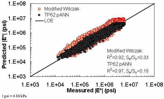
Figure 176. Graph. Prediction of the TP-62 data using the modified Witczak and TP-62 pANN models in logarithmic scale.
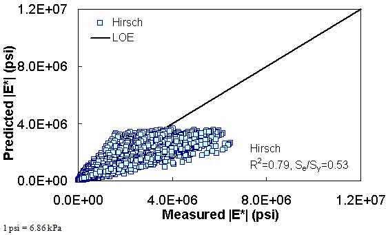
Figure 177. Graph. Prediction of the TP-62 data using the Hirsch model in arithmetic scale.
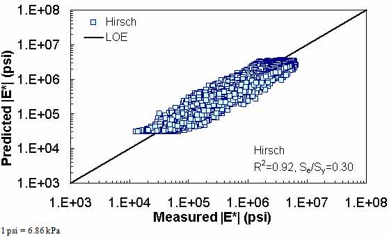
Figure 178. Graph. Prediction of the TP-62 data using the Hirsch model in logarithmic scale.
Figure 179. Graph. Prediction of the TP-62 data using the Al-Khateeb model in arithmetic scale.
Figure 180. Graph. Prediction of the TP-62 data using the Al-Khateeb model in logarithmic scale.
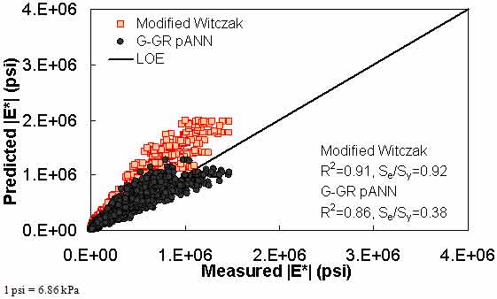
Figure 181. Graph. Prediction of the FHWA II data using the modified Witczak and G-GR pANN models in arithmetic scale.
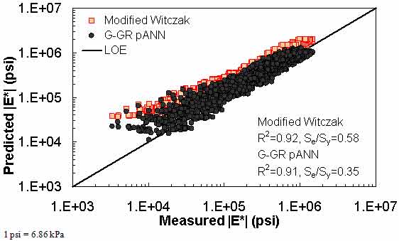
Figure 182. Graph. Prediction of the FHWA II data using the modified Witczak and G-GR pANN models in logarithmic scale.
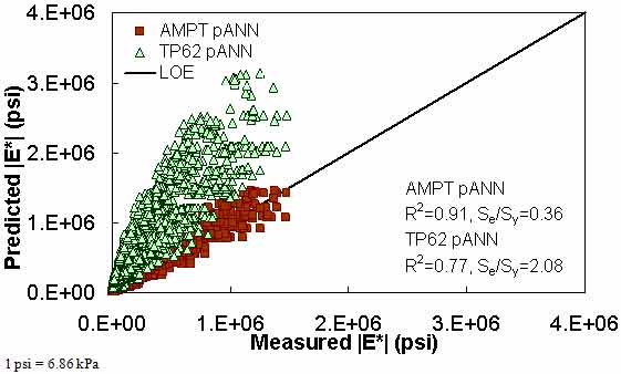
Figure 183. Graph. Prediction of the FHWA II data using the AMPT pANN and TP-62 pANN models in arithmetic scale.
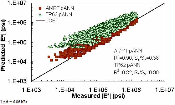
Figure 184. Graph. Prediction of the FHWA II data using the AMPT pANN and TP-62 pANN models in logarithmic scale.
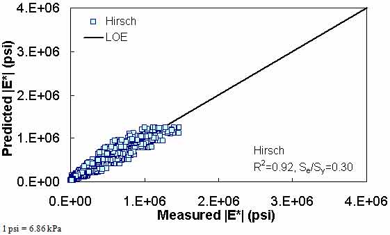
Figure 185. Graph. Prediction of the FHWA II data using the Hirsch model in arithmetic scale.
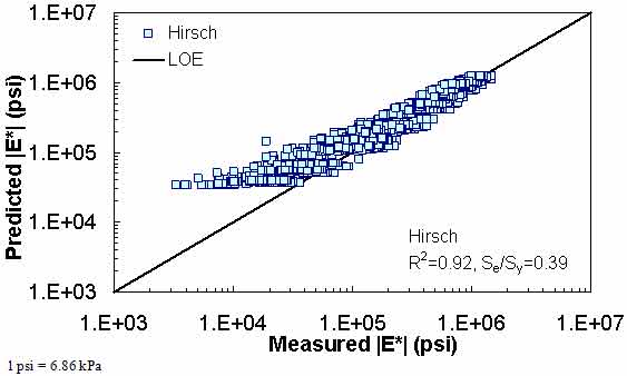
Figure 186. Graph. Prediction of the FHWA II data using the Hirsch model in logarithmic scale.
Figure 187. Graph. Prediction of the FHWA II data using the Al-Khateeb model in arithmetic scale.
Figure 188. Graph. Prediction of the FHWA II data using the Al-Khateeb model in logarithmic scale.
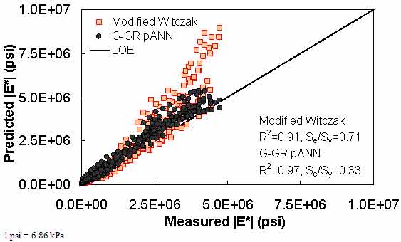
Figure 189. Graph. Prediction of the NCDOT II data using the modified Witczak and G-GR pANN models in arithmetic scale.
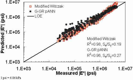
Figure 190. Graph. Prediction of the NCDOT II data using the modified Witczak and G-GR pANN models in logarithmic scale.
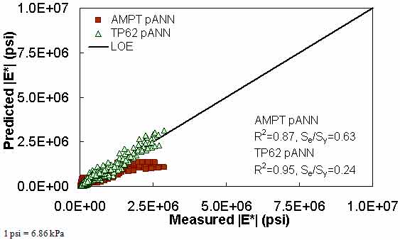
Figure 191. Graph. Prediction of the NCDOT II data using the AMPT pANN and TP-62 pANN models in arithmetic scale.
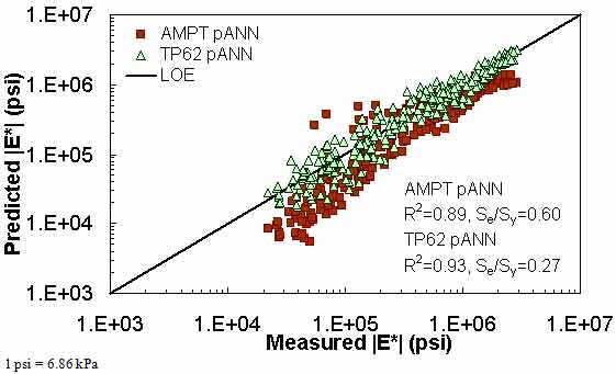
Figure 192. Graph. Prediction of the NCDOT II data using the AMPT pANN and TP-62 pANN models in logarithmic scale.
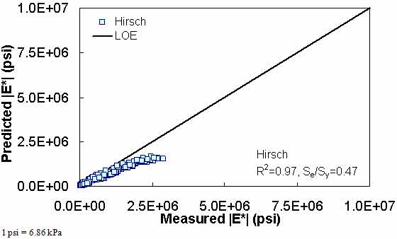
Figure 193. Graph. Prediction of the NCDOT II data using the Hirsch model in arithmetic scale.
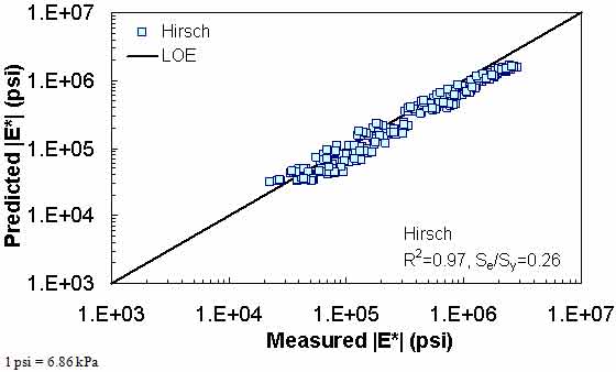
Figure 194. Graph. Prediction of the NCDOT II data using the Hirsch model in logarithmic scale.
Figure 195. Graph. Prediction of the NCDOT II data using the Al-Khateeb model in arithmetic scale.
Figure 196. Graph. Prediction of the NCDOT II data using the Al-Khateeb model in logarithmic scale.
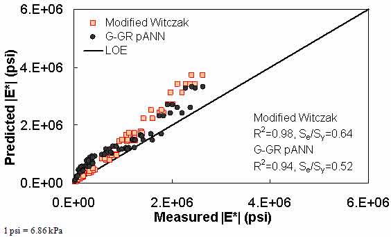
Figure 197. Graph. Prediction of the Citgo data using the modified Witczak and G-GR pANN models in arithmetic scale.
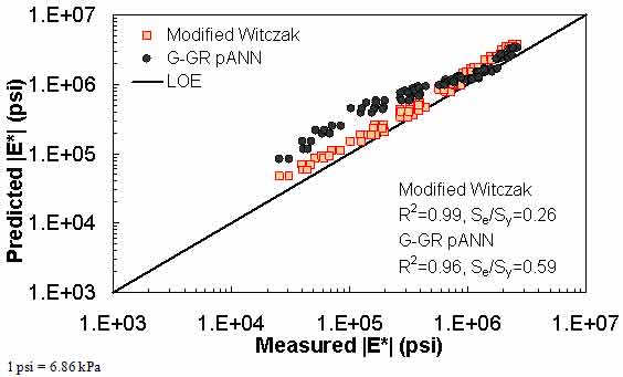
Figure 198. Graph. Prediction of the Citgo data using the modified Witczak and G-GR pANN models in logarithmic scale.
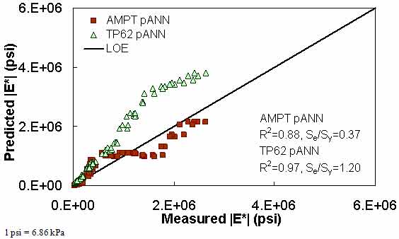
Figure 199. Graph. Prediction of the Citgo data using the AMPT pANN and TP-62 pANN models in arithmetic scale.
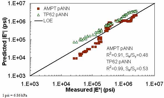
Figure 200. Graph. Prediction of the Citgo data using the AMPT pANN and TP-62 pANN models in logarithmic scale.
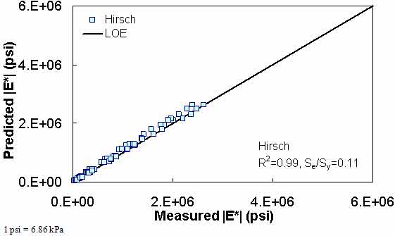
Figure 201. Graph. Prediction of the Citgo data using the Hirsch model in arithmetic scale.
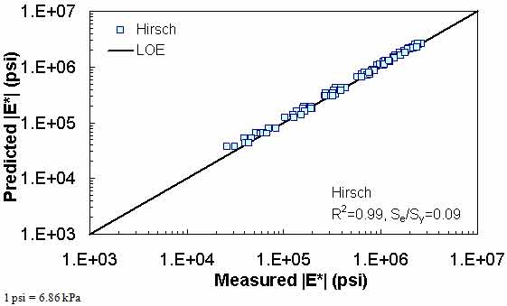
Figure 202. Graph. Prediction of the Citgo data using the Hirsch model in logarithmic scale.
Figure 203. Graph. Prediction of the Citgo data using the Al-Khateeb model in arithmetic scale.
Figure 204. Graph. Prediction of the Citgo data using the Al-Khateeb model in logarithmic scale.

