U.S. Department of Transportation
Federal Highway Administration
1200 New Jersey Avenue, SE
Washington, DC 20590
202-366-4000
Federal Highway Administration Research and Technology
Coordinating, Developing, and Delivering Highway Transportation Innovations
| REPORT |
| This report is an archived publication and may contain dated technical, contact, and link information |
|
| Publication Number: FHWA-HRT-10-066 Date: October 2011 |
Publication Number: FHWA-HRT-10-066 Date: October 2011 |
This chapter describes the analysis of rehabilitation alternatives for flexible pavements. The LTPP SPS-5 experiment was the main source of information for this study. The objective of the SPS-5 experiment, "Rehabilitation of Asphalt Concrete Pavements," was to help develop improved methodologies and strategies for the rehabilitation of flexible pavements. Specifically, the experiment evaluated common rehabilitation techniques implemented in the United States and Canada, and it evaluated the effects of climate, structural condition, and material variations on performance of rehabilitated flexible pavements. The design factorial is documented in Rehabilitation of Asphalt Concrete Pavements-Initial Evaluation of the SPS-5 Experiment, and included the following evaluation parameters:(4)
Variation of surface preparation alternatives, overlay material, and overlay thickness led to eight combinations at each SPS-5 project site (see table 32). In addition, one section was assigned as the control and did not receive any overlay, except for routine maintenance, creating nine experimental sections at each SPS-5 project site. As a result, each individual SPS-5 project provided a means for directly comparing rehabilitated HMA pavement performance using different surface preparation intensity, overlay thickness, and type of overlay mixture.
The initial SPS-5 sampling matrix was supposed to include only one subgrade type (fine-grained soil) with a minimum annual traffic of over 85,000 ESALs. Other factors considered in the sampling matrix included structural and functional condition of the pavement before overlay and climate. A total of 18 SPS-5 projects were constructed between 1989 and 1998. Table 33 presents the site location of each experiment according to their experimental design classification and as-built data. As shown, there were at least two projects for each condition except for the wet no-freeze fair condition cell and the dry freeze poor condition cell. A total of 162 test sections were built as part of the core SPS-5 experiment.
Table 32. Core sections of the SPS-5 experiment.
SHRP ID |
Overlay Type |
|---|---|
0501 |
Control: No treatment |
0502 |
Thin overlay (1.99 inches (51 mm)): Recycled HMA mix |
0503 |
Thick overlay (4.95 inches (127 mm)): Recycled HMA mix |
0504 |
Thick overlay: Virgin mix |
0505 |
Thin overlay: Virgin mix |
0506 |
Thin overlay: Virgin mix with milling |
0507 |
Thick overlay: Virgin mix with milling |
0508 |
Thick overlay: Recycled mix with milling |
0509 |
Thin overlay: Recycled mix with milling |
Table 33. Constructed SPS-5 sites for the experimental factorial.
Pavement Condition |
Soil Classification |
Climate, Moisture Temperature |
|||
|---|---|---|---|---|---|
Wet Freeze |
Wet |
Dry Freeze |
Dry |
||
Fair |
Coarse/fine |
Georgia |
Colorado |
||
Coarse |
New Jersey |
Alberta, Canada |
New Mexico |
||
Montana |
|||||
Fine |
Minnesota |
Oklahoma |
|||
Texas |
|||||
Poor |
Coarse/fine |
Manitoba, Canada |
California |
||
Coarse |
Maine |
Florida |
Arizona |
||
Alabama |
|||||
Fine |
Maryland |
Mississippi |
|||
Missouri |
|||||
Note: Blank cells indicate data are not available.
One major deviation from the original SPS-5 experimental plan was the subgrade soil type. Originally, the subgrade soils for all SPS-5 projects were supposed to be fine-grained soils; however, only five of the SPS-5 projects actually had fine-grained soils. Four SPS-5 projects had soils that varied between fine- and coarse-grained soils. The subgrade soils for the remaining eight SPS-5 projects were classified as coarse-grained soils.
Additionally, one major deviation from the original SPS-5 sampling matrix was subgrade soil type. Originally, the subgrade soils for all SPS-5 projects were supposed to be fine-grained soils. However, only six of the SPS-5 projects actually had fine-grained soils. Four SPS-5 projects had soils that varied between fine- and coarse-grained soils, while the remaining eight projects were classified as coarse-grained soils. Another deviation from the experimental plan for only a few of the SPS-5 projects was that no control section was left in place. For example, section 0501 for the Colorado project included the placement of a thin overlay during rehabilitation.
The impact of design features and site conditions on performance and response can be evaluated by looking at the trends in the survey data over time. Statistical tests can be used to verify if there are differences in these trends and if they can be associated with any of the design features in the experiment. Moreover, it is important to establish if any information on performance or response is reproduced in other sites or if they are associated with a particular site characteristic (e.g., climate, traffic, etc.). The best approach to achieve this objective is to consider every site and section available to statistically compare performance and response.
The SPS-5 experimental designed was balanced between design features intended for investigation. With few exceptions, out of 9 sections in each one of the 18 sites, there was 1 control section and 8 sections that combined equally thin and thick overlays with virgin and reclaimed asphalt pavement (RAP) mixes and milling and not milling prior to overlay. This provided an opportunity for a gradual statistical analysis in which information was gained by sequentially analyzing the data from each site first and complemented with a consolidated analysis. The consolidated analysis involved evaluating all sites and sections simultaneously in search of general trends and conclusions about pavement performance and its dependency on design features and site conditions. Figure 13 illustrates the statistical analysis process.
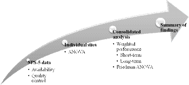
Figure 13. Illustration. Statistical analysis flow chart.
Statistical Approach and Tests
The approach consisted of analyzing each site individually to initially check its construction history to address possible problems during that phase. ANOVA was then used for repeated measures. ANOVA can be used to explain if different trends in performance exist because of a particular choice of design feature (e.g., milling versus no milling). The repeated measures are the surveys conducted throughout the duration of the experiment. Each section that is part of one site has the same site conditions and traffic volume. The surveys were performed within a short period for sections, which made ANOVA with repeated measures the best option for the statistical analysis of individual sites.
The consolidated analysis was performed using the Friedman test. This is a nonparametric test (distribution-free) used to compare repeated observations on similar subjects. Unlike the more common parametric repeated measures such as ANOVA or a paired t-test, the Friedman test makes no assumptions about the distribution of the data (e.g., normality), and it can be used for multiple comparisons. The Friedman test uses the ranks of the data rather than their raw values to calculate the statistic. The test statistic for the Friedman test is a chi-square with n - 1 degrees of freedom, where n is the number of repeated measures (i.e., the number of sections in each site of the experiment). Statistical significance was defined at 95 percent (p ≤ 0.05 for the chi-square test).
The Friedman test also permits the evaluation of paired statistical significance between two rehabilitation strategies. In some instances, the result of one analysis may indicate that significant differences exist between the rankings of sections (i.e., the performances of these sections are statistically different). However, there might be groups within the sorted ranking with similar performance. The paired statistical analysis feature is important to identify groups of strategies with equivalent performance.
The analysis of individual sites used distress and response data collected throughout the experiment duration. The data were checked for consistency and reasonableness prior to use in the analysis. Roughness, rutting, and fatigue, longitudinal, and transverse cracking were selected as indicative of performance and maximum deflection as indicative of response.
As described in the previous chapter, the consolidated analysis used WD as a performance measure of various distresses and the pavement response. It is calculated using the equation in figure 14.

Figure 14. Equation. Weighted distress.
The weighted average, in reality, represents the total normalized area (per year) under the distress versus time curve. As such, it is a measure of pavement performance relative to the specific distress over the entire monitoring period. The normalization to total time the section was in service provides means for comparing survey periods that may be different, which allowed the comparison of performance for both short term and long term.
The WD parameter is related to pavement performance over the whole analysis period. This concept is comparable to performance originally defined as the area under the serviceability curve.(2) The effect of variability from measurements by different surveyors is reduced when using this procedure and provided a parameter that could be used to compare sections with different survey periods. The WD performance measure proved a viable alternative to access the performance of different sections with individual in situ conditions and in-service ages. WD values were computed for the short term to evaluate performance in less than or equal to 5 years after rehabilitation was executed. Additionally, WD values were computed for the long term to compare performance for a period greater than 5 years.
The first task was to analyze the impact of design
features on performance for each site separately. The objective of this initial
step was to identify trends in performance that could be associated with each
design feature in the experiment (thin versus thick overlay, RAP versus virgin
mix, and milling versus no milling). ANOVA with repeated measures was the
statistical test used for this task. This statistical analysis took advantage of
the fact that all sections at each
SPS-5 site had the same underlying pavement structure, traffic, and climate. The
distress surveys and profile measurements were taken on the same day in all
sections within each site. The survey dates were used as the repeated measures
for the ANOVA.
The following section provides a complete example of the ANOVA tests used for the individual evaluation of SPS-5 sites. Each site in the experiment was evaluated following this sequential approach.
Example of Repeated Measures of ANOVA for Evaluation of SPS-5 Sites
Site Description and Data Availability
This site was assigned to LTPP in 1987, marking the initial data collection for the LTPP database. It is located at I-8 eastbound 17 mi (27.37 km) west of the I-10/I-8 interchange in Pinal County, AZ. The subgrade is a silty gravel soil with sand. The base course is a 14-inch (355-mm) soil aggregate mixture. The surface course is 5 inches (127 mm) of HMA. Traffic data are available since 1994, and AADTT for the LTPP lane is approximately 800 trucks. The average growth rate during the period is 8.5 percent. FHWA class 9 trucks account for 80 percent of the total truck traffic.
Data were available for all nine sections of this LTPP site. After being extracted from the LTPP database, performance data were evaluated for completeness and reasonableness. If any outliers were identified, they were removed from the analysis and recorded for reporting. In some instances, there were surveys performed on different days to cover all test sections in one specific date. When this happened, the missing survey was complemented with an interpolation of distresses measured during the previous and next survey dates. The reason for this was the need for equal numbers of surveys required to run ANOVA analysis with repeated measures.
All eight sections were rehabilitated in April 1990 following the selected SPS-5 experimental design. Section 0501 was used as the control section and was left without any rehabilitation. Data collection started after the rehabilitation and continued for 16 years until 2006. Data collection for the control section ended in 1993 probably as a result of the need to rehabilitate this section.
Analysis Approach
The analysis was performed for each type of distress previously described as well as for the maximum deflection. ANOVA with repeated measures was indicated in this case because the evaluation was carried out through a series of performance measurements taken throughout the duration of the experiment. The number of measurements in each section must be equal, and the experiment factorial must be balanced. The core sections of the SPS-5 experiment were balanced within each one of the three design features (overlay thickness, mix type, and surface preparation) and were independent. Without the control section, the eight remaining core sections provided an equal combination of all options in the design features. Therefore, the control section was not used for the statistical analysis of individual sites.
Repeated measures ANOVA is a technique used to test the equality of means. The null hypothesis has no differences between population means. The F-test in ANOVA evaluates the significance of the differences between means. A large F-value yields a correspondingly small p-value. The p-value is the observed significance level, or probability, of a type I error (alpha), which shows that the difference between population means exists when in fact there is no difference. In this study, an acceptable level of significance and probability of a type I error was defined as 0.05. The null hypothesis was rejected if the p-value was
Analysis of Performance
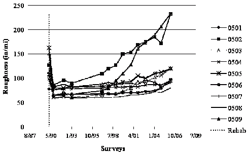
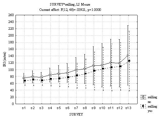
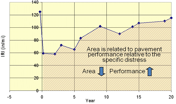
Roughness was measured by the IRI. Figure 15 presents an example showing IRI values for all sections in the site. The vertical dotted line indicates the year the sections were rehabilitated, as the measured roughness drops from the first to the second measurement. When the data were tested with the repeated measures ANOVA, they were grouped by different design features in the experiment.
1 inch = 25.4 mm
1 mi = 1.61 km
Figure 15. Graph. Roughness from an SPS-5 site in Arizona.
Figure 16 shows IRI over time for both thin and thick overlay sections. The marks are the average IRI for all sections grouped by overlay thickness. The bars represent the range of values with one standard deviation from the average. The p-value in the top of the chart is zero and indicates that there is a significant statistical difference in IRI values over time between sections with thin and thick overlays. The plot also indicates that sections with thick overlay performed better than those with thin overlays, as expected.
Statistically significant differences were also found when comparing sections overlaid with virgin versus recycled mixtures. Figure 17 shows IRI values over time for both mixture types, and the p-value was close to zero. The plot indicates that sections overlaid with virgin mix had better performance than those with recycled asphalt mix. It is interesting to note that soon after rehabilitation, IRI average values were not different between the two types of sections. The great significant difference in performance was more evident later in the pavements' service life.
Surface preparation prior to overlay did not have an
impact on roughness performance.
Figure 18 shows IRI values over time for sections that were milled versus not
milled prior to receiving the overlay. The p-value was close to 1.0 and
indicated that both distributions were statistically similar.
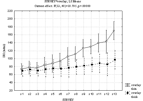
1 inch = 25.4 mm
1 mi = 1.61 km
Figure 16. Graph. IRI versus overlay thickness (distribution) for an SPS-5 site in Arizona.
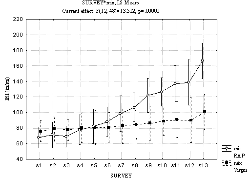
1 inch = 25.4 mm
1 mi = 1.61 km
Figure 17. Graph. IRI versus mix type (distribution) for an SPS-5 site in Arizona.
1 inch = 25.4 mm
1 mi = 1.61 km
Figure 18. Graph. IRI versus milling (distribution) for an SPS-5 site in Arizona.
The analysis of pavement performance associated with
roughness described previously was repeated for rutting, fatigue, longitudinal
cracking, and transverse cracking. The results are summarized in table 34. If a
statistically significant difference in performance existed, it is marked with
a "Y," and the corresponding design feature with the best performance was
indicated. When no difference was justified statistically, it is marked with an
"N" in the table.
In this case, a qualitative assessment was made of which design feature
provided the best performance. Blank cells indicate that no design feature had
predominant performance. For example, the first line (roughness) in table 34
indicates statistical differences in performance when evaluating the effect of
overlay thickness. In this case, for both short-term and long-term performances,
the performance for thick overlays (5-inch (127-mm)) was found to be better
than thin overlays (2-inch (51-mm)).
Table 34. Summary of statistical analysis results for SPS-5 site in Arizona.
Distress |
Overlay Thickness |
Mix Type |
Milling |
||||||
|---|---|---|---|---|---|---|---|---|---|
Statistical Difference |
Best Performance |
Statistical Difference |
Best Performance |
Statistical Difference |
Best Performance |
||||
Short |
Long |
Short |
Long |
Short |
Long |
||||
Roughness |
Y |
Thick |
Thick |
Y |
Virgin |
N |
Mill |
Mill |
|
Rutting |
Y |
Thin |
Thick |
Y |
Virgin |
Virgin |
N |
No mill |
|
Fatigue |
N |
Thick |
Thick |
N |
Y |
Mill |
Mill |
||
Transverse |
N |
N |
Virgin |
Virgin |
N |
||||
Longitudinal |
N |
Thin |
Y |
Virgin |
Virgin |
N |
|||
Note: Blank cells indicate that no
The repeated measures ANOVA results for this SPS-5 site suggest the following:
Conclusions from the Individual Analyses of SPS-5 Sites
The example presented in the previous section illustrates the approach taken to individually evaluate each site in the SPS-5 experiment. The summary tables for each site containing the results of the statistical analysis on performance for roughness, rutting, fatigue cracking, longitudinal cracking, and transverse cracking are presented in appendix A of this report.
The individual analysis of each site provided good qualitative information about the impact of design features on the performance of rehabilitated flexible pavement sections. The differences in performance are best visualized when compiled in plots that explore each design feature investigated in the SPS-5 experiment. These plots and key findings from the individual analyses of SPS-5 sites are presented in this section.
The compilation of results was created by identifying the number of sites in which various design features provided different performance throughout the site's service life. For example, if sections with thick overlays performed better than thin overlaid sections in one site, thick overlay was marked for the site. The process was repeated for all sites and distresses. The plots presented in this section summarize the percentage of sites in which differences in performance were identified. The number of sites with statistically justified differences from the ANOVA repeated measures test was also noted.
Results for roughness are provided in figure 19, suggesting that thick overlays provided the best performance in more than 50 percent of the sites. No differences in short-term performance were found in the majority of sites when comparing the two mix types. When long-term performance was evaluated, virgin mixes were found to perform better than recycled mixes, but no differences were found in 44 percent of sites. Milling improved performance in the majority of sites; however, one-third of sites had no differences in performance between milled and nonmilled sections.
The results in figure 19 were obtained from statistical analysis and engineering judgment when statistically significant differences were not found (p-values higher than 0.05) but differences in trends were clearly visible. The choice to consider both statistically-based and engineering judgment-based results was justified by the expansion of data analysis the two approaches provided combined. In the analysis of thickness, five sites (28 percent of all SPS-5 sites) had statistically significant differences in roughness performance. Four sites (22 percent) had statistically significant differences in the analysis of mix type, and three sites (17 percent) had statistically significant differences in the analysis of milling.
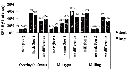
Figure 19. Graph. Summary of SPS-5 sites by best-performing design feature for roughness according to repeated measures ANOVA results.
Results for rutting are provided in figure 20, suggesting that the overlay thickness did not impact performance in the majority of sites. Mix type was also a design feature in which the impact on performance was not observed in the majority of sites. It is important to note that when differences were found, they were observed more in favor of sections overlaid with virgin mixes. The results also suggested that milling did not have an impact on rutting performance, and the majority of sites had milled and nonmilled sections performing similarly.
The results in figure 20 were obtained from statistical analysis and engineering judgment. Statistical significant differences were not found (p-values greater than 0.05), but differences in trends were clearly visible. In the analysis of thickness, five sites (28 percent of all SPS-5 sites) had statistically significant differences in rutting performance. Four sites (22 percent) had statistically significant differences in the analysis of mix type, and only two sites (12 percent) had statistically significant differences in the analysis of milling.
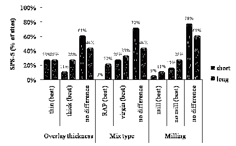
Figure 20. Graph. Summary of SPS-5 sites by best-performing design feature for rutting according to repeated measures ANOVA results.
Results for fatigue cracking are summarized in figure 21. None of the design features evaluated had an impact on short-term fatigue cracking performance. Sections with thick overlays had better long-term performances than thin overlays, although there were still 44 percent of sites in which no differences were found. Sections with virgin mix overlay had better long-term performances in half of the sites. Surprisingly, milled and nonmilled sections had equivalent long-term performances in the majority of sites.
The results in figure 21 were obtained from statistical analysis and engineering judgment. Statistically significant differences were not found (p-values higher than 0.05), but differences in trends were clearly visible. In the thickness analysis, four sites (22 percent of all SPS-5 sites) had statistically significant differences in fatigue cracking performance. Five sites (28 percent) had statistically significant differences in the analysis of mix type, and two sites (12 percent) had statistically significant differences in the analysis of milling.
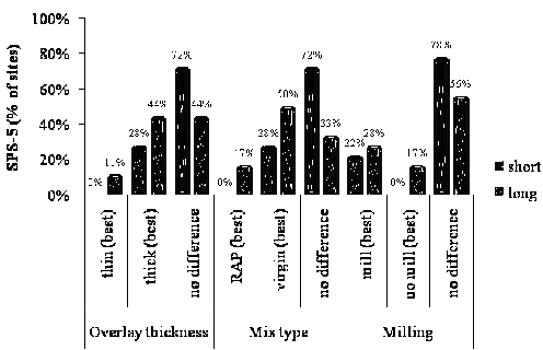
Figure 21. Graph. Summary of SPS-5 sites by best-performing design feature for fatigue cracking according to repeated measures ANOVA results.
Results for transverse cracking in figure 22 suggest that none of the design features evaluated in the SPS-5 experiment had any impact on performance in the majority of sites. It is worth noting that thick overlays had better transverse cracking long-term performance in 22 percent of sites, and milling prior to overlay had better transverse cracking long-term performance in 39 percent of sites.
The results in figure 22 were obtained from statistical analysis and engineering judgment. Statistically significant differences were not found (p-values greater than 0.05), but differences in trends were visible. In the thickness analysis, five sites (28 percent of all SPS-5 sites) had statistically significant differences in transverse cracking performance. Five sites (28 percent) had statistically significant differences in the analysis of mix type, and three sites (18 percent) had statistically significant differences in the analysis of milling.
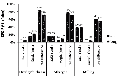
Figure 22. Graph. Summary of SPS-5 sites by best-performing design feature for transverse cracking according to repeated measures ANOVA results.
Results for longitudinal cracking are provided in figure 23 and suggest that for the majority of sites, none of the design features evaluated in the SPS-5 experiment had an impact on performance. It is worth noting that thin overlays had better longitudinal cracking long-term performance in 22 percent of sites, and milling prior to overlay had better longitudinal cracking long-term performance in 39 percent of sites.
The results in figure 23 were obtained from statistical analysis and engineering judgment. Statistically significant differences were not found (p-values greater than 0.05), but differences in trends were visible. In the thickness analysis, three sites (18 percent of all SPS-5 sites) had statistically significant differences in longitudinal cracking performance. Three sites (18 percent) had statistically significant differences in the mix type analysis, and four sites (22 percent) had statistically significant differences in the milling analysis.
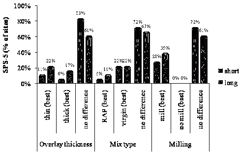
Figure 23. Graph. Summary of SPS-5 sites by best-performing design feature for longitudinal cracking according to repeated measures ANOVA results.
The key findings from the assessment of individual sites are listed below.
Roughness results were as follows:
Rutting results were as follows:
Fatigue cracking results were as follows:
Transverse cracking results were as follows:
Longitudinal cracking results were as follows:
The consolidated analysis involved compiling all sites in the SPS-5 experiment and simultaneously evaluating the impact of design features and site conditions for short-term and long-term performance. WD was the parameter selected for the comparisons, and it allowed the analysis to be carried across different conditions observed in each site of the experiment (more specifically, the different periods of monitoring data).
After the data were processed and verified for quality and existing outliers were corrected after LTPP analysis or removed, WD was computed for short-term and long-term performance. For simplicity, only the values for long-term performance are shown in table 35 through table 39. The remaining results are available in appendix A of this report. The Friedman test used the distress-associated WD to create a ranking of performance from the lowest value of WD (best performance) to the highest value (worst performance) for each site in the dataset. Ranking statistics for each type of section were then used to calculate the Friedman chi-square value used to determine if statistical differences existed among the performance rankings of the sections.
The WD-distress represents the overall performance of the section. It is better understood as an index computed based on the entire performance at a given period, as illustrated in figure 24. Therefore, it is intended for comparative analyses. The higher the WD value, the more distressed the pavement section is compared to sections with lower WD values.
1 inch = 25.4 mm
1 mi = 1.61 km
Figure 24. Graph. Example of WD-distress values in comparative performance analysis for IRI trend after rehab.
Table 35. Long-term average WD-IRI values for SPS-5 sites.
Section |
Experimental Design |
Sites (State Codes)/Average WD-IRI Values (m/km) |
|||||||||||||||||||
|---|---|---|---|---|---|---|---|---|---|---|---|---|---|---|---|---|---|---|---|---|---|
Mill |
Mix |
Thickness (mm) |
1 |
4 |
6 |
8 |
12 |
13 |
23 |
24 |
27 |
28 |
29 |
30 |
34 |
35 |
40 |
48 |
81 |
83 |
|
0501 |
No |
None |
80 |
108 |
70 |
92 |
97 |
193 |
88 |
130 |
134 |
39 |
113 |
127 |
98 |
||||||
0502 |
No |
RAP |
51 |
55 |
134 |
130 |
65 |
49 |
40 |
42 |
80 |
90 |
96 |
72 |
74 |
70 |
44 |
86 |
82 |
93 |
104 |
0503 |
No |
RAP |
127 |
53 |
77 |
75 |
50 |
49 |
40 |
54 |
71 |
87 |
114 |
62 |
62 |
45 |
33 |
66 |
76 |
89 |
69 |
0504 |
No |
Virgin |
127 |
57 |
82 |
74 |
56 |
42 |
40 |
56 |
86 |
95 |
87 |
71 |
48 |
51 |
37 |
70 |
93 |
101 |
71 |
0505 |
No |
Virgin |
51 |
58 |
92 |
102 |
55 |
36 |
40 |
45 |
90 |
101 |
110 |
69 |
57 |
57 |
39 |
64 |
95 |
83 |
107 |
0506 |
Yes |
Virgin |
51 |
48 |
71 |
81 |
87 |
32 |
36 |
52 |
59 |
92 |
101 |
69 |
56 |
51 |
37 |
66 |
90 |
72 |
117 |
0507 |
Yes |
Virgin |
127 |
56 |
88 |
73 |
65 |
37 |
39 |
55 |
63 |
72 |
83 |
83 |
61 |
52 |
42 |
62 |
83 |
93 |
59 |
0508 |
Yes |
RAP |
127 |
65 |
64 |
64 |
52 |
46 |
49 |
48 |
53 |
80 |
92 |
62 |
48 |
48 |
35 |
61 |
74 |
78 |
63 |
0509 |
Yes |
RAP |
51 |
55 |
115 |
142 |
62 |
37 |
40 |
60 |
76 |
87 |
108 |
84 |
62 |
49 |
37 |
64 |
78 |
94 |
84 |
1 inch = 25.4 mm
1 ft = 0.305 m
1 mi = 1.61 km
Note: Higher WD values indicate rougher pavement over time. The blank cells indicate
data are not available
Table 36. Long-term average WD-rutting values for SPS-5 sites.
Section |
Experimental Design |
Sites (State Codes)/Average WD-Rutting Values (mm) |
|||||||||||||||||||
|---|---|---|---|---|---|---|---|---|---|---|---|---|---|---|---|---|---|---|---|---|---|
Mill |
Mix |
Thickness (mm) |
1 |
4 |
6 |
8 |
12 |
13 |
23 |
24 |
27 |
28 |
29 |
30 |
34 |
35 |
40 |
48 |
81 |
83 |
|
0501 |
No |
None |
0.36 |
0.15 |
0.33 |
0.56 |
0.36 |
0.27 |
0.55 |
0.33 |
0.31 |
0.14 |
0.41 |
0.36 |
0.36 |
||||||
0502 |
No |
RAP |
51 |
0.10 |
0.19 |
0.16 |
0.13 |
0.16 |
0.13 |
0.27 |
0.17 |
0.10 |
0.36 |
0.14 |
0.17 |
0.11 |
0.12 |
0.11 |
0.23 |
0.25 |
0.14 |
0503 |
No |
RAP |
127 |
0.13 |
0.15 |
0.10 |
0.11 |
0.17 |
0.13 |
0.27 |
0.25 |
0.08 |
0.43 |
0.19 |
0.12 |
0.09 |
0.15 |
0.17 |
0.16 |
0.33 |
0.17 |
0504 |
No |
Virgin |
127 |
0.14 |
0.11 |
0.16 |
0.09 |
0.15 |
0.14 |
0.31 |
0.21 |
0.07 |
0.60 |
0.12 |
0.17 |
0.11 |
0.15 |
0.12 |
0.21 |
0.28 |
0.13 |
0505 |
No |
Virgin |
51 |
0.12 |
0.12 |
0.15 |
0.12 |
0.13 |
0.12 |
0.25 |
0.15 |
0.09 |
0.33 |
0.12 |
0.13 |
0.10 |
0.12 |
0.16 |
0.18 |
0.18 |
0.16 |
0506 |
Yes |
Virgin |
51 |
0.09 |
0.11 |
0.12 |
0.14 |
0.11 |
0.12 |
0.35 |
0.12 |
0.09 |
0.36 |
0.12 |
0.20 |
0.13 |
0.15 |
0.15 |
0.25 |
0.25 |
0.18 |
0507 |
Yes |
Virgin |
127 |
0.13 |
0.21 |
0.20 |
0.17 |
0.14 |
0.13 |
0.33 |
0.22 |
0.09 |
0.59 |
0.08 |
0.17 |
0.12 |
0.18 |
0.15 |
0.25 |
0.22 |
0.21 |
0508 |
Yes |
RAP |
127 |
0.21 |
0.14 |
0.11 |
0.13 |
0.16 |
0.12 |
0.32 |
0.19 |
0.08 |
0.56 |
0.17 |
0.11 |
0.10 |
0.16 |
0.11 |
0.18 |
0.23 |
0.22 |
0509 |
Yes |
RAP |
51 |
0.13 |
0.16 |
0.13 |
0.09 |
0.13 |
0.13 |
0.30 |
0.43 |
0.11 |
0.33 |
0.11 |
0.17 |
0.13 |
0.15 |
0.09 |
0.16 |
0.26 |
0.15 |
Table 37. Long-term average WD-fatigue cracking values for SPS-5 sites.
Section |
Experimental Design |
Sites (State Codes)/Average WD-Fatigue Cracking Values (m2) |
|||||||||||||||||||
|---|---|---|---|---|---|---|---|---|---|---|---|---|---|---|---|---|---|---|---|---|---|
Mill |
Mix |
Thickness (mm) |
1 |
4 |
6 |
8 |
12 |
13 |
23 |
24 |
27 |
28 |
29 |
30 |
34 |
35 |
40 |
48 |
81 |
83 |
|
0501 |
No |
None |
2,305 |
692 |
13 |
810 |
1 |
51 |
1,927 |
2,475 |
11 |
0 |
46 |
377 |
2,305 |
692 |
|||||
0502 |
No |
RAP |
51 |
2,566 |
966 |
38 |
0 |
0 |
25 |
0 |
458 |
0 |
1,263 |
463 |
1 |
1 |
3 |
1,480 |
916 |
2,566 |
966 |
0503 |
No |
RAP |
127 |
513 |
137 |
1 |
0 |
0 |
5 |
0 |
46 |
0 |
993 |
151 |
0 |
10 |
8 |
1,052 |
734 |
513 |
137 |
0504 |
No |
Virgin |
127 |
475 |
111 |
0 |
0 |
0 |
96 |
0 |
4 |
2 |
0 |
178 |
2 |
1 |
0 |
384 |
544 |
475 |
111 |
0505 |
No |
Virgin |
51 |
1,467 |
674 |
1 |
0 |
0 |
183 |
0 |
94 |
0 |
16 |
165 |
1 |
4 |
0 |
700 |
681 |
1,467 |
674 |
0506 |
Yes |
Virgin |
51 |
474 |
1,261 |
0 |
0 |
0 |
9 |
0 |
198 |
3 |
1 |
7 |
6 |
1 |
0 |
765 |
822 |
474 |
1261 |
0507 |
Yes |
Virgin |
127 |
528 |
840 |
0 |
1 |
0 |
0 |
0 |
0 |
108 |
0 |
45 |
4 |
1 |
5 |
273 |
489 |
528 |
840 |
0508 |
Yes |
RAP |
127 |
85 |
180 |
0 |
0 |
0 |
84 |
0 |
258 |
0 |
725 |
47 |
0 |
1 |
8 |
399 |
498 |
85 |
180 |
0509 |
Yes |
RAP |
51 |
2,204 |
16 |
0 |
1 |
0 |
0 |
0 |
705 |
2 |
1,511 |
650 |
2 |
0 |
29 |
1,272 |
1068 |
2,204 |
16 |
1 ft = 0.305 m
1 inch = 25.4 mm
Note: Higher WD values indicate increased cracking in the pavement over time. The
blank cells indicate data are not available.
Table 38. Long-term average WD-transverse cracking values for SPS-5 sites.
Section |
Experimental Design |
Sites (State Codes)/Average WD-Transverse Cracking Values (m) |
|||||||||||||||||||
|---|---|---|---|---|---|---|---|---|---|---|---|---|---|---|---|---|---|---|---|---|---|
Mill |
Mix |
Thickness (mm) |
1 |
4 |
6 |
8 |
12 |
13 |
23 |
24 |
27 |
28 |
29 |
30 |
34 |
35 |
40 |
48 |
81 |
83 |
|
0501 |
No |
None |
0 |
154 |
63 |
38 |
140 |
245 |
201 |
32 |
270 |
33 |
91 |
30 |
32 |
||||||
0502 |
No |
RAP |
51 |
110 |
87 |
153 |
69 |
5 |
0 |
0 |
134 |
262 |
96 |
0 |
26 |
199 |
47 |
62 |
220 |
96 |
188 |
0503 |
No |
RAP |
127 |
4 |
339 |
194 |
11 |
0 |
0 |
0 |
54 |
196 |
136 |
0 |
14 |
69 |
44 |
24 |
98 |
88 |
151 |
0504 |
No |
Virgin |
127 |
0 |
40 |
83 |
43 |
0 |
0 |
0 |
32 |
200 |
3 |
0 |
35 |
50 |
3 |
5 |
4 |
61 |
250 |
0505 |
No |
Virgin |
51 |
54 |
216 |
197 |
64 |
8 |
0 |
0 |
152 |
327 |
50 |
0 |
57 |
155 |
56 |
52 |
186 |
288 |
81 |
0506 |
Yes |
Virgin |
51 |
1 |
50 |
152 |
90 |
2 |
0 |
0 |
129 |
294 |
65 |
1 |
51 |
9 |
2 |
33 |
4 |
130 |
39 |
0507 |
Yes |
Virgin |
127 |
1 |
2 |
100 |
10 |
0 |
0 |
0 |
4 |
149 |
1 |
4 |
10 |
11 |
0 |
0 |
2 |
143 |
208 |
0508 |
Yes |
RAP |
127 |
1 |
207 |
257 |
9 |
0 |
0 |
0 |
59 |
217 |
80 |
0 |
10 |
51 |
2 |
0 |
73 |
54 |
225 |
0509 |
Yes |
RAP |
51 |
13 |
339 |
209 |
40 |
0 |
0 |
0 |
5 |
230 |
32 |
1 |
0 |
47 |
9 |
30 |
155 |
19 |
110 |
1 ft = 0.305 m
1 inch = 25.4 mm
Note: Higher WD values indicate increased cracking in the pavement over time. The
blank cells indicate data are not available.
Table 39. Long-term average WD-longitudinal cracking values for SPS-5 sites.
Section |
Experimental Design |
Sites (State Codes)/Average WD-Longitudinal Cracking Values (m) |
|||||||||||||||||||
|---|---|---|---|---|---|---|---|---|---|---|---|---|---|---|---|---|---|---|---|---|---|
Mill |
Mix |
Thickness (mm) |
1 |
4 |
6 |
8 |
12 |
13 |
23 |
24 |
27 |
28 |
29 |
30 |
34 |
35 |
40 |
48 |
81 |
83 |
|
0501 |
No |
None |
0 |
364 |
842 |
1,039 |
939 |
894 |
239 |
563 |
670 |
380 |
53 |
170 |
250 |
||||||
0502 |
No |
RAP |
51 |
95 |
47 |
268 |
722 |
2 |
304 |
277 |
795 |
843 |
209 |
52 |
377 |
862 |
405 |
252 |
797 |
575 |
741 |
0503 |
No |
RAP |
127 |
143 |
337 |
430 |
552 |
2 |
209 |
292 |
624 |
549 |
101 |
96 |
186 |
949 |
508 |
113 |
646 |
579 |
848 |
0504 |
No |
Virgin |
127 |
86 |
26 |
362 |
715 |
9 |
132 |
302 |
429 |
677 |
52 |
33 |
176 |
827 |
103 |
83 |
80 |
704 |
669 |
0505 |
No |
Virgin |
51 |
92 |
130 |
342 |
996 |
27 |
293 |
277 |
486 |
894 |
47 |
465 |
270 |
585 |
268 |
28 |
797 |
319 |
932 |
0506 |
Yes |
Virgin |
51 |
0 |
78 |
485 |
673 |
0 |
144 |
214 |
627 |
737 |
52 |
88 |
205 |
599 |
158 |
36 |
337 |
84 |
574 |
0507 |
Yes |
Virgin |
127 |
19 |
3 |
459 |
410 |
0 |
129 |
277 |
651 |
649 |
17 |
74 |
89 |
753 |
60 |
65 |
19 |
456 |
578 |
0508 |
Yes |
RAP |
127 |
69 |
285 |
497 |
152 |
73 |
135 |
218 |
745 |
369 |
170 |
116 |
266 |
926 |
559 |
0 |
631 |
578 |
921 |
0509 |
Yes |
RAP |
51 |
100 |
329 |
492 |
152 |
8 |
206 |
138 |
99 |
572 |
146 |
54 |
322 |
826 |
411 |
48 |
639 |
544 |
392 |
1 ft = 0.305 m
1 inch = 25.4 mm
Note: Higher WD values indicate increased cracking in the pavement over time. The
blank cells indicate data are not available.
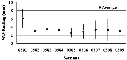
As noted earlier, the Friedman null hypothesis states that there are no differences between the ranking of sections (i.e., all sections have similar performances). The null hypothesis is rejected if the p-value is lower than 0.05, which represents a 95 percent confidence level that at least two sections have statistically different rankings. Examples of Friedman test outputs are provided in figure 25 and figure 26. In the figures, the average WD value for IRI found for each rehabilitation strategy among all sites was analyzed. The vertical bars represent the interval between the mean value ±1 standard deviation as an illustration of the variability of the measurements. The results in figure 25 indicate that for short-term roughness performance, there were at least two sections with statistically different performance (p < 0.0001, ANOVA chi-square = 48.8889). A similar result was found for long-term performance, as shown in figure 26 (p < 0.0001, ANOVA chi-square = 44.5667).

1 ft = 0.305 m
1 mi = 1.61 km
Figure 25. Graph. WD-IRI short-term values in SPS-5 sites.

1 ft = 0.305 m
1 mi = 1.61 km
Figure 26. Graph. WD-IRI long-term values in SPS-5 sites.
When the result of the Friedman test indicated the existence of at least two strategies with statistically different rankings, the next step was to identify which sections were different and to build the rankings of best-performing strategies based on the statistical analysis. Table 40 and table 41 provide the p-values for each Friedman test paired analysis for short-term and long-term roughness performance rankings.
Table 40. Friedman test paired analysis of rehabilitation strategies for short-term roughness performance ranking for SPS-5 sites.
Paired Analysis |
p-Value |
|---|---|
0501 and 0502 |
- |
0501 and 0503 |
< 0.05 |
0501 and 0504 |
< 0.05 |
0501 and 0505 |
- |
0501 and 0506 |
< 0.05 |
0501 and 0507 |
< 0.05 |
0501 and 0508 |
< 0.05 |
0501 and 0509 |
< 0.05 |
0502 and 0503 |
- |
0502 and 0504 |
- |
0502 and 0505 |
- |
0502 and 0506 |
- |
0502 and 0507 |
< 0.05 |
0502 and 0508 |
< 0.05 |
0502 and 0509 |
- |
0503 and 0504 |
- |
0503 and 0505 |
- |
0503 and 0506 |
- |
0503 and 0507 |
- |
0503 and  0508 |
- |
0503 and 0509 |
- |
0504 and 0505 |
- |
0504 and 0506 |
- |
0504 and 0507 |
- |
0504 and 0508 |
- |
0504 and 0509 |
- |
0505 and 0506 |
- |
0505 and 0507 |
- |
0505 and 0508 |
< 0.05 |
0505 and 0509 |
- |
0506 and 0507 |
- |
0506 and 0508 |
- |
0506 and 0509 |
- |
0507 and 0508 |
- |
0507 and 0509 |
- |
0508 and 0509 |
- |
- Indicates pair analysis with no
statistical significance.
Table 41. Friedman test paired analysis of rehabilitation strategies for long-term roughness performance ranking for SPS-5 sites.
Paired Analysis |
p-Value |
|---|---|
0501 and 0502 |
- |
0501 and 0503 |
< 0.05 |
0501 and 0504 |
- |
0501 and 0505 |
- |
0501 and 0506 |
< 0.05 |
0501 and 0507 |
< 0.05 |
0501 and 0508 |
< 0.05 |
0501 and 0509 |
- |
0502 and 0503 |
- |
0502 and 0504 |
- |
0502 and 0505 |
- |
0502 and 0506 |
- |
0502 and 0507 |
- |
0502 and 0508 |
< 0.05 |
0502 and 0509 |
- |
0503 and 0504 |
- |
0503 and 0505 |
- |
0503 and 0506 |
- |
0503 and 0507 |
- |
0503 and 0508 |
- |
0503 and 0509 |
- |
0504 and 0505 |
- |
0504 and 0506 |
- |
0504 and 0507 |
- |
0504 and 0508 |
- |
0504 and 0509 |
- |
0505 and 0506 |
- |
0505 and 0507 |
- |
0505 and 0508 |
- |
0505 and 0509 |
- |
0506 and 0507 |
- |
0506 and 0508 |
- |
0506 and 0509 |
- |
0507 and 0508 |
- |
0507 and 0509 |
- |
0508 and 0509 |
- |
- Indicates pair analysis with no
statistical significance.
The paired analysis results were used to create a practical ranking of roughness performance based on the statistical differences that were identified. The tables were intended to help users select the best alternatives given the specific conditions that they may want to evaluate. Based on the results presented in table 40 and table 41, the final ranking for evaluating roughness performance was created for the short term and long term (see table 42). Sections were ordered from best to worst performance, and sections with equivalent performance were grouped under the same rank.
Table 42. Ranking of rehabilitation strategies for roughness, SPS-5 sites.
Statistical Relevance (Y/N) |
Roughness |
|||
|---|---|---|---|---|
Short-Term |
Long-Term |
|||
Y |
(p < 0.0001) |
Y |
(p < 0.0001) |
|
Ranking |
Ranking |
Strategy |
Ranking |
Strategy |
1 |
Mill, thick, RAP |
1 |
Mill, thick, RAP |
|
2 |
Mill, thick, virgin |
2 |
No mill, thick, RAP |
|
3 |
No mill, thick, RAP |
2 |
Mill, thin, virgin |
|
3 |
No mill, thick, virgin |
2 |
Mill, thick, virgin |
|
3 |
Mill, thin, virgin |
5 |
No mill, thick, virgin |
|
3 |
Mill, thin, RAP |
5 |
Mill, thin, RAP |
|
3 |
No mill, thin, virgin |
5 |
No mill, thin, virgin |
|
8 |
No mill, thin, RAP |
8 |
No mill, thin, RAP |
|
9 |
Control |
9 |
Control |
|
The results in table 42 suggest that rehabilitations with milling and thick
recycled overlays provided smoother pavements in both the short-term and long-term
performance. Strategies with milling and virgin thick overlay were the second
best for short-term performance. For long-term roughness performance, three
strategies had equivalent second best performances. A broader analysis of both
rankings suggests that thick overlays provided better performance over the
short term and long term. Overall, differences between performance of recycled
asphalt and virgin overlays were difficult to identify, suggesting that roughness
performance was not significantly affected by the overlay mix type. Both
rankings also suggested that strategies with milling were more likely to
provide better short-term and long-term roughness performance. These results
agree with the conclusions drawn from the analysis of individual sites.
The same approach described for the analysis of roughness was applied to all distresses (rutting, fatigue, transverse, and longitudinal cracking). Figure 27 and figure 28 describe the Friedman test for rutting. Based on the same test statistics, the ranking of best-performing rehabilitation strategies for rutting was created (see table 43). The results suggest that thin overlays performed better at early stages for short-term performance (see figure 27, p < 0.0001, ANOVA chi-square = 40.2), while no significant differences were identified for long-term performance (see figure 28, p < 0.0001, ANOVA chi-square = 38.9778). The top rankings also were equally distributed among sections overlaid with virgin and RAP mixes and among sections previously milled and not milled. These findings agree with the observations from the analysis of individual sites.
1 inch = 25.4 mm
Figure 27. Graph. WD-rutting short-term values for SPS-5 sites.

1 inch = 25.4 mm
Figure 28. Graph. WD-rutting long-term values for SPS-5 sites.
Table 43. Ranking of rehabilitation strategies for rutting for SPS-5 sites.
Statistical Relevance (Y/N) |
Rutting |
|||
|---|---|---|---|---|
Short-Term |
Long-Term |
|||
Y |
(p < 0.0001) |
Y |
(p < 0.0001) |
|
Ranking |
Ranking |
Strategy |
Ranking |
Strategy |
1 |
No mill, thin, virgin |
1 |
No mill, thin, virgin |
|
1 |
No mill, thin, RAP |
1 |
Mill, thick, RAP |
|
1 |
Mill, thin, RAP |
1 |
No mill, thin, RAP |
|
1 |
Mill, thick, RAP |
1 |
Mill, thin, virgin |
|
1 |
Mill, thin, virgin |
1 |
No mill, thick, RAP |
|
1 |
No mill, thick, RAP |
1 |
Mill, thin, RAP |
|
1 |
No mill, thick, virgin |
1 |
No mill, thick, virgin |
|
8 |
Mill, thick, virgin |
8 |
Mill, thick, virgin |
|
9 |
Control |
9 |
Control |
|
Design features were found to have an impact on only long-term performance
associated with fatigue, longitudinal, and transverse cracking. Figure 29 through figure 31 present descriptive statistics for performance rankings
among all sites. Based on the Friedman test, the ranking of best-performing
rehabilitation strategies for cracking was created (see table 44 through table 46).
Figure 29 (p = 0.0009, ANOVA chi-square = 26.5074) and table 44 suggest
that thick overlays performed better in the long term for fatigue cracking. As
expected, it was evident from the figure that the no treatment control
alternative performed the poorest in regards to fatigue cracking. The ranking
of alternatives was more equally distributed when comparing mix types; however,
out of the top three alternatives, two were virgin mix overlays. Overall, mix
type had limited influence on long-term fatigue cracking performance. The
results also suggested that milling prior to overlay improved performance. Two
of the top three alternatives included milling prior to the overlay.
The results described in figure 30 (p < 0.0001, ANOVA chi-square = 33.6741) and table 45 suggested that thick overlays were better to mitigate transverse cracking. The two best-ranked sections had virgin mix overlays, but overall the performances of virgin and RAP mix overlays were similar. Sections that were milled prior to overlay consistently performed better than nonmilled ones.
The results for longitudinal cracking in figure 31 (p = 0.0011, ANOVA chi-square = 25.8407) and table 46 suggested that none of the design features had a significant influence on performance. Although the best alternative was milling and overlaying with a thick virgin mix, the remaining alternatives that ranked second consisted of different combinations of design features with no clear trend to which one provided better performance associated with longitudinal cracking.

1 ft2 = 0.093 m2
Figure 29. Graph. Fatigue cracking WD values for long-term performance of SPS-5 sites.

1 ft = 0.305 m
Figure 30. Graph. Transverse cracking WD values for long-term performance of SPS-5 sites.

1 ft = 0.305 m
Figure 31. Graph. Longitudinal cracking WD values for long-term performance of SPS-5 sites.
Table 44. Ranking of rehabilitation strategies for fatigue cracking at SPS-5 sites.
Statistical Relevance (Y/N) |
Long-Term |
|
|---|---|---|
Y |
p = 0.0009 |
|
Ranking |
Ranking |
Strategy |
1 |
No mill, thick, virgin |
|
1 |
Mill, thick, RAP |
|
1 |
Mill, thick, virgin |
|
4 |
Mill, thin, virgin |
|
4 |
No mill, thick, RAP |
|
4 |
No mill, thin, virgin |
|
4 |
Mill, thin, RAP |
|
4 |
No mill, thin, RAP |
|
9 |
Control |
|
Table 45. Ranking of rehabilitation strategies for transverse cracking at SPS-5 sites.
Statistical |
Long-Term |
|
|---|---|---|
Y |
p < 0.0001 |
|
Ranking |
Ranking |
Strategy |
1 |
Mill, thick, virgin |
|
2 |
No mill, thick, virgin |
|
3 |
Mill, thick, RAP |
|
3 |
Mill, thin, RAP |
|
3 |
Mill, thin, virgin |
|
3 |
No mill, thick, RAP |
|
7 |
No mill, thin, RAP |
|
8 |
No mill, thin, virgin |
|
8 |
Control |
|
Table 46. Ranking of rehabilitation strategies for longitudinal cracking at SPS-5 sites.
Statistical |
Long-Term |
|
|---|---|---|
Y |
p = 0.0011 |
|
Ranking |
Ranking |
Strategy |
1 |
Mill, thick, virgin |
|
2 |
Mill, thin, virgin |
|
2 |
No mill, thick, virgin |
|
2 |
Mill, thin, RAP |
|
2 |
No mill, thin, virgin |
|
2 |
Mill, thick, RAP |
|
7 |
No mill, thick, RAP |
|
7 |
Control |
|
7 |
No mill, thin, RAP |
|
The results obtained in the consolidated analysis agreed for the most part with the results found in the individual site analysis. Overlay thickness was the most influential design feature. Thick overlays consistently performed better, as expected. The impact of thickness on performance was more evident in the long term (more than 5 years) rather than the short term for most of the distresses used as performance measures. The exception was rutting, for which no evidence was found suggesting that either thin or thick overlays provided less rutted pavements.
The majority of sites did not show significant differences in performance between sections overlaid with virgin and RAP mixes. However, when differences existed, they were mostly in favor of virgin mixes.
The analysis of milling prior to overlay suggested that replacing the distressed portion of the surface layer improved the performance for the majority of distresses commonly observed in flexible pavements.
The influence of site condition was determined by three variables: (1) pavement surface condition prior to rehabilitation, (2) climate, and (3) traffic levels. These three conditions were determined for each site, and the Friedman test was repeated by grouping the sites according to each of the following variables:
The designation of fair versus poor was assigned by the owner agency nominating the SPS-5 project. These ratings were purely subjective and not based on the actual level of existing distresses prior to rehabilitation. They were used only to ensure a range of surface conditions of the original pavement before rehabilitation. However, the assessment of distresses prior to overlay indicated that, on average, fair pavements had IRI values of 9.50 ft/mi (1.8 m/km) with 0.39 inches (10 mm) or less of rutting and up to 1,237.86 ft2 (115 m2) of fatigue cracking per section. Poor pavements had roughness of 8.71 ft/mi (1.65 m/km) with 0.59 inches (15 mm) of rutting and up to 1,937.52 ft2 (180 m2) of fatigue cracking per section.
Climate condition was defined based on the freeze index and average rainfall for each site. Sites with an average annual rainfall greater than 39 inches (1,000 mm) were classified as wet, and sites with less than 39 inches (1,000 mm) of rain were classified as dry. Similarly, sites with a freeze index greater than 140 °F (60 °C) were classified as a freezing climate, and sites with less than 140 °F (60 °C) were designated as a no-freeze climate. These classifications are part of the LTPP experiment definition.
The classification of traffic was defined based on volume and commercial vehicle distribution. These characteristics were simple to evaluate and, at the same time, most influential on pavement performance predictions estimated with MEPDG. The combination of criteria generated two groups of sites: low traffic and high traffic. Table 47 describes the characteristics of both groups used in this study. Georgia and Texas did not have any traffic information.
Table 47. Criteria for evaluating traffic characteristics of SPS-5 sites.
Traffic Characteristics |
Low Traffic |
High Traffic |
|---|---|---|
AADTT |
340–950 |
750–2,750 |
Vehicle class 5 |
25–75 |
5–20 |
Vehicle class 9 |
10–50 |
40–85 |
SPS-5 sites |
Alabama, Florida, Maine, Maryland, Minnesota, Missouri, and Oklahoma |
Arizona, California, Colorado, Mississippi, Montana, New Jersey, New Mexico, Alberta, and Manitoba |
The analysis followed the same steps presented in the previous section. Rankings
of rehabilitation strategies were developed for each group of sites using
descriptive statistics and the paired analyses from the Friedman test when
statistical differences in performance were found. The results are summarized
in the tables presented in appendix C.
Table 48 and table 49 provide examples of how the data were summarized. These tables show the ranking of best-performing sections based on long-term performance for roughness and rutting in sections with fair and poor surface conditions prior to rehabilitation.
The examples illustrate the impact of site conditions on performance of rehabilitated flexible pavements. They suggest that rehabilitation strategies with milling and virgin mix overlays were better to improve roughness performance in pavements with poor surface condition. If surface condition was fair, RAP mixes provided a slight advantage in terms of roughness performance.
According to the ranking for rutting performance, rehabilitation strategies with milling and thin overlays with virgin mixes were the best alternatives when pavements had poor surface condition before the overlay. When surface conditions were fair, the impact of design features was not as significant. In fact, rehabilitation strategies with milling prior to overlay were among the worst ranked for rutting performance.
Table 48. Summary of rankings for long-term roughness and rutting performance of SPS-5 sites in fair surface condition prior to overlay.
Statistical Relevance (Y/N) |
Distress |
|||
|---|---|---|---|---|
Roughness |
Rutting |
|||
Y |
p = 0.0001 |
Y |
p = 0.0044 |
|
Ranking |
Ranking |
Strategy |
Ranking |
Strategy |
1 (Best) |
Mill, thick, RAP |
1 (Best) |
Mill, thick, RAP |
|
2 |
No mill, thick, RAP |
1 |
No mill, thin, virgin |
|
2 |
Mill, thin, virgin |
1 |
No mill, thick, RAP |
|
2 |
Mill, thin, RAP |
4 |
No mill, thick, virgin |
|
5 |
Mill, thick, virgin |
4 |
No mill, thin, RAP |
|
5 |
No mill, thick, virgin |
4 |
Mill, thin, RAP |
|
5 |
No mill, thin, virgin |
4 |
Mill, thin, virgin |
|
8 |
No mill, thin, RAP |
4 |
Mill, thick, virgin |
|
9 (Worst) |
Control |
9 (Worst) |
Control |
|
Table 49. Summary of rankings for long-term roughness and rutting performance of SPS-5 sites in poor surface condition prior to overlay.
Statistical Relevance (Y/N) |
Distress |
|||
|---|---|---|---|---|
Roughness |
Rutting |
|||
Y |
p = 0.019 |
Y |
p = 0.0015 |
|
Ranking |
Ranking |
Strategy |
Ranking |
Strategy |
1 |
Mill, thick, RAP |
1 |
No mill, thin, virgin |
|
2 |
Mill, thin, virgin |
1 |
Mill, thin, virgin |
|
2 |
Mill, thick, virgin |
3 |
Mill, thin, RAP |
|
2 |
No mill, thick, RAP |
3 |
No mill, thin, RAP |
|
2 |
No mill, thick, virgin |
3 |
No mill, thick, virgin |
|
2 |
No mill, thin, virgin |
3 |
No mill, thick, RAP |
|
2 |
No mill, thin, RAP |
3 |
Mill, thick, RAP |
|
2 |
Mill, thin, RAP |
3 |
Mill, thick, virgin |
|
9 |
None |
9 |
None |
|
A detailed assessment of the combined results for each of the analyses performed was assembled in tables for better visualization and interpretation of results. These tables were created for each distress and performance period (short-term and long-term performance) with the exception of fatigue and longitudinal cracking, which only presented statistically significant differences for long-term performance data . Table 50 and table 51 present the results for short-term and long-term roughness performance.
Table 52 and table 53 summarize the results for rutting. Table 54 shows the results for long-term fatigue cracking, and table 55 and table 56 present the results for short-term and long-term transverse cracking performance. Finally, table 57 summarizes the results for long-term longitudinal cracking. The best alternatives with statistical relevance are shown in each cell. The number before the treatment indicates its ranking among all alternatives.
The summary of best-performing strategies can be used as a practical guide to help select the best rehabilitation option based on performance. For example, if the section is located in a wet freeze region, and the pavement is in fair surface condition with low traffic levels, based on long-term roughness performance, three alternatives in table 51 provide equivalent best performance (mill, thick, and RAP; mill, thin, and virgin; and no mill, thick, and RAP). This performance-based selection can be further improved by evaluating material availability, costs, and other relevant issues.
These summary tables provide clear information for choosing the best rehabilitation treatment based on distress type and site condition. Moreover, the influence of different site conditions can be determined by observing the best treatments for each condition.
Table 50. Summary based on short-term roughness performance of SPS-5 pavement structures.
Climate |
Traffic/Surface Condition |
||||
|---|---|---|---|---|---|
High |
Low |
||||
Poor |
Fair |
Poor |
Fair |
||
Wet |
Freeze |
1: Mill, thick, virgin |
1: Mill, thick, virgin |
1: Mill, thick, virgin |
1: Mill, thick, virgin |
2: Mill, thick, RAP |
2: Mill, thick, RAP |
2: Mill thick, RAP |
2: Mill, thick, RAP |
||
3: No mill, thick, RAP |
3: No mill, thick, RAP |
3: No mill, thick, RAP |
2: No mill, thick, RAP |
||
4: Mill, thin, virgin |
4: Mill, thin, RAP |
4: Mill, thin, virgin |
4: Mill, thin, RAP |
||
No-freeze |
1: Mill, thick, virgin |
1: Mill, thick, virgin |
1: Mill, thick, virgin |
1: Mill, thick, virgin |
|
2: Mill, thick, RAP |
2: Mill thick, RAP |
2: Mill, thick, RAP |
2: Mill, thick, RAP |
||
3: Mill, thin, virgin |
3: No mill, thick, RAP |
3: No mill, thick, RAP |
3: No mill, thick, RAP |
||
3: No mill, thick, RAP |
4: Mill, thin, RAP |
4: Mill, thin, virgin |
4: Mill, thin, RAP |
||
Dry |
Freeze |
1: Mill, thick, RAP |
1: Mill, thick, RAP |
1: Mill, thick, RAP |
1: Mill, thick, RAP |
1: Mill, thick, virgin |
1: Mill, thick, virgin |
1: Mill, thick, virgin |
1: Mill, thick, virgin |
||
3: No mill, thick, RAP |
3: No mill, thick RAP |
3: No mill, thick, RAP |
3: No mill, thick, RAP |
||
- |
4: Mill, thin, RAP |
- |
4: Mill, thin, RAP |
||
No-freeze |
1: Mill, thick RAP |
1: Mill, thick, RAP |
1: Mill, thick, RAP |
1: Mill, thick, RAP |
|
1: Mill, thick, virgin |
1: Mill thick, virgin |
1: Mill, thick, virgin |
1: Mill, thick, virgin |
||
- |
3: Mill thin, RAP |
3: No mill, thick, RAP |
3: No mill, thick, RAP |
||
- |
3: No mill, thick, RAP |
- |
4: Mill, thin, RAP |
||
Indicates that no preferred treatment was statistically found.
Table 51. Summary based on long-term roughness performance of SPS-5 pavement structures.
Climate |
Traffic Surface/Condition |
||||
|---|---|---|---|---|---|
High |
Low |
||||
Poor |
Fair |
Poor |
Fair |
||
Wet |
Freeze |
1: Mill, thick, RAP |
1: Mill, thick, RAP |
1: Mill, thick, RAP |
1: Mill, thick, RAP |
1: Mill, thick, virgin |
1: Mill, thin, virgin |
1: Mill, thick, virgin |
1: Mill, thin, virgin |
||
1: Mill, thin, virgin |
1: No mill, thick, RAP |
1: Mill, thin, virgin |
1: No mill, thick, RAP |
||
1: No mill, thick, RAP |
4: Mill, thick, virgin |
1: No mill, thick, RAP |
4: Mill, thick, virgin |
||
No-freeze |
1: Mill, thick, RAP |
1: Mill, thick, RAP |
1: Mill, thick, RAP |
1: Mill, thick, RAP |
|
1: Mill, thick, virgin |
1: Mill, thin, virgin |
1: Mill, thick, virgin |
1: Mill, thin, virgin |
||
1: Mill, thin, virgin |
1: No mill, thick, RAP |
1: Mill, thin, virgin |
1: No mill, thick, RAP |
||
1: No mill, thick, RAP |
4: Mill, thick, virgin |
1: No mill, thick, RAP |
4: Mill, thick, virgin |
||
Dry |
Freeze |
1: Mill, thick, RAP |
1: Mill, thick, RAP |
1: Mill, thick, RAP |
1: Mill, thick, RAP |
1: No mill, thick, RAP |
1: No mill, thick, RAP |
1: No mill, thick, RAP |
1: No mill, thick, RAP |
||
3: Mill, thick, virgin |
3: Mill, thin, virgin |
3: Mill, thick, virgin |
3: Mill, thin, virgin |
||
3: Mill, thin, virgin |
4: Mill, thick, virgin |
3: Mill, thin, virgin |
4: Mill, thick, virgin |
||
No-freeze |
1: Mill, thick, RAP |
1: Mill, thick, RAP |
1: Mill, thick, RAP |
1: Mill, thick, RAP |
|
1: No mill, thick, RAP |
1: No mill, thick, RAP |
1: No mill, thick, RAP |
1: No mill, thick, RAP |
||
3: Mill, thick, virgin |
3: Mill, thin, virgin |
3:Mill, thick, virgin |
3: Mill, thin, virgin |
||
3: Mill, thin, virgin |
4: Mill, thick, virgin |
3: Mill, thin, virgin |
4: Mill, thick, virgin |
||
Table 52. Summary based on short-term rutting performance of SPS-5 pavement structures.
Climate |
Traffic Surface/Condition |
||||
|---|---|---|---|---|---|
High |
Low |
||||
Poor |
Fair |
Poor |
Fair |
||
Wet |
Freeze |
1: No mill, thin, virgin |
1:No mill, thin, RAP |
1: No mill, thin, virgin |
1: No mill, thin, virgin |
2: No mill, thin, RAP |
1: No mill, thin, virgin |
2: Mill, thin, virgin |
2: No mill, thin, RAP |
||
3: Mill, thick, RAP |
3: Mill, thick, RAP |
3: No mill, thin, RAP |
3: Mill, thick, RAP |
||
3: Mill, thin, virgin |
4: Mill, thin, RAP |
4: Mill, thick, RAP |
3: Mill, thin, RAP |
||
No-freeze |
1: No mill, thin, virgin |
1: No mill, thin, virgin |
1: Mill, thin, virgin |
1: No mill, thin, virgin |
|
2: Mill, thin, virgin |
2: No mill, thin, RAP |
1: No mill, thin, virgin |
2: Mill, thin, virgin |
||
3: No mill, thin, RAP |
3: Mill, thick, RAP |
3: Mill, thin, RAP |
3: Mill, thin, RAP |
||
4: Mill, thick, RAP |
3: Mill, thin, RAP |
3: No mill, thin, RAP |
3: No mill, thin, RAP |
||
Dry |
Freeze |
1: No mill, thin, virgin |
1: Mill, thick, RAP |
1: No mill, thin, virgin |
1: No mill, thin, virgin |
2: Mill, thick, RAP |
1: No mill, thin, RAP |
2: Mill, thick, RAP |
2: Mill, thick, RAP |
||
2: No mill, thin, RAP |
1: No mill, thin, virgin |
2: Mill, thin, RAP |
2: Mill, thin, RAP |
||
4: Mill, thin, RAP |
4: Mill, thin, RAP |
2: Mill, thin, virgin |
2: No mill, thick, RAP |
||
No-freeze |
1: No mill, thin, virgin |
1: No mill, thin, virgin |
1: No mill, thin, virgin |
1: No mill, thin, virgin |
|
2: Mill, thick, RAP |
2: Mill, thick, RAP |
2: Mill, thin, virgin |
2: Mill, thin, RAP |
||
2: Mill, thin, RAP |
2: Mill, thin, RAP |
3: Mill, thin, RAP |
3: Mill, thick, RAP |
||
2: Mill, thin, virgin |
2: No mill, thin, RAP |
4: Mill, thick, RAP |
3: Mill, thin, virgin |
||
Table 53. Summary based on long-term rutting performance of SPS-5 pavement structures.
Climate |
Traffic/Surface Condition |
||||
|---|---|---|---|---|---|
High |
Low |
||||
Poor |
Fair |
Poor |
Fair |
||
Wet |
Freeze |
1: No mill, thin, virgin |
1: No mill, thin, virgin |
1: No mill, thin, virgin |
1: No mill, thin, virgin |
2: Mill, thin, virgin |
2: Mill, thick, RAP |
2: Mill, thin, virgin |
2: Mill, thick, RAP |
||
3: Mill, thick, RAP |
2: No mill, thick, RAP |
3: Mill, thick, RAP |
2: Mill, thin, virgin |
||
3: No mill, thick, RAP |
4: Mill, thin, virgin |
3: No mill, thick, RAP |
2: No mill, thick, RAP |
||
No-freeze |
1: Mill, thin, virgin |
1: No mill, thin, virgin |
1: Mill, thin, virgin |
1: No mill, thin, virgin |
|
1: No mill, thin, virgin |
2: Mill, thin, virgin |
1: No mill, thin, virgin |
2: Mill, thin, virgin |
||
3: Mill, thin, RAP |
3: Mill, thick, RAP |
3: Mill, thin, RAP |
3: Mill, thick, RAP |
||
4: Mill, thick, RAP |
3: Mill, thin, RAP |
4: Mill, thick, RAP |
3: Mill, thin, RAP |
||
Dry |
Freeze |
1: No mill, thin, virgin |
1: Mill, thick, RAP |
1: No mill, thin, virgin |
1: No mill, thin, virgin |
2: Mill, thick, RAP |
1: No mill, thin, virgin |
2: Mill, thick, RAP |
2: Mill, thick, RAP |
||
2: No mill, thick, virgin |
3: No mill, thick, RAP |
2: Mill, thin, virgin |
3: No mill, thick, RAP |
||
4: Mill, thin, virgin |
3: No mill, thick, virgin |
2: No mill, thick, virgin |
3: No mill, thick, virgin |
||
No-freeze |
1: No mill, thin, virgin |
1:No mill, thin, virgin |
1: No mill, thin, virgin |
1: No mill, thin, virgin |
|
2: Mill, thin, virgin |
2: Mill, thick, RAP |
2: Mill, thin, virgin |
2: Mill, thick, RAP |
||
3: Mill, thick, RAP |
3: Mill, thin, RAP |
3: Mill, thick, RAP |
2: Mill, thin, virgin |
||
3: Mill, thin, RAP |
3: Mill, thin, virgin |
3: Mill, thin, RAP |
4: Mill, thin, RAP |
||
Table 54. Summary based on long-term fatigue cracking performance of SPS-5 pavement structures.
Climate |
Traffic Surface/Condition |
||||
|---|---|---|---|---|---|
High |
Low |
||||
Poor |
Fair |
Poor |
Fair |
||
Wet |
Freeze |
1: Mill, thick, virgin |
1: Mill, thick, virgin |
1: Mill, thick, virgin |
1: Mill, thick, virgin |
2: Mill, thick, RAP |
2: Mill, thick, RAP |
2: Mill, thick, RAP |
2: Mill, thick, RAP |
||
2: No mill, thick, virgin |
2: No mill, thick, virgin |
2: Mill, thin, virgin |
2: Mill, thin, virgin |
||
4: Mill, thin, virgin |
4: Mill, thin, virgin |
2: No mill, thick, RAP |
2: No mill, thick, RAP |
||
No-freeze |
1: Mill, thick, virgin |
1: Mill, thick, virgin |
1: Mill, thick, virgin |
1: Mill, thick, virgin |
|
2: Mill, thick, RAP |
2: Mill, thick, RAP |
2: Mill, thick, RAP |
2: Mill, thick, RAP |
||
2: No mill, thick, virgin |
2: No mill, thick, virgin |
2: Mill, thin, virgin |
2: Mill, thin, virgin |
||
4: Mill, thin, virgin |
4: Mill, thin, virgin |
2: No mill, thick, RAP |
2: No mill, thick, RAP |
||
Dry |
Freeze |
1: Mill, thick, RAP |
1: Mill, thick, RAP |
1: Mill, thick, RAP |
1: Mill, thick, RAP |
1: Mill, thick, virgin |
1: Mill, thick, virgin |
1: Mill, thick, virgin |
1: Mill, thick, virgin |
||
1: No mill, thick, virgin |
1: No mill, thick, virgin |
1: No mill, thick, virgin |
1: No mill, thick, virgin |
||
- |
- |
- |
- |
||
No-freeze |
1: Mill, thick, RAP |
1: Mill, thick, RAP |
1: Mill, thick, RAP |
1: Mill, thick, RAP |
|
1: Mill, thick, virgin |
1: Mill, thick, virgin |
1: Mill, thick, virgin |
1: Mill, thick, virgin |
||
1: No mill, thick, virgin |
1: No mill, thick, virgin |
1: No mill, thick, virgin |
1: No mill, thick, virgin |
||
4: Mill, thin, RAP |
4: Mill, thin, RAP |
4: Mill, thin, RAP |
4: Mill, thin, RAP |
||
- Indicates that no preferred treatment was statistically found.
Table 55. Summary based on short-term transverse cracking performance of SPS-5 pavement structures.
Climate |
Traffic/Surface Condition |
||||
|---|---|---|---|---|---|
High |
Low |
||||
Poor |
Fair |
Poor |
Fair |
||
Wet |
Freeze |
- |
- |
- |
- |
- |
- |
- |
- |
||
- |
- |
- |
- |
||
- |
- |
- |
- |
||
No-freeze |
1: Mill, thick, virgin |
1: Mill, thick, virgin |
1: Mill, thick, virgin |
1: Mill, thick, virgin |
|
1: No mill, thick, virgin |
1: No mill, thick, virgin |
1: No mill, thick, virgin |
1: No mill, thick, virgin |
||
- |
- |
- |
- |
||
- |
- |
- |
- |
||
Dry |
Freeze |
- |
- |
- |
- |
- |
- |
- |
- |
||
- |
- |
- |
- |
||
- |
- |
- |
- |
||
No-freeze |
1: Mill, thick, virgin |
1: Mill, thick, virgin |
1: Mill, thick, virgin |
1: Mill, thick, virgin |
|
1: No mill, thick, virgin |
1: No mill, thick, virgin |
1: No mill, thick, virgin |
1: No mill, thick, virgin |
||
- |
- |
- |
- |
||
- |
- |
- |
- |
||
- Indicates that no preferred treatment was statistically found.
Table 56. Summary based on long-term transverse cracking performance of SPS-5 pavement structures.
Climate |
Traffic/Surface Condition |
||||
|---|---|---|---|---|---|
High |
Low |
||||
Poor |
Fair |
Poor |
Fair |
||
Wet |
Freeze |
1: Mill, thick, virgin |
1: Mill, thick, virgin |
1: Mill, thick, virgin |
1: Mill, thick, virgin |
1: No mill, thick, virgin |
2: No mill, thick, virgin |
1: No mill, thick, virgin |
2: No mill, thick, virgin |
||
- |
3: Mill, thick, RAP |
3: Mill, thick, RAP |
3: Mill, thick, RAP |
||
- |
- |
3: No mill, thick, RAP |
4: No mill, thick, RAP |
||
No-freeze |
1: Mill, thick, virgin |
1: Mill, thick, virgin |
1: Mill, thick, virgin |
1: Mill, thick, virgin |
|
1: No mill, thick, virgin |
2: No mill, thick, virgin |
1: No mill, thick, virgin |
2: No mill, thick, virgin |
||
- |
3: Mill, thick, RAP |
3: Mill, thick, RAP |
3: Mill, thick, RAP |
||
- |
- |
3: No mill, thick, RAP |
4: No mill, thick, RAP |
||
Dry |
Freeze |
1: Mill, thick, virgin |
1: Mill, thick, virgin |
1: Mill, thick, virgin |
1: Mill, thick, virgin |
1: No mill, thick, virgin |
2: Mill, thick, RAP |
1: No mill, thick, virgin |
2: Mill, thick, RAP |
||
3: Mill, thick, RAP |
2: No mill, thick, virgin |
3: Mill, thick, RAP |
2: No mill, thick, virgin |
||
3: Mill, thin, RAP |
4: Mill, thin, RAP |
3: No mill, thick, RAP |
4: No mill, thick, RAP |
||
No-freeze |
1: Mill, thick, virgin |
1: Mill, thick, virgin |
1: Mill, thick, virgin |
1: Mill, thick, virgin |
|
1: No mill, thick, virgin |
2: No mill, thick, virgin |
1: No mill, thick, virgin |
2: No mill, thick, virgin |
||
3: Mill, thick, RAP |
3: Mill, thick, RAP |
3: Mill, thick, RAP |
3: Mill, thick, RAP |
||
3: Mill, thin, RAP |
4: Mill, thin, RAP |
3: No mill, thick, RAP |
4: No mill, thick, RAP |
||
- Indicates that no preferred treatment was statistically found.
Table 57. Summary based on long-term longitudinal cracking performance of SPS-5 pavement structures.
Climate |
Traffic/Surface Condition |
||||
|---|---|---|---|---|---|
High |
Low |
||||
Poor |
Fair |
Poor |
Fair |
||
Wet |
Freeze |
1: Mill, thick, virgin |
1: Mill, thick, virgin |
1: Mill, thick, virgin |
1: Mill, thick, virgin |
1: Mill, thin, virgin |
1: Mill, thin, virgin |
1: Mill, thin, virgin |
1: Mill, thin, virgin |
||
3: Mill, thick, RAP |
3: Mill, thick, RAP |
3: Mill, thick, RAP |
3: Mill, thick, RAP |
||
3: Mill, thin, RAP |
3: Mill, thin, RAP |
3: Mill, thin, RAP |
3: Mill, thin, RAP |
||
No-freeze |
1: Mill, thick, virgin |
1: Mill, thick, virgin |
1: Mill, thick, virgin |
1: Mill, thick, virgin |
|
1: Mill, thin, virgin |
1: Mill, thin, virgin |
1: Mill, thin, virgin |
1: Mill, thin, virgin |
||
3: Mill, thick, RAP |
3: Mill, thick, RAP |
3: Mill, thick, RAP |
3: Mill, thick, RAP |
||
3: Mill, thin, RAP |
3: Mill, thin, RAP |
3: Mill, thin, RAP |
3: Mill, thin, RAP |
||
Dry |
Freeze |
1: Mill, thick, RAP |
1: Mill, thick, virgin |
1: Mill, thick, RAP |
1: Mill, thick, virgin |
1: Mill, thick, virgin |
1: Mill, thin, virgin |
1: Mill, thick, virgin |
1: Mill, thin, virgin |
||
1: Mill, thin, RAP |
3: Mill, thick, RAP |
1: Mill, thin, RAP |
3: Mill, thick, RAP |
||
1: Mill, thin, virgin |
3: Mill, thin, RAP |
1: Mill, thin, virgin |
3: Mill, thin, RAP |
||
No-freeze |
1: Mill, thick, RAP |
1: Mill, thick, virgin |
1: Mill, thick, RAP |
1: Mill, thick, virgin |
|
1: Mill, thick, virgin |
1: Mill, thin, virgin |
1: Mill, thick, virgin |
1: Mill, thin, virgin |
||
1: Mill, thin, RAP |
3: Mill, thick, RAP |
1: Mill, thin, RAP |
3: Mill, thick, RAP |
||
1: Mill, thin, virgin |
3: Mill, thin, RAP |
1: Mill, thin, virgin |
3: Mill, thin, RAP |
||
The summary tables show only alternatives in which statistically significant differences in performance were identified with the Friedman test analysis. They were created by considering the best alternatives from each analysis performed in the dataset. These selected rehabilitation alternatives were then grouped for each combination of site conditions.
According to the summary tables, the following conclusions were made when roughness performance was considered:
The analysis of rutting indicated the following:
The analysis of fatigue cracking indicated the following:
The analysis of transverse cracking indicated the following:
The analysis of longitudinal cracking indicated the following:
The summary tables presented in this section, along with a complete set of tables with descriptive statistics for all the analyses conducted, are provided in appendix C.
Effect of Design and Contruction Features and Site Conditions on Response of Rehabilitated Flexible Pavements
The study to evaluate the impact of design features and site conditions on response of rehabilitated flexible pavements followed the same approach used in the analysis of performance. FWD deflection data are available in the LTPP database and used as the response measure of the pavement structure. Deflections in the wheel path of the LTPP lane were used as indicators of structural response.
The same analysis sequence applied to the study of performance was applied to the study of response. The first task was to evaluate individual sites and how the pavement structural responses were affected by each rehabilitation strategy and its design features. Since the analysis was carried out for each site separately, the deflection values were not adjusted for temperature, and the FWD survey was assumed to take place under similar conditions for all sections of a given site. There were small variations in surface temperature throughout the day, but they were considered minor and unlikely to significantly affect the total pavement stiffness. The variation of deflections over time and over the seasons throughout the year was used as input for the repeated ANOVA.
Individual Analysis of SPS-5 Sites
Summary tables containing the results of the statistical analysis for pavement response for each site are presented in appendix A.
A compilation of results was created by identifying the number of sites in which design features had provided differences in response throughout the site's service life. For example, if sections with thick overlays had lower deflection measurements than thin overlay sections in one site, the thick overlay was marked for this site, and the process was repeated for all sites. Figure 32 summarizes the percentage of sites in which differences in response were identified.
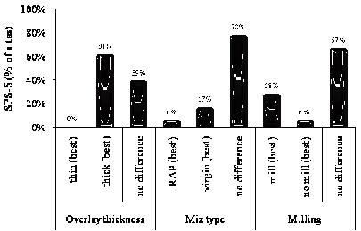
Figure 32. Graph. Percentage of SPS-5 sections with lower maximum deflection based on repeated measures ANOVA results.
The key findings from the assessment of individual sites were as follows:
The consolidated analysis involved the simultaneous analysis
of all sites in the SPS-5 experiment using the Friedman test. A follow-up
analysis was performed by grouping the data by site condition to evaluate the
impact of design features and site conditions for short-term and
long-term performance. WD was the parameter used for this analysis.
After the data were processed and verified for quality, WD was computed for each section in each SPS-5 site. The values are shown in table 58. The Friedman test used WD to create the ranking of performance from the lowest to the highest value for each site in the dataset. Ranking statistics for each type of section were then used to calculate the chi-square value, and this parameter was used to determine if statistical differences existed among the performance rankings of the sections.
The Friedman test output for maximum deflection in the wheel path is provided in figure 33, and it presents the average and standard deviation values for the WD maximum deflection for each type of rehabilitation strategy among all sites analyzed. The results indicate that there were at least two sections with statistically different structural responses (p < 0.0001, ANOVA chi-square = 78.737). Therefore, the ranking of sections (i.e., rehabilitation strategies) for structural response can be created using Friedman paired analyses. The results of the paired analyses were used to define a practical ranking for structural response (see table 59).
Table 58. WD-deflection values at the center of the load for SPS-5 sites.
Section |
Experiment Design |
Sites (State Codes)/Average Deflection WD Values (microns) |
|||||||||||||||||||
|---|---|---|---|---|---|---|---|---|---|---|---|---|---|---|---|---|---|---|---|---|---|
Mill |
Mix |
Thickness (mm) |
1 |
4 |
6 |
8 |
12 |
13 |
23 |
24 |
27 |
28 |
29 |
30 |
34 |
35 |
40 |
48 |
81 |
83 |
|
0501 |
No |
None |
374 |
271 |
249 |
174 |
164 |
323 |
202 |
285 |
198 |
333 |
213 |
394 |
374 |
||||||
0502 |
No |
RAP |
51 |
264 |
292 |
319 |
260 |
190 |
102 |
134 |
218 |
250 |
270 |
207 |
465 |
214 |
241 |
168 |
139 |
465 |
257 |
0503 |
No |
RAP |
127 |
115 |
196 |
151 |
197 |
144 |
62 |
107 |
157 |
189 |
209 |
112 |
383 |
33 |
139 |
158 |
149 |
272 |
182 |
0504 |
No |
Virgin |
127 |
130 |
77 |
131 |
155 |
134 |
69 |
106 |
164 |
197 |
143 |
109 |
317 |
104 |
175 |
203 |
148 |
272 |
186 |
0505 |
No |
Virgin |
51 |
286 |
256 |
348 |
275 |
186 |
85 |
132 |
265 |
261 |
198 |
139 |
389 |
131 |
271 |
205 |
112 |
273 |
304 |
0506 |
Yes |
Virgin |
51 |
156 |
112 |
271 |
319 |
182 |
75 |
141 |
161 |
243 |
209 |
144 |
420 |
37 |
294 |
259 |
134 |
384 |
293 |
0507 |
Yes |
Virgin |
127 |
168 |
56 |
167 |
288 |
125 |
63 |
106 |
162 |
177 |
126 |
116 |
292 |
36 |
222 |
145 |
110 |
292 |
180 |
0508 |
Yes |
RAP |
127 |
162 |
99 |
164 |
205 |
128 |
58 |
108 |
168 |
177 |
179 |
84 |
321 |
30 |
157 |
232 |
122 |
217 |
207 |
0509 |
Yes |
RAP |
51 |
179 |
202 |
330 |
240 |
166 |
90 |
145 |
190 |
255 |
212 |
153 |
540 |
35 |
217 |
245 |
138 |
324 |
320 |
1 ![]() m = 0.039
mil
m = 0.039
mil
1 inch = 25.4 mm
Note: Higher WD values indicate higher maximum
deflection for FWD measurements for pavements. Blank cells indicate data are
not available.

1 ![]() m = 0.039
mil
m = 0.039
mil
Figure 33. Graph. Maximum deflection (wheel path of LTPP lane) WD values at SPS-5 sites.
Table 59. Ranking of rehabilitation strategies for structural response at SPS-5 sites.
Statistical Relevance (Y/N) |
Deflection |
|
|---|---|---|
Y |
p < 0.0001 |
|
Ranking |
Ranking |
Strategy |
1 (Lowest) |
Mill, thick, virgin |
|
2 |
Mill, thick, RAP |
|
2 |
No mill, thick, RAP |
|
2 |
No mill, thick, virgin |
|
5 |
Mill, thin, virgin |
|
6 |
No mill, thin, virgin |
|
6 |
Mill, thin, RAP |
|
6 |
No mill, thin, RAP |
|
6 |
None |
|
The results in table 59 and figure 29 support the findings from the analysis of
individual sites that suggest that thick overlays provided lower maximum
deflections compared to alternatives with thin overlays. The ranking also shows
that there were no significant differences in response for strategies using
either virgin or RAP mix overlays, and they are intertwined in the ranking. The
results further suggest that milling prior to overlay may reduce the level of
pavement response, as strategies with this design feature were ranked among
those with lower deflections for FWD measurements.
Similar to the pavement performance analysis, the influence of site conditions was determined by three variables: (1) pavement surface condition prior to rehabilitation, (2) climate, and (3) traffic levels. The analysis followed the same steps described in the previous section. Rankings of rehabilitation strategies were developed for each group of sites using descriptive statistics and the paired analyses from the Friedman test when statistical differences in performance were found in the first step. The results were summarized in tables and are presented in appendix C.
After a careful assessment of the results from the analyses performed for each group, summary tables including all possible combinations of site conditions were assembled. Table 60 presents the results, and the alternatives with lower deflections with statistical relevance are shown in each cell. The number before the treatment indicates its ranking among all alternatives.
Table 60 can be used as a practical guide to help select rehabilitations strategies that provide low deflection values. For example, if the section is located in a wet freeze region and the pavement is in fair surface condition with low traffic levels, an alternative with a thick RAP overlay without milling is indicated. However, if the same section is in poor condition, the alternative indicated is one with milling and a thick virgin overlay.
These summary tables provide clear information to identify the rehabilitation treatment with the lowest and highest pavement responses based on site conditions, and the influence of different site condition can be determined by observing the ranking of treatments for each condition.
Table 60. Summary based on structural response (maximum deflection in the wheel path of the LTPP lane) of SPS-5 pavement structures.
Climate |
Traffic/Surface Condition |
||||
|---|---|---|---|---|---|
High |
Low |
||||
Poor |
Fair |
Poor |
Fair |
||
Wet |
Freeze |
1: Mill, thick, RAP |
1: Mill, thick, RAP |
1: Mill, thick, virgin |
1: No mill, thick, RAP |
1: No mill, thick, RAP |
1: No mill, thick, RAP |
1: No mill, thick, RAP |
2: Mill, thick, RAP |
||
1: No mill, thick, virgin |
3: No mill, thick, virgin |
1: No mill, thick, virgin |
2: Mill, thick, virgin |
||
4: Mill, thick, virgin |
4: Mill, thick, virgin |
4: Mill, thick, RAP |
2: No mill, thick, virgin |
||
No-freeze |
1: No mill, thick, virgin |
1: No mill, thick, virgin |
1: Mill, thick, virgin |
1: Mill, thick, virgin |
|
2: Mill, thick, virgin |
2: Mill, thick, RAP |
1: No mill, thick, virgin |
1: No mill, thick, virgin |
||
3: Mill, thick, RAP |
2: Mill, thick, virgin |
3: No mill, thick, RAP |
3: No mill, thick, RAP |
||
3: No mill, thick, RAP |
2: No mill, thick, RAP |
4: Mill, thick, RAP |
4: Mill, thick, RAP |
||
Dry |
Freeze |
1: Mill, thick, RAP |
1: Mill, thick, RAP |
1: Mill, thick, virgin |
1: No mill, thick, RAP |
1: No mill, thick, RAP |
1: No mill, thick, RAP |
1: No mill, thick, RAP |
2: Mill, thick, RAP |
||
1: No mill, thick, virgin |
3: No mill, thick, virgin |
1: No mill, thick, virgin |
2: Mill, thick, virgin |
||
4: Mill, thick, virgin |
4: Mill, thick, virgin |
4: Mill, thick, RAP |
2: No mill, thick, virgin |
||
No-freeze |
1: No mill, thick, virgin |
1: No mill, thick, virgin |
1: Mill, thick, virgin |
1: Mill, thick, virgin |
|
2: Mill, thick, virgin |
2: Mill, thick, RAP |
1: No mill, thick, virgin |
1: No mill, thick, virgin |
||
3: Mill, thick, RAP |
2: Mill, thick, virgin |
3: No mill, thick, RAP |
3: No mill, thick, RAP |
||
3: No mill, thick, RAP |
2: No mill, thick, RAP |
4: Mill, thick, RAP |
4: Mill, thick, RAP |
||
Table 60 shows only alternatives in which statistically significant differences in WD-maximum deflection were found. The table was created by considering the alternatives with the lowest responses for each analysis performed with the dataset. These selected rehabilitation alternatives were then grouped for each combination of site conditions. According to the summary table, the following conclusions were made with respect to structural response:
The summary table presented in this section, along with a complete set of tables with descriptive statistics for all the analyses performed, is provided in appendix C.
Relationhip Between Structural Respones Immediately After Rehabilitation and Future Performance
There have been many attempts to find direct relationships or models to predict performance based on the structural response of the pavement to loading immediately after construction or rehabilitation. These relationships are not completely straightforward, and deriving them accurately using mechanistic theory can be difficult. The objective of this study was to identify trends in the relationship between response measured after the rehabilitation and the observed performance in subsequent years of the pavement's service life. If these trends can be identified, they will provide important information and guidance on what to expect for a pavement's performance as a result of rehabilitation strategies that yield to a certain level of structural response.
This study concentrated on evaluating FWD maximum deflections measured under the center of the load against the average pavement performance during the service life of SPS-5 sites. WD was once again used as the performance measure. Each response was evaluated against all distresses previously used in this study. Only long-term performance was used for this analysis, indicating performance data of 5 years or more.
The SPS-5 experiment had sites across the United States under different climatic zones, subgrade types, and traffic loads. Consequently, the results from this study could be impacted by in situ conditions. The alternative to circumvent this problem was to normalize the data in each site by a common factor. The rehabilitation strategy selected as the normalization factor had a thin virgin mix overlay without milling, and it was selected because the control section was not available or was eliminated from the surveys for some of the SPS-5 sites. Response and performance measured for thin virgin mix overlaid sections were used to normalize the data of the remaining sections in each site. Normalized values were computed according to the equation in figure 34.
![]()
Figure 34. Equation. Parameter subscript normalized.
The relationship between performance and deflection was verified using Pearson's linear coefficient, r. The t-Student's test was used to test the null hypothesis stating that no correlation existed between performance and deflection (r = 0). A potential relationship between performance and deflection was confirmed if the null hypothesis was rejected with 95 percent confidence (p ≤ 0.05).
The trend between roughness and maximum deflection is shown in figure 35. It suggests that roughness, measured by IRI, is poorly related to the deflection values measured after the rehabilitation of the pavement structure (p = 0.029).
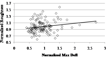
Figure 35. Graph. Normalized long-term WD-roughness versus normalized maximum deflection measured after rehabilitation in SPS-5 sites.
Similarly, the results in figure 36 suggest that maximum deflection after the pavement's rehabilitation cannot provide good qualitative information about the rutting performance predictions (p = 0.296). This observation may be contrary to what is expected. Rutting is a load-related distress, and because deflection measures the pavement's response to load applications, it seems intuitive that a positive trend might exist. However, instant deflections as measured by FWD tests were more likely to capture instantaneous elastic response of the pavement structure. Rutting is a plastic deformation more likely to occur in unbound aggregate layers and AC at warm temperatures. In rehabilitated flexible pavements, most of the permanent deformation occurred in the overlay. As temperature increases, AC behaves less like a time-dependent elastic material and more like a time-dependent plastic material. The instantaneous FWD deflections cannot be associated with the material's behavior impacting rutting performance.
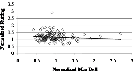
Figure 36. Graph. Normalized long-term WD-rutting versus normalized maximum deflection measured after rehabilitation in SPS-5 sections.
Contrary to expectations, the data in figure 37 indicate that no statistically significant trend was found between fatigue cracking performance and maximum deflection (p = 0.565). Conversely, the data in figure 38 suggest that higher values of transverse cracking are expected when the pavement has higher deflections (p = 0.001). The trend in figure 39 suggests that longitudinal cracking is not related to deflections measured under the center of the load on FWD tests but just marginally (p = 0.058).
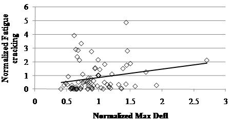
Figure 37. Graph. Normalized long-term WD-fatigue cracking versus normalized maximum deflection measured after rehabilitation in SPS-5 sections.
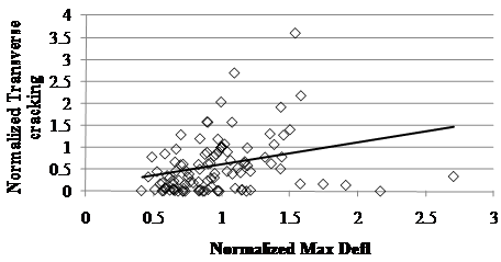
Figure 38. Graph. Normalized long-term WD-transverse cracking versus normalized maximum deflection measured after rehabilitation in SPS-5 sections.
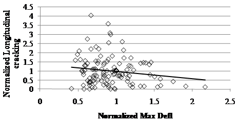
Figure 39. Graph. Normalized long-term WD-longitudinal cracking versus normalized maximum deflection measured after rehabilitation in SPS-5 sections.
Some of the distresses had clear trends with responses that agreed with the conventional wisdom and expectations of relationships between performance and response. However, none of the trends were strong enough to suggest a direct correlation between performance and response as measured by maximum deflection. These plots only suggested that deflection could be used to infer qualitative assessments of future performance of some distresses but not to quantitatively predict performance.

