Evaluation of Joint and Crack Load Transfer Final Report

Previous | Table of Contents | Next

Load Transfer Efficiency

When a traffic load is applied near a joint in a PCC pavement, both loaded and unloaded slabs deflect because a portion of the load applied to the loaded slab is transferred to the unloaded slab.  As a result, deflections and stresses in the loaded slab may be significantly less than if, instead of a joint with another slab, there was a free edge.  The magnitude of reduction in stresses and deflections by a joint compared to a free edge depends on the joint's LTE.

Traditionally, LTE at the joint is determined based on the ratio of the maximum deflection at the joint of the loaded slab and the deflection of the unloaded slab measured right across the joint from the maximum deflection.  Two equations for the deflection LTE are used most often:

(1)

and

(2)

where:

-          d_l = the maximum deflection at the joint of the loaded slab.

-          d_u = the corresponding deflection at the joint of the unloaded slab.

-          LTE and LTE* = load transfer efficiency indexes. 

If a joint exhibits a poor ability to transfer load, then the deflection of the unloaded slab is much less than the deflection at the joint of the loaded slab and both LTE indexes have values close to 0.  If joint's load transfer ability is very good, then the deflections at the both sides of the joint are equal and both indexes have values close to 100 percent.  Moreover, these two indices are related by the following equation:

(3)

Therefore, these indexes are equivalent, and if one of them is known, the other can be determined.  In this study, we will define the deflection LTE using the index from equation 1 because it is much more widely used.

The definitions of the LTE described above are based on deflections.  A joint LTE based on stress can be defined as follows:

(4)

where:

-           = the maximum stress at the joint of the loaded slab.

-           = the corresponding stress at the joint of the unloaded slab.

-          LTE = load transfer efficiency in stress.

The stress-based LTE indicates the degree of stress reduction at the joint of the loaded slab caused by the presence of the unloaded slab.  Studies have indicated that there is no one-to-one relationship between stress-based and deflection-based LTE indexes.  Because it is difficult to measure stresses in a concrete slab and stress-based LTE is much more affected by geometry of the applied load than deflection LTE, the deflection-based LTE is commonly used to measure load transfer in concrete pavements.  If deflection LTE is known, stress reduction due to load transfer for any given load configuration may be calculated using a finite element model.

Joint LTE depends on many factors, including the following:

• Joint load transfer mechanism and stiffness.
• Base/subgrade support.
• Temperature.

Load transfer between the slabs occurs through aggregate particles of the fractured surface below the saw cut at a joint, through steel dowels (if they exist), and through the base and subgrade.  LTE may vary throughout the day and year because of variation in PCC temperature.  When temperature decreases, a joint opens wider, which decreases contact between two slabs and also may decrease LTE, especially if no dowels exist.  Also, PCC slab curling may change the contact between the slab and the underlying layer and affect measured load-induced deflections.

Mechanistic Modeling of LTE

Mechanistic modeling of the load transfer mechanism is a complex problem.  Frieberg (1940) was one of the first researchers who attempted to tackle this problem.  The introduction of a finite element method for analysis of JCP (Tabatabie and Barenberg [1980]) gave a significant boost to understanding load transfer mechanisms.  However, although many comprehensive finite element models have been developed (Scarpas et al. [1994], Guo et al. [1995], Parson et al. [1997], Shoukry and William [1998], Davids et al. [1998], Khazanovich et al. [2001]), work on the development of a comprehensive, practical, and reliable model for joints of rigid pavements is far from complete. 

Ioannides and Korovesis (1990, 1992) made an important step forward in PCC joint analysis. They identified the following nondimensional parameters governing joint behavior:

Nondoweled pavements:

  (5)

Doweled pavements:

(6)

where:

-          AGG* and D^* are nondimensional stiffnesses of nondoweled and doweled joints.

-          AGG = a shear stiffness of a unit length of an aggregate interlock.

-          D = a shear stiffness of a single dowel (including dowel-PCC interaction).

-           = a PCC slab radius of relative stiffness.

-          k = subgrade k-value.

-          s = dowel spacing.

Using the finite element program ILLI-SLAB, Ioannides and Korovesis also identified a unique relationship between these parameters and LTE (see figure 1).

Figure 1. LTE versus nondimensional joint stiffness.

The following assumptions were made in derivation of these relationships:

• Prior to loading, PCC slabs are flat and in full contact with the foundation.
• A PCC joint propagates through the base layer (if present).  No load transfer occurs through the base layer.
• The subgrade is modeled as a Winkler foundation, which assumes no load transfer through the subgrade.
• The PCC joint has uniform LTE across its width. The entire load transfer in nondoweled joints occurs through aggregate interlock, whereas the entire load transfer in doweled joints occurs through dowels (no aggregate interlock).

The relationships developed by Ioannides and Korovesis form a basis for back calculation of joint aggregate interlock stiffness of nondoweled joints or dowel shear stiffness of doweled joints if their LTEs are known.  In both cases, however, the backcalculated stiffness overestimates real aggregate interlock stiffness or dowel stiffness because the entire joint stiffness is attributed to a single (although perhaps prevailing) component.  The cause of this limitation is the inability of the ILLI-SLAB model to distinguish between load transfer mechanisms.  This limitation does not cause a significant problem because the backcalculated joint stiffness provides sufficient information for accurate joint modeling in the forward analysis.  Moreover, if the addition information is available, individual components can be determined more accurately.

For example, if AGG_tot is the backcalculated stiffness of a doweled joint and D is the known dowel stiffness, then the "true" aggregate interlock factor, AGG₀, for this joint can be determined from the following relationship:

(7)

where:

-          s = dowel spacing.

In this study, Ioannides and Korovesis's relationship was further investigated and an efficient backcalculation procedure for joint stiffness determination was developed.

Joint Stiffness Backcalculation

The relationship identified by Ioannides and Korovesis was further elaborated by Crovetti (1994), Zollinger et al. (1999), and Ioannides et al. (1996).  Crovetti and Zollinger developed regression models for that relationship, whereas Ioannides and Hammons developed a neural network prediction model. 

Crovetti proposed the following relationship between nondimensional joint stiffness and LTE:

                                                           (8)

where:

-          AGG_tot = the total stiffness.

-           = the PCC slab radius of relative stiffness.

-          k = a coefficient of subgrade reaction (k-value).

Zollinger's model for this relationship has the following form:

                                                       (9)

where

-          AGG_tot = the total joint stiffness.

-           = the PCC slab radius of relative stiffness.

-          k = the subgrade k-value.

-          a = the equivalent radius of the applied load.

The neural network model developed by Ioannides and Hammons cannot be expressed as a simple equation, but rather takes the form of a computer program that relates LTE and joint stiffness, radius of relative stiffness, subgrade k-value, and load geometry.  Although this model is more accurate than the regression models, it is not publicly available and was not evaluated in this study.

To evaluate the Crovetti and Zollinger models, a factorial of 375 runs was performed to simulate FWD testing at the PCC joint.  ISLAB2000 (Khazanovich et al. [2000]) is a completely rewritten version of ILLI-SLAB that retains all the positive features of ILLI-SLAB but is more convenient to use and is free from many unnecessary limitations (including limitation on the number of nodes in a finite element model).

A finite element model developed in this study has four slabs in the longitudinal direction and three slabs in the transverse direction.  The system was assumed to be symmetrical with respect to the longitudinal axis, so only half of the system was modeled.  Because the focus of this analysis was on the deflections near the loaded joint along the centerline, a much finer finite element mesh was used along the centerline and loaded joint, as shown in figure 2.  The LTE of longitudinal joints was selected to be equal to 70 percent.  Also, due to symmetry, only half of an FWD load was applied.  The slab radius of relative stiffness was varied from 508 to

2,032 mm (80 inches), and the nondimensional transverse joint stiffness was varied from 0.1 to 278, which resulted in LTE from 8 to 99 percent.

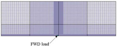
Figure 2.  Finite element model for FWD loading simulation.

Figure 3 presents comparisons of the LTEs calculated from the ISLAB2000 results and LTEs from Crovetti's and Zollinger's equations.  Although Crovetti's equation is simpler than Zollinger's, it better corresponds with ISLAB2000 LTEs.  Because the Crovetti model was adopted for use in the 2002 design procedure (National Cooperative Highway Research Program Project 1-37A) and it compares well with the finite element analysis, it was selected for use in this study.

Figure 3.  Comparison of LTE calculated from ISLAB2000 results with predictions using Crovetti's and Zollinger's models.

"True" versus "Measured" LTE

As stated above, the joint LTE is a ratio of the maximum deflection at the joint of the unloaded slab to the deflection of the loaded slab measured directly across the joint from the maximum deflection.  However, measurement of such deflections in the field may be quite cumbersome.  In the LTPP program, joint deflection testing is conducted by placing the load plate tangential to the edge of the joint.  The loaded slab joint deflections are measured under the center of the load plate (152 mm [6 inches] away from the joint).  The deflection of the unloaded slab is also measured at some distance (152 mm [6 inches]) from the joints.  This raises an issue about the possibility of error as a result of differences in deflections directly at the joint and measured deflections 152 mm (6 inches) away from the joint because of slab bending.  Some experts advocate the need to use a correction ("bending") factor to adjust the measured deflections.

To investigate this problem, the results of the 375 ISLAB2000 runs were analyzed.  The LTEs calculated from the deflections located exactly at the joints ("true" LTEs) were compared to the ratios of the deflections located 152 mm (6 inches) away from the joint ("measured" LTEs similar to the FWD procedure).  Figure 4 presents comparisons of true and measured LTEs.

Figure 4.  Comparison of true and measured LTEs.

In most cases, measured LTE is close to true LTE.  The exceptions are the cases with very low PCC slab stiffness (radius of relative stiffness is less than 750 mm (30 inches).  For those cases, measured LTE overestimates true LTE.  To address this discrepancy, the research team attempted to develop bending correction factors. 

PCC slab bending depends primarily on the radius of relative stiffness.  Since stiffer slabs require less bending correction than slabs with low radii of relative stiffness, the following functional form was proposed for the correction factor:

                                                                     (10)

where:

-          B = the bending correction factor.

-          LTE_true = the true LTE.

-          LTE_mes = the measured LTE.

-           = the radius of relative stiffness.

-          a₁ and a₂ = model parameters.

A regression analysis was performed to determine coefficients a₁ and a₂ and the following expression for the bending factor was obtained:

                                                                       (11)

R²  = 0.9998

SEE = 0.000495

where:

-           = a radius of relative stiffness in mm.

Although the correction factor has excellent statistics, its practical applicability is quite limited because the radius of relative stiffness may be unknown.  To avoid this limitation, a correction factor based on sensor deflections located on the leave slab was used to correct measured LTE.  The AREA parameter was used for this purpose.  This parameter combines the effect of several measured deflections in the basin and is defined as follows:

           (12)

where:

-          W_i = measured deflections (i = 0, n).

-          n    = number of FWD sensors minus 1.

-          r_i    = distances between the center of the load plate and sensors in mm.

The AREA parameter has been used extensively to analyze concrete pavement deflection basins since 1980.  Ioannides et al. (1989) identified the unique relationship between AREA and the radius of relative stiffness.  The AREA parameter is not truly an area, but rather has dimensions of length, since it is normalized with respect to one of the measured deflections in order to remove the effects of load magnitude.  For a given number and configuration of deflection sensors, AREA may be computed using the trapezoidal rule.  It was found that the correction factor depends on the AREA parameter and the magnitude of the measured LTE itself.  The following relationship between the true and measured LTE was proposed:

    (13)

where:

-          K₁, K₂, K₃, and K₄ = regression coefficients, depending on the sensor configuration used in AREA calculation.

Using the results from the 375 ISLAB2000 runs, the regression analysis for determining K₁, K₂, K₃, and K₄ was performed for the following sensor configurations:

• C6 sensor configuration (at 0, 305, 457, 610, 914, and 1524 mm).
• C5 sensor configuration (at 0, 305, 457, 610, and 914 mm).
• O5 sensor configuration (at 305, 457, 610, 914, and 1524 mm).
• O4 sensor configuration (at 305, 457, 610, and 914 mm).

Table 1 presents the determined coefficients along with basic statistics.

Table 1.  Regression coefficients for bending correction factors.

Test	Sensor Configuration	K1	K2	K3	K4	R2	SEE
Approach	O5	0.929710	23.61	-45.73	1171.28	0.99729	0.108298
Approach	O4	0.790073	116.74	-166.34	856.58	0.99724	0.231601
Leave	C6	0.924255	92.96	-508.52	5302.13	0.99727	0.163864
Leave	C5	0.806827	155.35	-491.51	3472.81	0.99715	0.366376
Leave	O5	0.923371	72.03	-182.53	2143.95	0.99729	0.114590
Leave	O4	0.764173	129.91	-209.29	1105.75	0.99720	0.296859

To investigate the applicability of the bending factor developed in the study, bending factors were calculated for more than 600,000 FWD basins from the LTPP database. Figures 5 and 6 present the distribution of these factors for the FWD basins from approach slab test calculated using the O5 sensor configuration and for the basins from the leave slab test calculated using the C6 sensor configuration.  In most cases, the correction was less than 4 percent.

During the bending factor testing using data from the LTPP database, it was found that significant discrepancies existed in measured LTEs for the same joints measured with a load plate placed on the approach and the leave side of the joint.  The correction factors presented above did not significantly reduce these discrepancies.  An additional investigation was conducted in an attempt to resolve this issue.

The finite element model used in the development of the correction factors did not account for differences in pavement responses as a result of the location of the loaded plate.  Also, the PCC slabs were assumed to be in full contact with the subgrade.  In reality, the application of a large number of a heavy axle loads moving in one direction may cause the formation of permanent voids under the leave side of the joint.  An assumption was made that those voids are responsible for the discrepancy between leave and approach test results.  In addition, PCC slab curling causes slabs to separate, creating temporary voids.  This effect also was analyzed in this study.

Figure 5.  Distribution of bending correction factors for approach slab testing based on O5 sensor configuration.

A factorial of 504 finite element runs with different temperature gradients through slab thickness, joint stiffness, and subgrade stiffness was performed.  In all cases, a 1.52-m (5-ft)-long permanent void occupying the entire leave slab width was modeled.  In half of the cases, the load was placed at the approach side of the joint, and in the other half it was placed at the leave side.  The load transfer values from the deflections induced by the loads placed at the approach side of the joint, LTE₁, were compared with the corresponding load transfer values calculated for the same systems but the load placed on the leave side on the joint, LTE₂.  Figure 7 presents a comparison of those LTEs.  As shown in the figure, the presence of a void significantly skewed computed LTE values.  The figure shows that LTEs computed from the leave slab test should be lower than those computed from the approach slab test.  Moreover, this effect may be much more pronounced than the effect of slab bending. 

Figure 6.  Distribution of bending correction factors for leave slab testing based on C6 sensor configuration.

Figure 7.  Comparison of LTEs predicted using ISLAB2000 for the approach slab test (LTE₁) and the leave slab test (LTE₂) for pavements with voids.

This analysis agrees with the analysis of LTPP data that discrepancies may exist between the LTEs computed from leave and approach tests; however, in the vast majority of cases analyzed, an opposite trend was observed.  As will be discussed in chapter 3, LTEs computed from the leave slab test usually were higher than LTEs computed from the approach slab test.  At this stage, no mechanistic explanation of this phenomenon was found.  More research is needed to address this issue.  Meanwhile, considering that the correction factors presented above did not change the calculated LTE values significantly, and that void/curling correction should be incorporated into this factor, a decision was made not to use the bending factor in this study.

Previous | Table of Contents | Next