U.S. Department of Transportation
Federal Highway Administration
1200 New Jersey Avenue, SE
Washington, DC 20590
202-366-4000
Federal Highway Administration Research and Technology
Coordinating, Developing, and Delivering Highway Transportation Innovations
 |
| This report is an archived publication and may contain dated technical, contact, and link information |
|
Publication Number: FHWA-RD-02-095 |
Previous | Table of Contents | Next
Statistically based construction specifications and acceptance procedures have been widely used by the highway profession for many years. These procedures typically specify an end result that can be measured in statistical terms and award payment in proportion to the extent to which the end result has been achieved. Most prescribe a variable level of payment reduction for varying amounts of deficient quality, and many now also include modest bonuses for quality that substantially exceeds the level that has been specified.
For such procedures to be considered equitable and defensible, they should not be punitive but should award payment that is at least approximately commensurate with the value received. To satisfy this requirement, it is necessary to base these procedures on quantitative (mathematical) models relating as-built construction quality to expected service life and value.
Consequently, current efforts tend to be directed at refining these procedures to become true PRS, specifications based on quality characteristics measured at the jobsite that can be related to the performance of the construction item in a specific, quantitative manner. For example, an obvious performance measure for highway pavement is service life. If, based on as-built quality levels, it is found that the pavement does not measure up to design standards, the relationship between construction characteristics and load-carrying capacity can be used to estimate the amount by which its service life will be shortened. This, in turn, can be combined with a LCC analysis to compute the expected loss in net present value, thus justifying an appropriate amount of payment reduction.
Obviously, a prerequisite for such a process is to first develop the mathematical models necessary to predict from quality characteristics measured at the jobsite what the expected performance of the construction item will be. In the case of pavement, the design procedure itself provides some of the necessary relationships. If the pavement is constructed with insufficient thickness, for example, it is a simple matter to work backwards through the design procedure to determine the reduced number of loads it will be capable of sustaining and, from that, its expected life can be predicted. For other characteristics, however, no such convenient relationships may exist and, in these cases, it is necessary to develop a method to obtain the required relationships from existing knowledge or data.
Although it is possible to obtain a mathematical model by performing a least-squares fit with a standard regression program, using either a linear equation or various curvilinear forms, it is often possible to obtain a better model by first using engineering knowledge to determine the most appropriate mathematical form. In many cases, using known boundary conditions to reason out the general shape of the mathematical relationship will provide a much improved model that is more likely to be accurate throughout its range, not just in the region in which most of the data are concentrated.
This appendix presents a straightforward and practical procedure by which any agency can make use of empirical performance data to develop quantitative models for expected life and value for multiple quality characteristics, thus forming the basis for rational and defensible payment adjustment schedules.
Although efforts are under way to create extremely sophisticated computerized procedures to develop performance relationships and appropriate payment schedules, the successful completion and validation of these procedures is still some time away. Even when completed, the data requirements and level of complexity of these procedures may deter their widespread use by practitioners seeking more practical methods that are easier to understand and to apply. Therefore, there is need for an alternative approach for those agencies that choose to develop their own procedures in their own way tailored to their own specific circumstances. Perhaps more importantly, this alternative method needs to be sufficiently straightforward and scientifically sound so that agency engineers can not only understand it and use it with confidence, but also can modify it when necessary and be able to present it convincingly to the contractors whose work it will govern. Without this degree of familiarity and understanding, it may not be easy to implement the new procedures in the face of the typical opposition from the construction industry, nor to explain or defend the results should they be challenged.
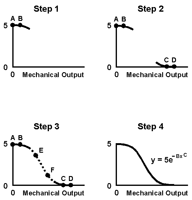
Suppose it were desired to develop a model for PSI based on the output of some measuring device that is either pushed or driven down the road. PSI is defined on a scale of 0.0 - 5.0 in which 5.0 represents perfect smoothness and 0.0 indicates a pavement that is virtually impassible. The 0.0 - 5.0 scale was initially developed for use by a team of raters to evaluate pavements of varying degrees of roughness but, to be useful as a practical evaluation tool, it is necessary to relate it to the output of some standardized mechanical measuring device.
To determine an appropriate mathematical form for this relationship, first consider the situation illustrated by point "A" in step 1 of figure 68. If a highly sensitive measuring device produces no output whatsoever (i.e., zero on the horizontal-axis), then by definition that corresponds to a PSI value of 5.0 on the vertical-axis (i.e., perfect smoothness). Next, consider point "B" at which the measuring device produces a very small reading, but the level of roughness is so slight that it is undetectable by a panel of raters. In this case, the pavement would still be rated at 5.0, even though there is a very small output from the measuring device. However, as the test pavements become rougher, both the measuring device and the panel will begin to record readings below 5.0. What this indicates is that the upper portion of the model very likely starts out horizontally from the vertical-axis at and then begins to bend downward, as indicated by the curved line through points "A" and "B" in figure 68.
|
|
Figure 68. Conceptual Steps to Develop a Performance Model for Pavement Smoothness
Next, consider the lower end of the curve shown in step 2 of figure 68. It would be possible to construct a hypothetical pavement that is so rough that the rating team would consider it impassible and rate it a zero, indicated by point "C." However, it would also be possible to construct a still rougher pavement as measured by the testing device, indicated by point "D," and this pavement would also be rated a zero because that is the minimum possible rating. What this indicates is that the curve must also be horizontal at its lower extremity, and thus comes in asymptotically to the horizontal-axis.
These two boundary conditions make it possible to narrow the range of choices for the appropriate mathematical model to an equation that produces a sigmoidal ("S") shape as shown in step 3 of figure 68. Then, if there are sufficient data in the middle region, or if one or two additional points can be identified, such as points "E" and "F" in step 3, the model can be reasonably well specified.
A convenient mathematical form to model this curve is the exponential expression given by equation 106 and shown in step 4 of figure 68. For a perfectly smooth pavement, y = 5 at x = 0, so the first coefficient is predetermined to be A = 5. The two "known" points "E" and "F" provide sufficient information to write two simultaneous equations that can be solved to obtain the remaining two coefficients in equation 106.
| |
There are two reasons why equation 106 does a good job of modeling performance relationships. The first is that it properly takes boundary conditions into account and will not return unrealistic values in the extreme regions for which data may not have been available. The second is that, since there are three unknown coefficients (A, B, and C) to be determined, this permits the model to be made to pass through three convenient known points, such as points "A," "E," and "F" in figure 68. Therefore, provided the level of performance can be estimated at three points, the entire model can be specified reasonably accurately. For a single-parameter model such as equation 106, three logical determining points would be the maximum (point "A" in figure 68), the AQL, and the RQL.
To develop a general model, it will be desirable to replace the independent variable, x, in equation 106 with a suitable statistical quality measure. Of the various measures that might be chosen, probably the most frequently used for highway construction are PWL, or its complement, the PD. These two measures, which are functionally equivalent, are intuitively appealing because they account for both mean level and variability in a single statistic.
It can be observed that the model form given by equation 106 is especially well suited when zero is the most favorable level of x, as is the case when PD is substituted for x as the quality measure. When x = 0 is not the most favorable level, as is the case with PWL, a somewhat more complex equation form will be necessary. However, if it is desired to develop the model in terms of PWL, it will be found that it is better to first develop it in terms of PD, and then substitute (100 - PWL) for PD at the last step. Because the measure PD is the more natural fit for this equation form, it is used in the developments that follow.
Using equation 106 as a guide, the logical form for a multiple-parameter model is given by equation 107:
|
(107) |
It is shown later, however, that a very serviceable model can be obtained without the need for the added complexity of the individual "C" exponents in equation 107, so they are omitted in the equation to be developed. Since PD is the more natural fit for the single-parameter model given by equation 106, it is selected as the independent variable for use with the multiple-parameter model. Finally, since it is desired to obtain an expression for expected service life as a function of as-built quality, the variable EXPLIF is substituted for y as the dependent variable, producing equation 108, in which e is the base of natural logarithms. (The final proof of this model is an extensive series of tests to demonstrate that it reliably produces results that are consistent with field experience.)
|
(108) |
To solve for the unknown coefficients in equation 108, it is first necessary to take logarithms of both sides, producing equation 109:
| |
(109) |
At this point, it is convenient to observe that the term ln(A) in equation 109 can be regarded as B0, the constant term of the multiple-parameter expression. After a set of simultaneous equations has been solved to obtain the "B" coefficients, B0 can be used to determine coefficient "A" using equation 110.
|
(110) |
To summarize up to this point, equations 106 through 110 describe the mathematical basis for a practical multiple-parameter model. The next step is to outline the data requirements for this model.
If the method is to be valid, it must be based on realistic data, and if it is to be practical, the required data must be readily obtainable. Table 52 is a generic data matrix that must be completed to apply this method.
|
PD1 |
PD2 |
PD3 |
® |
PDk |
EXPLIF |
|---|---|---|---|---|---|
|
AQL(1) | AQL(2) | AQL(3) | ® | AQL(k) | DESLIF |
| POOR(1) |
AQL(2) | AQL(3) | ® | AQL(k) | LIFE(1) |
|
AQL(1) | POOR(2) | AQL(3) | ® | AQL(k) | LIFE(2) |
|
AQL(1) | AQL(2) | POOR(3) | ® | AQL(k) | LIFE(3) |
|
¯ | ¯ | ¯ | ® | ¯ | ¯ |
|
AQL(1) | AQL(2) | AQL(3) | ® | POOR(k) | LIFE(n) |
PDi = percent defective for each of the k quality characteristics.
EXPLIF = expected life in years.
DESLIF = design life in years.
AQL(i) = acceptable quality level, in PD, for each of the k quality
characteristics.
POOR(i) = poor quality level, in PD, for each of the k quality characteristics.
LIFE(m) = expected life in years for n selected combinations of PD levels.
It can be seen from the first row in table 52 that, when all quality characteristics are at their respective AQL values, the expected life is equal to the design life. For the remainder of the rows in this table, each characteristic in turn is set at some specified poor level of quality (which might appropriately be the RQL) while all the others are held constant at the AQL. It is believed that this provides the most convenient arrangement of performance data that an agency might be expected to have, or could obtain relatively easily. The values to be entered in the table might be developed as the collective opinion of experienced pavement engineers, or they might be obtained more formally through a multiple regression analysis of actual field data. In some cases, the agency's current pavement design method may be able to provide some of this information.
The next section demonstrates how easy it is to convert the data in this matrix to a performance model of the general form given by equation 108.
For demonstration purposes, consider a specification for HMAC pavement for which the agency wishes to control three quality characteristics: in-place air voids, thickness, and smoothness. A typical value for the AQL is PD = 10, while RQL values tend to vary more widely, depending on what level of quality an agency believes justifies potential removal and replacement. For this example, the values listed in table 53 have been selected.
|
Quality Characteristic |
PD (AQL) |
PD (RQL) |
|---|---|---|
|
Air Voids | 10 |
65 |
|
Thickness | 10 |
75 |
|
Smoothness | 10 |
85 |
The values in table 53, plus the design life for a typical overlay of 10 years, are entered into the general matrix of table 52, producing table 54:
|
PDVOIDS |
PDTHICK |
PDSMOOTH |
EXPLIF, in years |
|---|---|---|---|
10 (AQL) | 10 (AQL) | 10 (AQL) | 10 (DESLIF) |
65 (RQL) | 10 (AQL) | 10 (AQL) | LIFE (poor voids) |
10 (AQL) | 75 (RQL) | 10 (AQL) | LIFE (poor thickness) |
10 (AQL) | 10 (AQL) | 85 (RQL) | LIFE (poor smoothness) |
By now, the ease of applying this method should be apparent. The only additional pieces of information required are realistic estimates of expected service life for the three conditions specified in the last three rows of table 54, using any of the methods suggested in the previous section. For purposes of this example, assume that the agency has selected the respective individual RQL values in the belief that they will produce a loss of service life of about 50 percent, producing an expected life of 5 years for each of these rows. The final performance matrix is presented in table 55.
|
PDVOIDS |
PDTHICK |
PDSMOOTH |
EXPLIF, in years |
|---|---|---|---|
|
10 | 10 |
10 |
10 |
|
65 | 10 |
10 |
5 |
| 10 |
75 |
10 |
5 |
| 10 |
10 |
85 |
5 |
All that remains now is to substitute the information from the final performance matrix in table 55 into equation 109 to produce the necessary set of simultaneous equations. These are presented as equations 111 through 114:
2.302585 = B0 - 10B1 - 10B2 - 10B3 (111)
1.609440 = B0 - 65B1 - 10B2 - 10B3 (112)
1.609440 = B0 - 10B1 - 75B2 - 10B3 (113)
1.609440 = B0 - 10B1 - 10B2 - 85B3 (114)
These equations could be solved by hand, but there are any number of computer packages that will do this, producing the following results:
B0 = 2.627669
B1 = 0.012603
B2 = 0.010664
B3 = 0.009242
Then, using equation 110,
![]()
All the necessary constant terms have now been determined and the complete performance model can be written as equation 115.
The first test of equation 115 is to check that it returns precisely the values
from table 55 that were used to derive it. These results are presented in
table 56.
Values Entered into Equation 115 |
EXPLIF Returned, in years |
||
|---|---|---|---|
PDVOIDS |
PDTHICK |
PDSMOOTH |
|
10 |
10 |
10 |
10.0 |
65 |
10 |
10 |
5.0 |
10 |
75 |
10 |
5.0 |
10 |
10 |
85 |
5.0 |
It is seen from table 56 that the model survives the first test because it returns exactly the appropriate values. A second test is to check the extremes, an area in which many models break down. The extremes in this case occur when all three PD values are either 0 or 100. These results are presented in table 57.
| Values Entered into Equation 115 |
EXPLIF Returned, in years |
||
|---|---|---|---|
PDVOIDS |
PDTHICK |
PDSMOOTH |
|
0 |
0 |
0 |
13.8 |
100 |
100 |
100 |
0.5 |
Here again, the values returned by the performance model in equation 115 appear to be appropriate. It is not unreasonable to expect that a few exceptionally well constructed overlays may last 14 years, and in some cases, even longer. Therefore, the prediction by this model that the highest possible quality level would lead to an expected life of nearly 14 years seems reasonable. At the other extreme, the failure of a pavement during the first year is certainly rare, but it has occurred, so the prediction that the worst possible quality level (100 percent defective in all characteristics) could produce such an early failure may well be realistic. At this stage, the model is judged to be believable, but several additional tests are required.
The predicted life for a wide variety of combinations of individual quality levels of the three characteristics is presented in table 58. The first group of tests provides a sense of how expected life decreases as the three quality measures decline together. The second set of tests in this table illustrates how extra quality in some characteristics can offset deficient quality in other characteristics, all producing the design life of 10 years. This is an inherent feature in most design methods, and is believed to be an appropriate feature in any model of multiple characteristics. The only concern would be if extremely poor quality (100 percent defective) in one characteristic could be masked by superior quality in other characteristics, and the third group of tests indicates this is not the case.
| Values Entered into Equation 115 |
EXPLIF Returned, in years |
||
|---|---|---|---|
PDVOIDS |
PDTHICK |
PDSMOOTH |
|
0 |
0 |
0 |
13.8 |
10 |
10 |
10 |
10.0 |
25 |
25 |
25 |
6.1 |
50 |
50 |
50 |
2.7 |
75 |
75 |
75 |
1.2 |
100 |
100 |
100 |
0.8 |
17 |
10 |
0 |
10.0 |
0 |
21 |
10 |
10.0 |
0 |
10 |
23 |
10.0 |
25 |
0 |
0 |
10.1 |
0 |
30 |
0 |
10.0 |
0 |
0 |
35 |
10.0 |
0 |
0 |
100 |
5.5 |
0 |
100 |
0 |
4.7 |
100 |
0 |
0 |
3.9 |
0 |
0 |
50 |
8.7 |
0 |
50 |
0 |
8.1 |
50 |
0 |
0 |
7.3 |
The final group of tests in table 58 is included to investigate the extent to which moderately poor quality (50 percent defective) could be offset by excellent quality in the other two characteristics. These three cases are examined individually, beginning with the smoothness case in the third row from the bottom in table 58. Using an upper specification limit of an IRI of 1.18 m/km and a typical standard deviation based on one agency's data of about σ = 0.24 m/km, the largest IRI value in a section of pavement having PD = 50 would be about three standard deviations above the limit, or about 1.90 m/km. According to recent literature on pavement profiling, (26) even new pavements may range up to about IRI = 3.16 m/km, so a newly constructed pavement having PD = 50 should have a considerable amount of service life remaining. Therefore, the expected life of 8.7 years predicted by equation 115 in table 58 appears to be reasonable.
In the next to last row of table 58, it is seen that a thickness quality level of PD = 50, combined with PD = 0 in the other two characteristics, produces an expected life of 8.1 years. To check this case, the AASHTO Design Procedure for Flexible Pavement is used. (31) Using a typical 100-mm overlay and nominal values for the various other variables (layer coefficient, resilient modulus, terminal serviceability, thickness standard deviation, etc.), it was calculated that a decrease in thickness quality from the AQL of PD = 10 to a moderately defective level of PD = 50 would result in a loss of load-carrying capacity of about 40 percent. Based on the design life of 10 years, the resultant life expectancy would then be about 6 years, somewhat lower than the value of 8.1 years in table 58. However, this calculation with the AASHTO design procedure assumes that other variables that are not included in the design procedure are at nominal satisfactory levels, whereas the example in table 58 has both air voids and smoothness at the best possible quality level of PD = 0. Therefore, it is logical to assume that this might raise the overall performance somewhat, and the predicted life of 8.1 years may be reasonable after all.
To perform a rough check on the last row of table 58, published information on the effects of HMAC compaction is used. It has been reported that the expected life of HMAC pavement decreases by approximately 10 percent for each 1.0 percent increase in the level of air voids above 7.0 percent. (33) Based on typical data from one agency, a decrease in quality from the acceptable level of PD = 10 to a defective level of PD = 50 requires a shift in average level of about 2.0 to 3.0 percent, so 2.5 percent is used here. Using the relationship cited above, this would correspond to a loss of life of 25 percent, or an expected life of about 7.5 years. This might appear to be in close agreement with the value of 7.3 years in table 58, but, as in the previous calculation, this does not account for the potentially beneficial effect of excellent quality in the other two variables, so the true value may be higher. However, since the information used to perform this check is only approximate, this may still be a reasonably close check for practical purposes.
Table 58 also provides the opportunity to observe the effects of changes in the individual quality characteristics. Going back to the values in the performance matrix in table 55, it can be seen that, based on the data used in this example, air voids has the greatest influence because it requires the smallest amount of percent defective (PD = 65) to reduce the expected life to 5 years, while smoothness has the least effect because it requires the greatest amount of percent defective (PD = 85) to produce the same effect. The second, third, and fourth groups of data in table 58 all demonstrate the consistency of the relative importance of these three variables. If a different combination of relative importance were desired, then different values would be used in the final performance matrix in table 55.
In summary, all of the checks of the model given by equation 115 have shown it to be both reasonable and consistent. More importantly, this method will reliably produce models that will accurately and consistently reflect the information entered into the performance matrices from which they are derived.
The next step of this process is to determine the economic impact of the estimate of expected life obtained with the performance model. A practical repair strategy for HMAC pavement is particularly well suited for LCC analysis that can be used to properly discount future expenses. For at least some agencies, it is not normal practice to perform special maintenance actions just to restore the design life of a HMAC pavement that was constructed with some sort of quality deficiency. (An obvious exception would be a safety issue.) Instead, the condition of the pavement is monitored and, when premature failure begins to occur, the pavement is scheduled for an overlay. The availability of a performance model to predict when this premature failure will occur is obviously a critical component of an acceptance scheme designed to award payment in proportion to expected performance.
On the assumption that an estimate of expected life is available, and that it is justifiable to assign a payment reduction equivalent to the loss in net present value resulting from premature failure as the result of insufficient quality of items under the contractor's control, equation 116 is derived in appendix I:
(116) |
where: PAYADJ = appropriate payment adjustment for new pavement or overlay (same units as C).
C = present total cost of resurfacing. (typical value = $23.92/m2).
D = design life of pavement or initial overlay (typically 20 years for new pavement, 10 years for overlay).
E = expected life of pavement or overlay (variable).
O = expected life of successive overlays (typically 10 years).
R = (1 + INF) / (1 + INT).
INF = long-term annual inflation rate in decimal form (typically 0.04).
INT = long-term annual interest rate in decimal form (typically 0.08).
Table 59 has been constructed to show that equation 116 justifies relatively large payment adjustments that reflect real costs (or benefits) to the agency when the actual quality differs substantially from the design quality. Many possible combinations of quality levels are included, arranged in descending order from best to worst. Note that, although appropriate payment levels have been computed for all cases, many agencies would choose to have an RQL provision supersede the payment schedule for extremely low values of expected life, providing the option to require removal and replacement at the time of construction.
It is believed that few, if any, agencies use payment adjustments as large as those computed in table 59, possibly because they have lacked a firm basis to justify values this large. However, another explanation could be that it often is possible to get the desired response from the construction industry without using the maximum amount of payment adjustment that would be economically justifiable. In other words, the level of payment adjustment only needs to be large enough to provide a strong incentive to the contractor to produce good quality initially. The
Individual Quality Levels |
Expected Life, in years |
Payment Adjustment1, in $/Lane Kilometer |
||
|---|---|---|---|---|
PDVOIDS |
PDTHICK |
PDSMOOTH |
||
0 |
0 |
0 |
13.8 |
+25,484 |
5 |
0 |
5 |
12.4 |
+16,517 |
5 |
5 |
5 |
11.8 |
+12,527 |
10 |
10 |
10 |
10.0 |
0 |
0 |
0 |
45 |
9.1 |
-6,590 |
0 |
45 |
0 |
8.6 |
-10,349 |
45 |
0 |
0 |
7.9 |
-15,732 |
25 |
15 |
30 |
6.5 |
-26,935 |
40 |
15 |
30 |
5.4 |
-36,162 |
40 |
30 |
30 |
4.6 |
-43,117 |
40 |
30 |
55 |
3.6 |
-52,112 |
65 |
30 |
55 |
2.7 |
-60,502 |
65 |
75 |
55 |
1.6 |
-71,152 |
90 |
90 |
90 |
0.7 |
-80,202 |
1 Computed using equation 116 and associated constants.
significance of this is that, if payment schedules substantially less severe than those that would be justifiable are typically used, then the performance models upon which the payment schedules are based do not have to be known with great precision. Therefore, models developed by the method outlined in this appendix are believed to be more than adequate for their intended use.
The final step of this process is to convert the information in table 59 into a workable payment equation. The easiest way to do this is to first plot the appropriate payment adjustment from table 59 versus expected life, as shown in figure 69. This relationship plots so nearly as a straight line that it could be approximated with a simple linear payment equation, if desired. However, in addition to the large payment reductions justified by the LCC analysis, this would also produce bonus payment factors that would be quite large. While bonus provisions are now widely used by agencies throughout the United States, top management has usually insisted that they be limited at some reasonable level, partly due to budget limitations and partly due to the possibility that a pavement might fail to achieve the expected extended life due to some condition not accounted for by the acceptance procedure.
A very practical way to address this issue, which has been used by one agency and has been well received by the construction industry in that State, is to use a compound payment equation as shown in figure 69. This has the twofold benefit of keeping the bonus provision within sensible limits and also dealing less harshly with a contractor whose work deviates only marginally from the desired quality level. It does, however, retain the safeguard of assessing large payment reductions for work that departs substantially from the desired level.
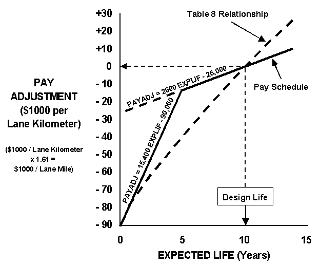
Figure 69. Payment Schedule Developed from Table 59
For this example, assume that management has decided that the maximum bonus to be paid will be no larger than $10,000 per lane kilometer. Since the maximum value of expected life returned by the performance model given by equation 115 is 13.8 years, and the design life used in this example for a typical overlay is 10 years, the upper portion of the payment equation must pass through the two points, x = 13.8, y = 10,000 and x = 10, y = 0. The slope, therefore, is computed as (10,000 - 0)/(13.8 - 10) = 2632, so 2600 will be used. The intercept is found by computing
0 - 2600(10 - 0) = -26,000 $/lane kilometer. The payment equation for this portion of the payment schedule is given by equation 117 and is also shown in figure 69.
| PAYADJ = 2600 (EXPLIF) - 26,000 | (117) |
where: PAYADJ = payment adjustment in units of $/lane kilometer.
EXPLIF = expected life (years) obtained from equation 115.
For the lower part of the compound payment equation, it must be decided where the breakpoint is to be placed, and 5.0 years will be used for this example. The graph in figure 69 is used to determine -90,000 to be a suitable intercept. Then, since this payment equation must intersect the upper payment equation at x = 5, equation 117 is used to compute the ordinate at that point to be y = 2600(5) - 26,000 = -13,000. The slope is then obtained by computing (90,000 - 13,000)/(5 - 0) = 15,400, and the resulting payment equation is given by equation 118 and also shown in figure 69, in which all terms are as previously defined.
| PAYADJ = 15,400 (EXPLIF) - 90,000 | (118) |
It should be noted that equations 117 and 118 represent just one of many suitable payment schedules that could be developed from the information in table 59 and the plot in figure 69. Either payment equation could be slightly steeper or shallower, provided they intersect at the breakpoint of EXPLIF = 5 years used in this example. The choice of breakpoint is purely a practical one, also, and a different breakpoint could have been used, if desired.
Finally, it is likely that most agencies would want to define an RQL in terms of expected life below which the agency has the option to require removal and replacement of the pavement at the contractor's expense. One possibility, suggested by the graph in figure 69, would be to define the RQL as a pavement whose expected life is less than 5.0 years. In this case, the lower portion of the payment schedule given by equation 118 would only come into play if the agency chose to waive the RQL provision.
Yet another possibility that may be appropriate is for the agency to specify that retests be performed to confirm the RQL condition before imposing the requirement to remove and replace the pavement. In this case, the upper payment equation would apply if the agency elected not to retest, and the lower payment equation would apply if the agency performed the retests, confirmed the RQL condition, but chose to waive the option to require removal and replacement.
A procedure has been presented that enables highway engineers with only a basic knowledge of engineering mathematics to use empirical construction data to develop realistic models for multiple quality characteristics, and to use those models to establish practical, effective, and defensible payment equations for QA specifications. The method is specifically designed to be easy to apply, and to avoid some of the problems to which other modeling methods may be prone, such as excessive complexity and the tendency to return unrealistic values when very large or very small input values must be used. A complete example was included for which performance data for three characteristics of HMAC pavement-in-place air voids, thickness, and smoothness-were used to develop a model for expected life. A simple LCC analysis was then applied to determine an appropriate payment schedule. The fact that this approach operates in two stages-first estimating expected life and then determining an appropriate payment adjustment-is believed to be desirable in that it will provide the type of information necessary to develop more accurate models in the future. Although the need to handle more than three quality characteristics at a time may be rare, the modeling method is sufficiently straightforward that additional characteristics can easily be accommodated, if necessary. Earlier versions of this approach have been used by one agency for several years, and their success has been reflected both in the quality achieved and the generally good working relationship the agency continues to have with the construction industry in the State.