U.S. Department of Transportation
Federal Highway Administration
1200 New Jersey Avenue, SE
Washington, DC 20590
202-366-4000
Federal Highway Administration Research and Technology
Coordinating, Developing, and Delivering Highway Transportation Innovations
 |
| This report is an archived publication and may contain dated technical, contact, and link information |
|
Publication Number: FHWA-HRT-04-046 Date: October 2004 |
Previous | Table of Contents | Next
As noted in chapter 5, the PWL and AAD quality measures were selected for additional analyses, while the CI was eliminated from further study. The use of each of these measures is based on the assumption that the population that is being sampled is normally distributed. To determine how robust these measures are, computer simulation was used to evaluate how they performed when the sampled population was not normally distributed.
The most likely departures from normality would be skewed or bimodal distribution of data. Computer simulation programs were developed to evaluate the performance of the PWL and AAD estimators under each of these situations. The following sections of this chapter present the results for analyses conducted using these simulation programs.
Skewed distributions usually occur because of some physical boundary that comes into play for a particular characteristic. For example, the percent passing a sieve for gradation analysis cannot exceed 100 percent. Thus, if the average percent passing is near 100, say 95 percent, it is possible to have greater spread on the low side of the average than on the high side. Another barrier might be pavement thickness, which cannot be less than zero. These cases are similar in concept to the discussions in chapter 5 regarding why the distributions of sample AAD and CI values have skewed distributions. The following sections present the results of computer simulation analyses on the effects of skewness on the estimates for PWL and AAD.
Two computer simulation programs were developed to investigate the performance of the PWL estimating procedures when working with a skewed distribution. One program is for use with one-sided specifications, while the other is for two-sided specifications. Skewness is measured by a skewness coefficient that equals zero for a symmetrical distribution and which increases as the distribution becomes more highly skewed. The skewness for a data set can be calculated from the following equation:
 (6)
(6)
A skewness value of zero indicates that the distribution of data is symmetrical. The skewness can be either positive or negative. Positive skewness indicates a distribution with the long tail to the right, while negative skewness indicates that the long tail is to the left. Table 16 illustrates distributions with various levels of skewness.
Table 16. Distributions with various levels of skewness.
| Skewness Coefficient | Positive | Negative |
|---|---|---|
| 0.0 |  |
|
| 0.5 |  |
 |
| 1.0 |  |
 |
| 1.5 |  |
 |
| 2.0 |  |
 |
| 3.0 |  |
 |
Both of the programs begin with a data set that is normally distributed. An exponent, entered by the user, is then used to transform these data to the skewed distribution desired.
One-Sided Limit: Computer simulation was used to evaluate the PWL estimates for populations with skewness coefficients of 0, +0.5, -0.5, +1.0, -1.0, +1.5, -1.5, +2.0, -2.0, +2.5, -2.5, +3.0, and -3.0. Sample sizes = 3, 5, and 10 were used to estimate the PWL values for populations with each of these skewness coefficients. In each analysis, 10,000 samples of the appropriate size were generated from a population with one of the skewness coefficients. The average bias and variability were then determined for the 10,000 PWL estimates. The results of these simulations are shown in tables 17 through 19 for sample sizes = 3, 5, and 10, respectively.
For efficiency, the simulation program calculates the bias and standard deviation only for positive skewness coefficients, it then reverses these numbers and their signs to obtain the values for negative skewness (i.e., the bias for 90 PWL with positive skewness is equal to -1 times the bias for 10 PWL with negative skewness). This is apparent in tables 17 through 19.
Figures 19 through 21 graphically present the bias results from tables 17 through 19, respectively. These figures plot the bias versus the actual PWL value for each of the levels of skewness. Figures 19 through 21 present the results for samples sizes = 3, 5, and 10, respectively.
The trends are obvious. The greater the skewness, the greater the bias in the PWL estimate. This is logical since the distributions deviate more from normality (on which the PWL calculation is based) as the skewness increases. The values for positive and negative skewness are mirror images of each other.
Table 20 presents a portion of the bias results from tables 17 through 19. The results are sorted by the amount of skewness, with skewness coefficients of 1.0, 2.0, and 3.0 included. Figure 22 presents the bias results from table 20 plotted by sample sizes = 3, 5, and 10 for equal levels of skewness. It should be noted that for negative skewness, the magnitude of the biases would be the same; however, the plots would be flipped vertically about the bias value of zero.
Interestingly, figure 22 shows that the larger the sample size, the greater the bias of the estimate. This probably stems from the fact that the larger sample does a better job of estimating PWL for the assumed symmetrical normal distribution. This leads to a greater bias since the population is actually a skewed distribution rather than a symmetrical normal distribution.
Table 17. Bias in estimating PWL for various skewness coefficients and one-sided limits (3 tests per lot and 10,000 simulated lots).
| PWL | +0.0 | +0.5 | +1.0 | +1.5 | +2.0 | +2.5 | +3.0 |
|---|---|---|---|---|---|---|---|
| 99 | +0.04 | -0.35 | -1.26 | -2.33 | -3.57 | -4.96 | -6.57 |
| 95 | -0.04 | -0.60 | -1.27 | -2.35 | -3.14 | -4.31 | -5.43 |
| 90 | -0.01 | -0.33 | -1.04 | -1.63 | -2.11 | -2.88 | -3.65 |
| 80 | +0.35 | +0.23 | +0.25 | -0.23 | -0.41 | -0.45 | -0.53 |
| 70 | +0.64 | +0.72 | +0.77 | +1.42 | +0.81 | +1.41 | +1.39 |
| 60 | -0.12 | +0.11 | +1.21 | +1.69 | +2.04 | +2.53 | +2.82 |
| 50 | -0.35 | +0.61 | +1.61 | +2.13 | +2.95 | +3.20 | +3.67 |
| 40 | +0.14 | +0.83 | +0.81 | +2.03 | +2.94 | +3.13 | +3.76 |
| 30 | -0.10 | +0.61 | +1.11 | +1.63 | +2.07 | +2.22 | +2.95 |
| 20 | -0.31 | +0.07 | +0.54 | +0.90 | +1.77 | +1.43 | +1.87 |
| 10 | +0.11 | -0.19 | -0.10 | -0.16 | +0.33 | +0.51 | +0.23 |
| 5 | +0.02 | -0.21 | -0.05 | -0.27 | -0.33 | -0.17 | -0.10 |
| 1 | +0.06 | -0.12 | -0.19 | -0.22 | -0.21 | -0.20 | -0.22 |
| PWL | -0.0 | -0.5 | -1.0 | -1.5 | -2.0 | -2.5 | -3.0 |
|---|---|---|---|---|---|---|---|
| 99 | -0.06 | +0.12 | +0.19 | +0.22 | +0.21 | +0.20 | +0.22 |
| 95 | -0.02 | +0.21 | +0.05 | +0.27 | +0.33 | +0.17 | +0.10 |
| 90 | -0.11 | +0.19 | +0.10 | +0.16 | -0.33 | -0.51 | -0.23 |
| 80 | +0.31 | -0.07 | -0.54 | -0.90 | -1.77 | -1.43 | -1.87 |
| 70 | +0.10 | -0.61 | -1.11 | -1.63 | -2.07 | -2.22 | -2.95 |
| 60 | -0.14 | -0.83 | -0.81 | -2.03 | -2.94 | -3.13 | -3.76 |
| 50 | +0.35 | -0.61 | -1.61 | -2.13 | -2.95 | -3.20 | -3.67 |
| 40 | +0.12 | -0.11 | -1.21 | -1.69 | -2.04 | -2.53 | -2.82 |
| 30 | -0.64 | -0.72 | -0.77 | -1.42 | -0.81 | -1.41 | -1.39 |
| 20 | -0.35 | -0.23 | -0.25 | +0.23 | +0.41 | +0.45 | +0.53 |
| 10 | +0.01 | +0.33 | +1.04 | +1.63 | +2.11 | +2.88 | +3.65 |
| 5 | +0.04 | +0.60 | +1.27 | +2.35 | +3.14 | +4.31 | +5.43 |
| 1 | -0.04 | +0.35 | +1.26 | +2.33 | +3.57 | +4.96 | +6.57 |
Note: The values shown in the table are calculated by subtracting the actual population
PWL value from the average of the 10,000 estimated lot PWL values.
Table 18. Bias in estimating PWL for various skewness coefficientsand one-sided limits (5 tests per lot and 10,000 simulated lots).
| PWL | +0.0 | +0.5 | +1.0 | +1.5 | +2.0 | +2.5 | +3.0 |
|---|---|---|---|---|---|---|---|
| 99 | +0.03 | -0.78 | -2.27 | -4.31 | -6.27 | -8.22 | -9.96 |
| 95 | -0.20 | -0.97 | -2.34 | -4.05 | -5.32 | -6.89 | -8.26 |
| 90 | -0.03 | -0.56 | -1.65 | -2.54 | -3.72 | -4.76 | -5.68 |
| 80 | -0.20 | +0.22 | +0.15 | +0.14 | +0.01 | -0.40 | -0.65 |
| 70 | -0.46 | +1.04 | +1.79 | +2.37 | +2.74 | +3.04 | +3.14 |
| 60 | -0.19 | +1.24 | +2.54 | +3.58 | +4.90 | +5.36 | +5.47 |
| 50 | -0.02 | +1.15 | +3.12 | +4.42 | +5.54 | +6.50 | +7.17 |
| 40 | -0.08 | +1.44 | +3.24 | +4.68 | +5.42 | +6.36 | +7.30 |
| 30 | -0.03 | +1.17 | +2.13 | +3.02 | +4.21 | +5.29 | +6.13 |
| 20 | +0.39 | +0.16 | +0.97 | +1.58 | +2.26 | +2.82 | +3.81 |
| 10 | -0.13 | -0.44 | -0.47 | -0.12 | +0.35 | +0.43 | +0.80 |
| 5 | -0.04 | -0.77 | -0.86 | -0.70 | -0.77 | -0.65 | -0.57 |
| 1 | 0.00 | -0.30 | -0.40 | -0.47 | -0.45 | -0.46 | -0.36 |
| PWL | -0.0 | -0.5 | -1.0 | -1.5 | -2.0 | -2.5 | -3.0 |
|---|---|---|---|---|---|---|---|
| 99 | 0.00 | +0.30 | +0.40 | +0.47 | +0.45 | +0.46 | +0.36 |
| 95 | +0.04 | +0.77 | +0.86 | +0.70 | +0.77 | +0.65 | +0.57 |
| 90 | +0.13 | +0.44 | +0.47 | +0.12 | -0.35 | -0.43 | -0.80 |
| 80 | -0.39 | -0.16 | -0.97 | -1.58 | -2.26 | -2.82 | -3.81 |
| 70 | +0.03 | -1.17 | -2.13 | -3.02 | -4.21 | -5.29 | -6.13 |
| 60 | +0.08 | -1.44 | -3.24 | -4.68 | -5.42 | -6.36 | -7.30 |
| 50 | +0.02 | -1.15 | -3.12 | -4.42 | -5.54 | -6.50 | -7.17 |
| 40 | +0.19 | -1.24 | -2.54 | -3.58 | -4.90 | -5.36 | -5.47 |
| 30 | +0.46 | -1.04 | -1.79 | -2.37 | -2.74 | -3.04 | -3.14 |
| 20 | +0.20 | -0.22 | -0.15 | -0.14 | -0.01 | +0.40 | +0.65 |
| 10 | +0.03 | +0.56 | +1.65 | +2.54 | +3.72 | +4.76 | +5.68 |
| 5 | +0.20 | +0.97 | +2.34 | +4.05 | +5.32 | +6.89 | +8.26 |
| 1 | -0.03 | +0.78 | +2.27 | +4.31 | +6.27 | +8.22 | +9.96 |
Note: The values shown in the table are calculated by subtracting the actual population
PWL value from the average of the 10,000 estimated lot PWL values.
Table 19. Bias in estimating PWL for various skewness coefficients and one-sided limits (10 tests per lot and 10,000 simulated lots).
| PWL | +0.0 | +0.5 | +1.0 | +1.5 | +2.0 | +2.5 | +3.0 |
|---|---|---|---|---|---|---|---|
| 99 | +0.01 | -1.15 | -3.21 | -5.77 | -8.28 | -10.61 | -12.63 |
| 95 | +0.01 | -1.35 | -3.24 | -5.24 | -7.32 | -9.02 | -10.47 |
| 90 | +0.08 | -0.76 | -2.14 | -3.55 | -5.08 | -6.39 | -7.64 |
| 80 | 0.00 | +0.26 | +0.41 | -0.05 | -0.54 | -0.98 | -1.69 |
| 70 | -0.29 | +1.66 | +2.49 | +3.15 | +3.45 | +3.46 | +3.49 |
| 60 | -0.18 | +2.08 | +4.11 | +5.47 | +6.41 | +7.27 | +7.72 |
| 50 | +0.04 | +2.42 | +4.76 | +6.47 | +8.27 | +9.27 | +10.17 |
| 40 | +0.02 | +2.48 | +4.54 | +6.33 | +8.29 | +9.60 | +11.11 |
| 30 | -0.05 | +1.43 | +3.63 | +5.34 | +7.02 | +8.08 | +9.75 |
| 20 | +0.09 | +0.46 | +1.60 | +2.99 | +3.79 | +5.03 | +6.29 |
| 10 | +0.06 | -0.53 | -0.64 | -0.22 | +0.03 | +0.20 | +1.06 |
| 5 | -0.04 | -0.78 | -1.18 | -1.29 | -1.12 | -0.97 | -0.72 |
| 1 | +0.01 | -0.44 | -0.64 | -0.64 | -0.69 | -0.63 | -0.60 |
| PWL | -0.0 | -0.5 | -1.0 | -1.5 | -2.0 | -2.5 | -3.0 |
|---|---|---|---|---|---|---|---|
| 99 | -0.01 | +0.44 | +0.64 | +0.64 | +0.69 | +0.63 | +0.60 |
| 95 | +0.04 | +0.78 | +1.18 | +1.29 | +1.12 | +0.97 | +0.72 |
| 90 | -0.06 | +0.53 | +0.64 | +0.22 | -0.03 | -0.20 | -1.06 |
| 80 | -0.09 | -0.46 | -1.60 | -2.99 | -3.79 | -5.03 | -6.29 |
| 70 | +0.05 | -1.43 | -3.63 | -5.34 | -7.02 | -8.08 | -9.75 |
| 60 | -0.02 | -2.48 | -4.54 | -6.33 | -8.29 | -9.60 | -11.11 |
| 50 | -0.04 | -2.42 | -4.76 | -6.47 | -8.27 | -9.27 | -10.17 |
| 40 | +0.18 | -2.08 | -4.11 | -5.47 | -6.41 | -7.27 | -7.72 |
| 30 | +0.29 | -1.66 | -2.49 | -3.15 | -3.45 | -3.46 | -3.49 |
| 20 | +0.00 | -0.26 | -0.41 | +0.05 | +0.54 | +0.98 | +1.69 |
| 10 | -0.08 | +0.76 | +2.14 | +3.55 | +5.08 | +6.39 | +7.64 |
| 5 | -0.01 | +1.35 | +3.24 | +5.24 | +7.32 | +9.02 | +10.47 |
| 1 | -0.01 | +1.15 | +3.21 | +5.77 | +8.28 | +10.61 | +12.63 |
Note: The values shown in the table are calculated by subtracting the actual population
PWL value from the average of the 10,000 estimated lot PWL values.
Figure 19a. Plots of bias versus actual PWL for 10,000 simulated lots
with 3 tests per lot and one-sided limits showing positive skewness.
Figure 19b. Plots of bias versus actual PWL for 10,000 simulated lots with 3 tests per lot and one-sided limits showing negative skewness.
Figure 20a. Plots of bias versus actual PWL for 10,000 simulated lots with 5 tests per lot and one-sided limits showing positive skewness.
Figure 20b. Plots of bias versus actual PWL for 10,000 simulated lots with
5 tests per lot and one-sided limits showing negative skewness.
Figure 21a. Plots of bias versus actual PWL for 10,000 simulated lots with 10 tests per lot and one-sided limits with positive skewness.
Figure 21b. Plots of bias versus actual PWL for 10,000 simulated lots with 10 tests per lot and one-sided limits with negative skewness.
Table 20. Bias in estimating PWL for various skewness coefficients, sample sizes, and one-sided limits (10,000 simulated lots).
| PWL | Skewness = +1.0 | Skewness = +2.0 | Skewness = +3.0 | ||||||
|---|---|---|---|---|---|---|---|---|---|
| n = 3 | n = 5 | n = 10 | n = 3 | n = 5 | n = 10 | n = 3 | n = 5 | n = 10 | |
| 99 | -1.26 | -2.27 | -3.21 | -3.57 | -6.27 | -8.28 | -6.57 | -9.96 | -12.63 |
| 95 | -1.27 | -2.34 | -3.24 | -3.14 | -5.32 | -7.32 | -5.43 | -8.26 | -10.47 |
| 90 | -1.04 | -1.65 | -2.14 | -2.11 | -3.72 | -5.08 | -3.65 | -5.68 | -7.64 |
| 80 | +0.25 | +0.15 | +0.41 | -0.41 | +0.01 | -0.54 | -0.53 | -0.65 | -1.69 |
| 70 | +0.77 | +1.79 | +2.49 | +0.81 | +2.74 | +3.45 | +1.39 | +3.14 | +3.49 |
| 60 | +1.21 | +2.54 | +4.11 | +2.04 | +4.90 | +6.41 | +2.82 | +5.47 | +7.72 |
| 50 | +1.61 | +3.12 | +4.76 | +2.95 | +5.54 | +8.27 | +3.67 | +7.17 | +10.17 |
| 40 | +0.81 | +3.24 | +4.54 | +2.94 | +5.42 | +8.29 | +3.76 | +7.30 | +11.11 |
| 30 | +1.11 | +2.13 | +3.63 | +2.07 | +4.21 | +7.02 | +2.95 | +6.13 | +9.75 |
| 20 | +0.54 | +0.97 | +1.60 | +1.77 | +2.26 | +3.79 | +1.87 | +3.81 | +6.29 |
| 10 | -0.10 | -0.47 | -0.64 | +0.33 | +0.35 | +0.03 | +0.23 | +0.80 | +1.06 |
| 5 | -0.05 | -0.86 | -1.18 | -0.33 | -0.77 | -1.12 | -0.10 | -0.57 | -0.72 |
| 1 | -0.19 | -0.40 | -0.64 | -0.21 | -0.45 | -0.69 | -0.22 | -0.36 | -0.60 |
Note: The values shown in the table are calculated by subtracting the actual population PWL value from the average of the 10,000 estimated lot PWL values.
Figure 22a. Plot of bias versus actual PWL for 10,000 simulated lots with various tests per lot and one-sided limits with +1 skewness.
Figure 22b. Plot of bias versus actual PWL for 10,000 simulated lots with various tests per lot and one-sided limits with +2 skewness.
Figure 22c. Plot of bias versus actual PWL for 10,000 simulated lots with various tests per lot and one-sided limits with +3 skewness.
Two-Sided Limits: Computer simulation was used to study a number of different cases of skewed populations when there were two-sided specification limits. Skewness coefficients of 0, 0.5, 1.0, 1.5, 2.0, 2.5, and 3.0 were considered along with sample sizes of n = 3, 5, and 10. Because of the relative ease of use of PD for two-sided limits (in comparison to using PWL), the simulations were based on PD. Since it has been shown earlier in this report that PD and PWL are equivalent, but complementary, measures, the discussions of two-sided limits are based on PD rather than PWL.
With two-sided specification limits, there are many ways in which a given PD value can be divided between being outside the lower and upper limits. The program (SKEWBIAS2H) that was developed simulates a number of different divisions of the PD areas. The divisions can be noted as PDL and PDU, where PDL is the percent defective below the lower specification limit and PDU is the percent defective above the upper specification limit. The ratio of the division of PDL and PDU used are 8/0, 7/1, 6/2, 5/3, 4/4, 3/5, 2/6, 1/7, and 0/8. The diagrams presented in figure 23 illustrate the PD divisions used.
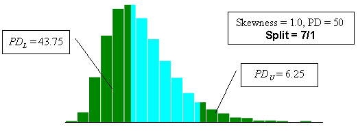
Figure 23a. Illustration of the divisions that SKEWBIAS2H uses to calculate bias in the PWL estimate for two-sided specification limits (skewness coefficient = +1.0, split=8/0).
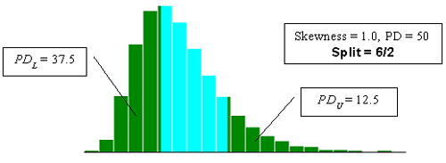
Figure 23b. Illustration of the divisions that SKEWBIAS2H uses to calculate bias in the PWL estimate for two-sided specification limits (skewness coefficient = +1.0, split=7/1).
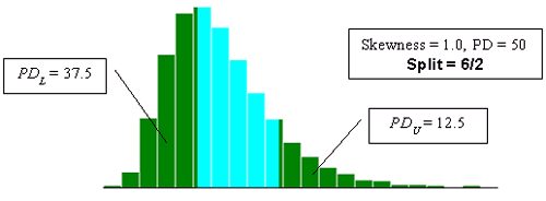
Figure 23c. Illustration of the divisions that SKEWBIAS2H uses to calculate bias in the PWL estimate for two-sided specification limits (skewness coefficient = +1.0, split=6/2).
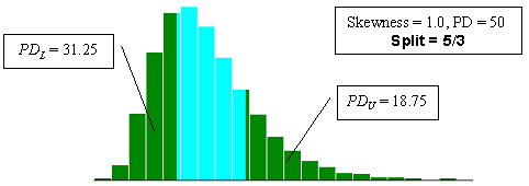
Figure 23d. Illustration of the divisions that SKEWBIAS2H uses to calculate bias in the PWL estimate for two-sided specification limits (skewness coefficient = +1.0, split=5/3).
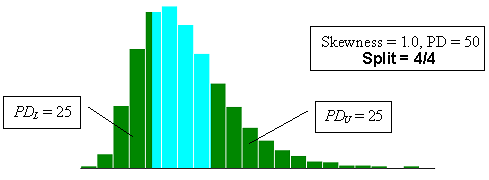
Figure 23e. Illustration of the divisions that SKEWBIAS2H uses to calculate bias in the PWL estimate for two-sided specification limits (skewness coefficient = +1.0, split=4/4).
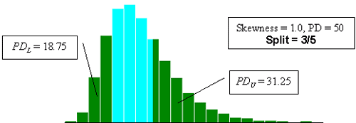
Figure 23f. Illustration of the divisions that SKEWBIAS2H uses to calculate bias in the PWL estimate for two-sided specification limits (skewness coefficient = +1.0, split=3/5).
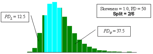
Figure 23g. Illustration of the divisions that SKEWBIAS2H uses to calculate bias in the PWL estimate for two-sided specification limits (skewness coefficient =+1.0, split = 2/6).
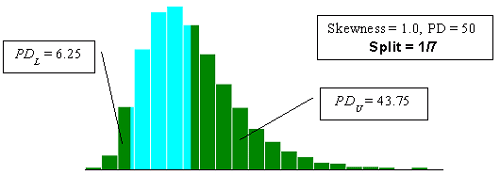
Figure 23h. Illustration of the divisions that SKEWBIAS2H uses to calculate bias in the PWL estimate for two-sided specification limits (skewness coefficient = +1.0, split = 1/7).
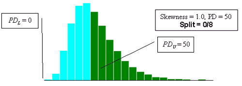
Figure 23i. Illustration of the divisions that SKEWBIAS2H uses to calculate bias in the PWL estimate for two-sided specification limits (skewness coefficient = +1.0, split = 0/8).
Tables 21 through 23 show simulation results that illustrate how the bias in estimating PD and, hence, PWL varies with the PDL/PDU division and sample size. In each analysis, 10,000 samples of the appropriate size were generated from a population with one of the skewness coefficients. The average bias and variability were then determined for the 10,000 PD estimates.
Figures 24 through 26 present plots of the results from tables 21 through 23, which indicate that the amount of bias in the PD estimate depends on the amount of skewness, the actual PD of the sampled population, the division of PDL/PDU, and the sample size used. Figures 27 through 29, which also plot the results from tables 21 through 23, highlight the effect of sample size on bias in the PD estimate.
As in the case of the one-sided specification limit shown earlier in this chapter, the larger the sample size, the greater the bias of the estimate. This probably stems from the fact that the larger sample does a better job of estimating PD for the assumed symmetrical normal distribution. This leads to a greater bias since the population is actually a skewed distribution rather than a symmetrical normal distribution.
To illustrate how this estimating bias arises for skewed distributions, figure 30 shows the plots of two populations-one that is normally distributed and one that has a skewness coefficient = +1.0. These two populations have the same mean, 5.0, and the same standard deviation, 1.0. The solid vertical line in the figure represents the mean for the two distributions. For the normal distribution, the median, or 50th percentile, occurs at the same value as the mean (i.e., 5.0). However, for the skewed distribution, the median is at a smaller value of 4.85.
Assume that the single lower specification limit is 5.0, meaning that the normal distribution has 50 PD (or 50 PWL). However, since the skewed distribution has a median of 4.85, it will have greater than 50 PD (or less than 50 PWL). Since the quality index is used to estimate PD (or PWL) and since this requires an assumption that the population is normally distributed, when the quality index determines an estimated PD of 50 for the normal distribution, the skewed distribution will have greater than 50 PD. Thus, for a population with 50 PD and for a single lower specification limit, if the skewness is away from the limit, the quality index will, on average, underestimate the PD value of the skewed distribution. If the skewness were in the direction of the lower specification limit, then the quality index would, on average, overestimate the PD value. This is exactly what is shown in figures 26 and 29. Appendix F shows additional simple illustrations of how biased estimates can be obtained.
Table 21. Results of simulations with PD = 10, 10,000 simulated lots, sample sizes = 3, 5, and 10, and two-sided limits.
| PDL/PDU | Skewness | ||||||
|---|---|---|---|---|---|---|---|
| 0.0 | 0.5 | 1.0 | 1.5 | 2.0 | 2.5 | 3.0 | |
| Sample Size = 3 | |||||||
| 8/0 | -0.22 | +0.05 | +0.73 | +1.83 | +2.14 | +3.20 | +3.80 |
| 7/1 | +0.27 | +0.14 | +0.63 | +1.34 | +2.13 | +3.24 | +3.87 |
| 6/2 | -0.14 | +0.01 | +1.03 | +1.25 | +2.61 | +3.33 | +4.09 |
| 5/3 | -0.05 | +0.12 | +0.77 | +1.89 | +2.67 | +3.87 | +4.74 |
| 4/4 | -0.07 | +0.15 | +1.07 | +1.64 | +3.58 | +4.25 | +5.43 |
| 3/5 | +0.02 | +0.14 | +0.86 | +2.17 | +2.97 | +4.52 | +5.54 |
| 2/6 | -0.15 | -0.03 | +1.13 | +2.03 | +3.58 | +4.79 | +6.59 |
| 1/7 | -0.01 | +0.43 | +0.89 | +1.94 | +3.68 | +5.31 | +6.51 |
| 0/8 | -0.13 | -0.06 | -0.13 | -0.05 | +0.40 | +0.11 | +0.31 |
| Sample Size = 5 | |||||||
| 8/0 | +0.07 | +0.71 | +1.56 | +2.70 | +3.63 | +4.58 | +5.64 |
| 7/1 | -0.02 | +0.45 | +1.44 | +2.32 | +3.43 | +4.81 | +5.78 |
| 6/2 | -0.29 | +0.20 | +1.41 | +2.46 | +3.81 | +4.19 | +6.39 |
| 5/3 | -0.23 | +0.21 | +1.48 | +2.68 | +4.47 | +5.74 | +6.82 |
| 4/4 | -0.02 | +0.36 | +1.76 | +3.27 | +4.66 | +6.20 | +7.77 |
| 3/5 | -0.36 | +0.27 | +1.80 | +3.43 | +5.47 | +7.14 | +8.28 |
| 2/6 | +0.13 | +0.50 | +1.79 | +3.79 | +5.61 | +7.75 | +9.76 |
| 1/7 | -0.01 | +0.59 | +1.98 | +3.47 | +6.19 | +8.46 | +10.03 |
| 0/8 | +0.11 | -0.26 | -0.36 | -0.18 | +0.45 | +0.45 | +0.64 |
| Sample Size = 10 | |||||||
| 8/0 | +0.05 | +0.92 | +2.22 | +3.57 | +5.07 | +6.27 | +7.40 |
| 7/1 | +0.06 | +0.56 | +1.76 | +3.26 | +4.94 | +6.26 | +7.58 |
| 6/2 | +0.11 | +0.42 | +1.66 | +3.31 | +5.03 | +6.65 | +8.25 |
| 5/3 | -0.16 | +0.46 | +1.87 | +3.64 | +5.69 | +7.52 | +8.90 |
| 4/4 | +0.07 | +0.50 | +2.10 | +3.97 | +6.13 | +8.03 | +9.77 |
| 3/5 | +0.07 | +0.60 | +2.24 | +4.40 | +6.53 | +8.79 | +10.93 |
| 2/6 | -0.08 | +0.68 | +2.37 | +4.96 | +7.27 | +9.77 | +11.91 |
| 1/7 | +0.14 | +0.53 | +2.46 | +5.32 | +7.88 | +10.77 | +12.77 |
| 0/8 | +0.02 | -0.61 | -0.69 | -0.21 | -0.10 | +0.43 | +1.18 |
Table 22. Results of simulations with PD = 30, 10,000 simulated lots, sample sizes = 3, 5, and 10, and two-sided limits.
| PDL/PDU | Skewness | ||||||
|---|---|---|---|---|---|---|---|
| 0.0 | 0.5 | 1.0 | 1.5 | 2.0 | 2.5 | 3.0 | |
| Sample Size = 3 | |||||||
| 8/0 | +0.11 | -0.49 | -0.86 | -1.34 | -1.46 | -1.33 | -1.36 |
| 7/1 | -0.08 | -0.64 | -0.61 | -1.01 | -1.01 | -1.13 | -1.37 |
| 6/2 | +0.18 | -0.36 | -0.68 | -0.48 | -0.53 | -0.01 | +0.12 |
| 5/3 | -0.28 | +0.13 | +0.14 | +0.40 | +0.60 | +1.01 | +1.94 |
| 4/4 | +0.34 | -0.37 | +0.81 | +1.37 | +1.73 | +2.30 | +3.67 |
| 3/5 | -0.04 | +0.63 | +1.07 | +2.15 | +2.73 | +3.75 | +4.46 |
| 2/6 | -0.40 | +0.64 | +1.86 | +3.05 | +4.18 | +5.50 | +6.67 |
| 1/7 | -0.47 | +0.59 | +2.12 | +3.66 | +5.46 | +7.58 | +8.19 |
| 0/8 | +0.03 | +0.27 | +0.78 | +1.19 | +1.84 | +2.10 | +2.67 |
| Sample Size = 5 | |||||||
| 8/0 | -0.07 | -0.84 | -1.96 | -2.26 | -2.69 | -2.94 | -3.08 |
| 7/1 | +0.35 | -1.36 | -2.02 | -2.46 | -2.52 | -2.61 | -2.32 |
| 6/2 | +0.13 | -0.75 | -1.31 | -1.27 | -1.06 | -0.56 | -0.27 |
| 5/3 | +0.20 | -0.50 | -0.66 | -0.01 | +1.04 | +1.48 | +1.80 |
| 4/4 | +0.04 | +0.18 | +0.88 | +2.04 | +2.75 | +4.08 | +5.25 |
| 3/5 | -0.02 | +0.61 | +1.97 | +3.61 | +5.10 | +6.63 | +7.79 |
| 2/6 | -0.26 | +1.17 | +3.19 | +5.18 | +7.25 | +9.28 | +11.22 |
| 1/7 | +0.02 | +1.87 | +3.99 | +7.05 | +9.18 | +12.10 | +14.07 |
| 0/8 | -0.03 | +1.18 | +1.81 | +3.69 | +4.31 | +5.27 | +5.99 |
| Sample Size = 10 | |||||||
| 8/0 | +0.03 | -1.44 | -2.40 | -3.14 | -3.56 | -3.63 | -3.53 |
| 7/1 | +0.12 | -2.01 | -2.97 | -3.34 | -3.36 | -3.04 | -2.80 |
| 6/2 | +0.07 | -1.28 | -2.21 | -1.83 | -1.24 | -0.57 | +0.45 |
| 5/3 | -0.10 | -0.75 | -0.43 | +0.36 | +1.36 | +2.59 | +3.83 |
| 4/4 | -0.01 | +0.33 | +1.28 | +2.57 | +4.55 | +6.19 | +8.34 |
| 3/5 | +0.06 | +1.11 | +3.08 | +5.29 | +7.73 | +10.08 | +12.51 |
| 2/6 | -0.23 | +2.13 | +5.13 | +7.98 | +10.88 | +13.38 | +15.99 |
| 1/7 | -0.01 | +2.59 | +6.44 | +10.01 | +13.97 | +16.84 | +19.92 |
| 0/8 | +0.16 | +1.56 | +3.35 | +5.40 | +6.80 | +8.17 | +9.70 |
Table 23. Results of simulations with PD = 50, 10,000 simulated lots, sample sizes = 3, 5, and 10, and two-sided limits.
| PDL/PDU | Skewness | ||||||
|---|---|---|---|---|---|---|---|
| 0.0 | 0.5 | 1.0 | 1.5 | 2.0 | 2.5 | 3.0 | |
| Sample Size = 3 | |||||||
| 8/0 | -0.08 | -0.82 | -1.37 | -2.29 | -3.12 | -3.38 | -3.40 |
| 7/1 | -0.39 | -0.94 | -1.77 | -2.11 | -2.39 | -3.13 | -3.11 |
| 6/2 | +0.41 | -0.67 | -1.42 | -1.64 | -1.59 | -2.45 | -2.33 |
| 5/3 | +0.05 | -0.48 | -0.40 | -0.77 | -0.48 | -0.60 | +0.08 |
| 4/4 | +0.13 | -0.15 | +0.59 | +0.55 | +1.00 | +1.47 | +1.96 |
| 3/5 | +0.25 | +0.44 | +0.97 | +1.97 | +2.56 | +2.97 | +4.16 |
| 2/6 | -0.04 | +1.12 | +1.69 | +2.91 | +4.14 | +5.32 | +5.71 |
| 1/7 | -0.12 | +1.38 | +2.64 | +3.86 | +5.23 | +6.80 | +8.22 |
| 0/8 | +0.05 | +0.87 | +1.41 | +1.99 | +2.92 | +3.03 | +4.11 |
| Sample Size = 5 | |||||||
| 8/0 | -0.15 | -1.44 | -3.06 | -4.67 | -5.64 | -6.45 | -7.55 |
| 7/1 | -0.01 | -2.15 | -3.56 | -4.90 | -5.80 | -6.24 | -6.57 |
| 6/2 | +0.06 | -1.39 | -2.70 | -3.46 | -3.79 | -3.97 | -3.97 |
| 5/3 | +0.25 | -1.16 | -1.07 | -1.11 | -0.86 | -0.60 | -0.34 |
| 4/4 | -0.19 | -0.04 | +0.48 | +1.17 | +2.28 | +2.91 | +3.74 |
| 3/5 | +0.03 | +0.89 | +2.22 | +3.53 | +5.00 | +6.51 | +7.51 |
| 2/6 | -0.02 | +1.73 | +3.88 | +6.27 | +8.03 | +9.95 | +11.50 |
| 1/7 | 0.00 | +2.41 | +5.30 | +8.06 | +10.93 | +12.89 | +15.06 |
| 0/8 | +0.07 | +1.65 | +3.17 | +4.57 | +5.42 | +6.41 | +7.43 |
| Sample Size = 10 | |||||||
| 8/0 | -0.07 | -2.26 | -4.66 | -6.69 | -8.06 | -9.33 | -9.98 |
| 7/1 | -0.17 | -3.22 | -5.56 | -6.96 | -8.20 | -8.83 | -9.08 |
| 6/2 | +0.15 | -2.22 | -3.78 | -4.69 | -4.71 | -4.90 | -4.67 |
| 5/3 | +0.26 | -1.01 | -1.56 | -1.31 | -0.48 | +0.41 | +0.94 |
| 4/4 | +0.17 | +0.04 | +1.15 | +2.38 | +4.09 | +5.65 | +6.74 |
| 3/5 | -0.01 | +1.41 | +3.70 | +5.56 | +8.17 | +10.36 | +12.33 |
| 2/6 | 0.00 | +2.62 | +5.93 | +8.88 | +11.84 | +14.59 | +17.13 |
| 1/7 | -0.05 | +3.48 | +7.56 | +11.71 | +15.36 | +18.38 | +20.71 |
| 0/8 | -0.08 | +2.34 | +4.93 | +6.61 | +8.03 | +9.35 | +10.39 |
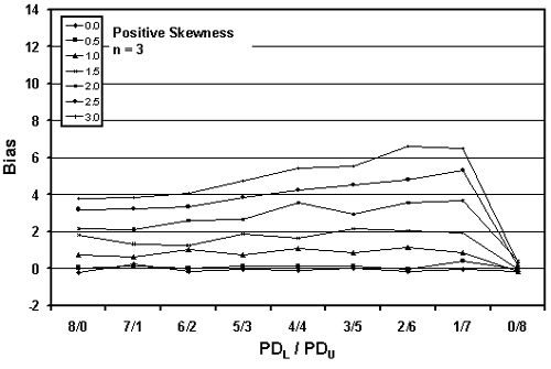
Figure 24a. Plot of bias versus PDL/PDU divisions for 10,000 simulated lots with PD = 10, sample = 3, and two-sided limits.
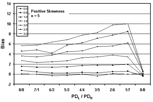
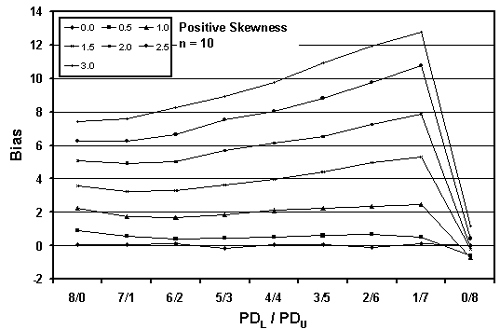
Figure 24c. Plot of bias versus PDL/PDU divisions for 10,000 simulated lots with PD = 10, sample = 10, and two-sided limits.
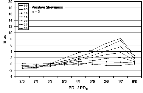
Figure 25a. Plot of bias versus PDL/PDU divisions for 10,000 simulated lots with PD = 30, sample = 3, and two-sided limits.
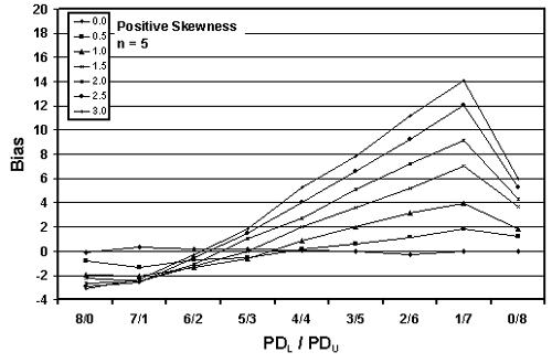
Figure 25b. Plot of bias versus PDL/PDU divisions for 10,000 simulated lots with PD = 30, sample = 5, and two-sided limits.
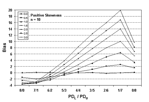
Figure 25c. Plot of bias versus PDL/PDU divisions for 10,000 simulated lots with PD = 30, sample = 10, and two-sided limits.
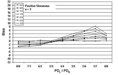
Figure 26a. Plot of bias versus PDL/PDU divisions for 10,000 simulated lots with PD = 50, sample = 3 and two-sided limits.
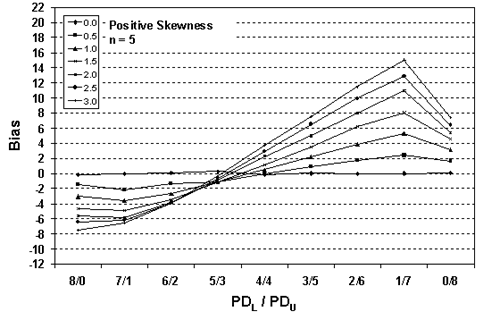
Figure 26b. Plot of bias versus PDL/PDU divisions for 10,000 simulated lots with PD = 50, sample = 5, and two-sided limits.
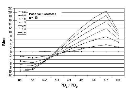
Figure 26c. Plot of bias versus PDL/PDU divisions for 10,000 simulated lots with PD = 50, sample = 10, and two-sided limits.
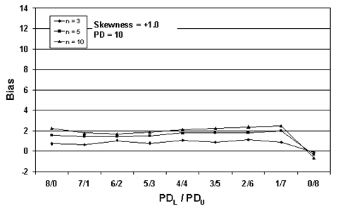
Figure 27a. Plot of bias versus SKEWBIAS2H divisions for 10,000 simulated lots with PD = 10, skewness = 1, and two-sided limits.
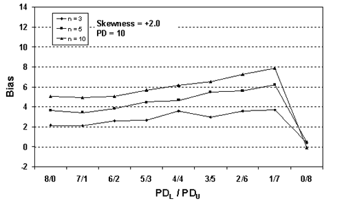
Figure 27b. Plot of bias versus SKEWBIAS2H divisions for 10,000 simulated lots with PD = 10, skewness = 2, and two-sided limits.
Figure 28a. Plot of bias versus SKEWBIAS2H divisions for 10,000 simulated lots with PD = 30, skewness = 1, and two-sided limits.
Figure 28b. Plot of bias versus SKEWBIAS2H divisions for 10,000 simulated lots with PD = 30, skewness = 2, and two-sided limits.
Figure 29a. Plot of bias versus SKEWBIAS2H divisions for 10,000 simulated lots with PD = 50, skewness = 1, and two-sided limits.
Figure 29b. Plot of bias versus SKEWBIAS2H divisions for 10,000 simulated lots with PD = 50, skewness = 2, and two-sided limits.
Figure 30. Comparison of a normal population with a population with skewness coefficient = +1.0.
Variability of PWL/PD Estimates: Simulation was also used to evaluate the variability of PD estimates and to show how sample size affects this variability. Figure 31 shows an example of an output screen for a normal population (i.e., skewness coefficient = 0.00) that actually has a PD = 10 and sample size = 5. The results of the nine divisions for PDL/PDU are clearly indicated.
The BIAS/SE results indicate the average bias and the standard error of the bias, respectively. The bias values are relatively closely distributed about zero, indicating that the method for estimating PD (and, hence, PWL) is not biased for a symmetrical distribution. This is to be expected since the PD estimating method assumes a symmetrical normal distribution.
The standard error values for sample size n = 5 are all 0.11. The standard error is determined by calculating the standard deviation of the 10,000 lot sample means and then dividing this standard deviation by the square root of 10,000 (i.e., the number of sample averages). The standard error is a measure of the variability of the estimate for the population mean. The standard error is not a measure of the variability of the individual lot sample means. However, it can be related to this individual sample mean variability.
Table 8 shows the standard deviation values calculated from 1000 sample means. If the standard deviation values in table 8 were taken as estimates for the variability of the individual sample means, then these values would estimate the standard error values in figure 31 by dividing the table 8 values by the square root of 10,000, which is 100. The value in table 8 for a population with 90 PWL, which corresponds to 10 PD in figure 31, is 11.42. If you divide this number by 100, the result is 0.1142, which is consistent with the standard error of 0.11 shown in figure 31.
Figure 32 shows portions of the output from three simulations, each with a population of PD = 10 and skewness coefficient = 0.00. In the figure, the divisions for 8/0, 7/1, and 6/2 are shown for sample sizes = 3, 5, and 10. These histograms represent the individual bias values for the 10,000 lots that were simulated.
One thing is immediately apparent-the bias plots are not symmetrical. This is because of the natural boundaries of 0 PD and 100 PD. It is not possible to have less than 0 PD, so it is not possible to have a bias estimate of less than -10 PD. It is possible, however, to overestimate PD by as much as +90 PD. This is reflected in the plots that are skewed to the right, while having no bias values of less than -10. The second point to notice in the plots is that the variability of the bias results is related to sample size. This is shown in the standard error values and in the spread of the histogram plots. The larger the sample size, the smaller the standard error and the less spread there is in the bias histogram.
As already shown in tables and figures above, the bias values vary with the amount of skewness, the sample size, the PD or PWL of the population, and the division of PD material outside the upper and lower specification limits. Figure 32 shows that the shape and the spread of the distribution of the sample means vary with the sample size. These distributions also vary in shape considerably with the population PD or PWL value. Appendix G contains a number of sample output screens that illustrate the shape and spread of the sample means for a variety of sample sizes and population PD values.
While appendix G contains populations with skewness coefficients up to 3.00, in practice, it is unlikely that highway materials will have skewness values much greater than 1.00. Figure 33 shows an example of an output screen for a population with a skewness coefficient = 1.00 that has a PD = 30 and sample size = 5. Figure 34 shows portions of the output screens for the same population, but with sample sizes = 3, 5, and 10.
Figure 31. Sample program output screen for a population with PD = 10, skewness coefficient = 0.00, and sample size = 5.
Figure 32a. Portions of program output screen for PD = 10, skewness coefficient = 0.00, sample = 3.
Figure 32b. Portion of program output screens for PD = 10, skewness coefficient = 0.00, sample = 5.
Figure 32c. Portion of program output screens for PD = 10, skewness coefficient = 0.00, sample = 10.
Figure 33. Sample program output screen for a population with PD = 30, skewness coefficient = 1.00, and sample size = 5.
Figure 34a. Portion of program output screens for PD = 30, skewness coefficient = 1.00, and sample = 3.
Figure 34b. Portion of program output screens for PD = 30, skewness coefficient = 1.00, and sample = 5.
Figure 34c. Portion of program output screens for PD = 30, skewness coefficient = 1.00, and sample = 10.
A computer simulation program was developed to investigate the performance of the AAD estimating procedures when working with a skewed distribution. The program can generate a population with any mean and standard deviation, and with skewness coefficients for distributions that are symmetrical (0.0), negatively skewed (-3.0, -2.5, -2.0, -1.5, -1.0, -0.5), or positively skewed (+3.0, +2.5, +2.0, +1.5, +1.0, +0.5). The program determines the actual AAD for the population with the input values for mean, standard deviation, skewness coefficient, and offset of the mean from the target value. The program then generates 10,000 samples from the input distribution and determines the estimated AAD for each sample. The sample size can be 3 to 30 values per sample. The program then determines the mean, standard deviation, standard error, minimum value, and maximum value for the 10,000 AAD values. It also prints a histogram for the generated AAD values.
Figure 35 shows the effect of a skewed population on the actual population AAD for populations that are centered on the target value and that have skewness coefficients ranging from 0.0 to +3.0 in increments of 0.5. The actual AAD values would be the same for negative skewness coefficients of the same magnitude as long as the population means were centered on the target. Since the population means are centered on the target values, the population AAD values actually decrease as the populations become more skewed.
Figure 36 shows the effect of sample sizes = 3, 5, and 10 on the sampling distributions for the AAD estimates for populations that are centered on the target value and that have skewness coefficients of 0.0, +0.5, and +1.0. As would be expected, the spread of the AAD estimates decreases as the sample size increases. This is reflected in the reduced spread in the histogram plots and in the smaller standard deviation values as the sample size increases. It also appears that the mean of the sampling distribution approximates the actual population AAD value quite well regardless of the level of skewness in the population.
Figure 37 shows three populations with the same standard deviation, but with mean offsets from the target = 0.0, 1.0, and 2.0. These mean offsets are measured in standard deviation units. As would be expected, the actual population AAD increases as the mean moves away from the target value. The mean of the estimated AAD values is quite close to the actual values regardless of the mean offset. However, the standard deviation (i.e., the spread) of the AAD sample values increases as the mean offset increases.
Figure 38 shows three populations that have extremely different distributions, but which all have essentially equal AAD values. Although the means of the sampling distributions are about the same, the skewed distributions have greater spread in the AAD values for individual lots. It is not certain, but it seems unlikely that each of these populations would perform identically in service, even though they have the same population AAD values.
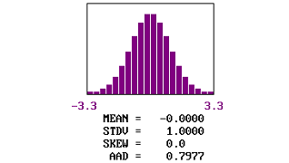
Figure 35a. Example of AAD distribution and actual values for populations centered on the target and with skewness coefficient of 0.
Figure 35b. Examples of AAD distribution and actual values for populations centered on the target and with skewness coefficients between .5 and 1.5.
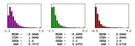
Figure 35c. Examples of AAD distribution and actual values for populations centered on the target and with skewness coefficients between 2.0 and 3.0.
Figure 36a. Comparison of the shapes and spread of estimated AAD values for populations centered on the target and with various skewness coefficients.
Figure 36b. Comparison of the shapes and spread of estimated AAD values for populations centered on the target and with various skewness coefficients, sample size=3.
Figure 36c. Comparison of the shapes and spread of estimated AAD values for populations centered on the target and with various skewness coefficients, sample size = 5.
Figure 36d. Comparison of the shapes and spread of estimated AAD values for populations centered on the target and with various skewness coefficients, sample size = 10.
Figure 37. Comparison of the shapes and spread of estimated AAD values for normal populations centered on and offset from the target.
Figure 38. Example of populations that are very dissimilar in shape, but have approximately the same AAD.
There are obviously an infinite number of combinations of population mean offsets from the target and skewness coefficients. It is not possible to evaluate all of these combinations. However, it is possible to hold the others constant and change only one variable to see what effect this might have.
For sample sizes = 3, 5, and 10, table 24 lists the actual AAD values, the mean of the AAD sample values (i.e., the bias), and the standard deviation values for a number of populations that are all centered on the target, but have varying skewness levels. Figure 39 plots the results from table 24. It is apparent that the means of the AAD sample estimates are generally close to the true AAD values. In other words, the AAD estimating process appears to be unbiased. However, the standard deviations of the AAD sample estimates increase as the skewness level increases, while they decrease with increasing sample size.
For a sample size = 5, table 25 lists the actual AAD values, the mean of the AAD sample values (i.e., the bias), and the standard deviation values for a number of normal populations (i.e., skewness coefficient = 0.0) with centers that vary with respect to the amount of their offset from the target. Figure 40 plots the results from table 25. It is apparent that the means of the AAD sample estimates are generally close to the true AAD values. In other words, the AAD estimating process appears to be unbiased. However, the standard deviations of the AAD sample estimates increase as the mean offset from the target increases.
For a sample size = 5, table 26 lists the actual AAD values, the mean of the AAD sample values (i.e., the bias), and the standard deviation values for a number of normal populations that are all centered on the target, but with varying population standard deviation values. Figure 41 plots the results from table 26. It is apparent that the means of the AAD sample estimates are generally close to the true AAD values. In other words, the AAD estimating process appears to be unbiased. However, the standard deviations of the AAD sample estimates increase as the population standard deviation increases.
Table 24. Bias and spread of the AAD sample estimates for populations centered on the target, but with various levels of skewness.
| n | Offset | Skewness | Std. Dev. | AAD | Bias | Std. Dev. of AAD Values |
|---|---|---|---|---|---|---|
| 3 | 0.00 | 0.00 | 1.00 | 0.7977 | 0.0042 | 0.3502 |
| 0.50 | 0.7934 | 0.0048 | 0.3524 | |||
| 1.00 | 0.7776 | 0.0081 | 0.3659 | |||
| 1.50 | 0.7544 | 0.0013 | 0.3783 | |||
| 2.00 | 0.7273 | -0.0067 | 0.3997 | |||
| 2.50 | 0.6993 | 0.0061 | 0.4202 | |||
| 3.00 | 0.6718 | -0.0047 | 0.4158 | |||
| 5 | 0.00 | 0.00 | 1.00 | 0.7977 | 0.0004 | 0.2693 |
| 0.50 | 0.7934 | 0.0007 | 0.2709 | |||
| 1.00 | 0.7776 | -0.0008 | 0.2811 | |||
| 1.50 | 0.7544 | -0.0026 | 0.2908 | |||
| 2.00 | 0.7273 | -0.0012 | 0.3064 | |||
| 2.50 | 0.6993 | -0.0041 | 0.3136 | |||
| 3.00 | 0.6718 | -0.0023 | 0.3316 | |||
| 10 | 0.00 | 0.00 | 1.00 | 0.7977 | -0.0009 | 0.1899 |
| 0.50 | 0.7934 | -0.0022 | 0.1919 | |||
| 1.00 | 0.7776 | 0.0018 | 0.1975 | |||
| 1.50 | 0.7544 | 0.0009 | 0.2069 | |||
| 2.00 | 0.7273 | 0.0036 | 0.2191 | |||
| 2.50 | 0.6993 | -0.0012 | 0.2233 | |||
| 3.00 | 0.6718 | 0.0009 | 0.2334 |
n = sample size, tests per lot
Offset = offset of population mean from the target value, in units of standard deviation
Skewness = skewness coefficient for the population
Std. Dev. = standard deviation for the population
AAD = actual AAD value for the population
Bias = average of the estimated AAD values minus the actual AAD value
Std. Dev. of AAD Values = standard deviation of the estimated AAD values
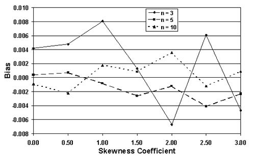
Figure 39a. Bias of the AAD sample estimates for populations centered on the target, but with various levels of skewness.
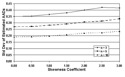
Figure 39b. Spread of the AAD sample estimates for populations centered on the target, but with various levels of skewness.
Table 25. Bias and spread of the AAD sample estimates for normal populations with various offsets from the target and n = 5.
| n | Offset | Skewness | Std. Dev. | AAD | Bias | Std. Dev. of AAD Values |
|---|---|---|---|---|---|---|
| 5 | 0.00 | 0.00 | 1.00 | 0.7977 | -0.0014 | 0.2682 |
| 0.25 | 0.8225 | -0.0014 | 0.2808 | |||
| 0.50 | 0.8955 | 0.0012 | 0.3000 | |||
| 0.75 | 1.0123 | 0.0003 | 0.3258 | |||
| 1.00 | 1.1666 | 0.0020 | 0.3590 | |||
| 1.25 | 1.3511 | -0.0030 | 0.3866 | |||
| 1.50 | 1.5585 | 0.0037 | 0.4027 | |||
| 1.75 | 1.7822 | 0.0007 | 0.4227 | |||
| 2.00 | 2.0168 | 0.0024 | 0.4280 |
n = sample size, tests per lot
Offset = offset of population mean from the target value, in units of standard
deviation Skewness = skewness coefficient for the population
Std. Dev. = standard deviation for the population
AAD = actual AAD value for the population
Bias = average of the estimated AAD values minus the actual AAD value
Std. Dev. of AAD Values = standard deviation of the estimated AAD values
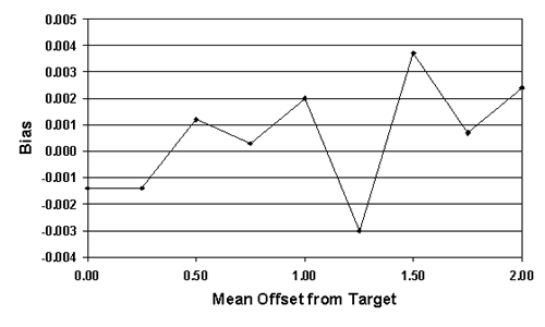
Figure 40a. Bias of the AAD samples estimates for normal populations with various offsets from the target and n=5.

Figure 40b. Spread of the Estimated AAD sample estimates for normal populations with various offsets from the target and n = 5.
Table 26. Bias and spread of the AAD sample estimates for normal populations with various standard deviation values and n = 5.
| n | Offset | Skewness | Std. Dev. | AAD | Bias | Std. Dev. of AAD Values |
|---|---|---|---|---|---|---|
| 5 | 0.00 | 0.00 | 1.00 | 0.7977 | 0.0014 | 0.2683 |
| 1.25 | 0.9971 | 0.0010 | 0.3328 | |||
| 1.50 | 1.1965 | -0.0011 | 0.4037 | |||
| 1.75 | 1.3960 | 0.0015 | 0.4784 | |||
| 2.00 | 1.5954 | -0.0037 | 0.5358 | |||
| 2.25 | 1.7948 | -0.0007 | 0.6050 | |||
| 2.50 | 1.9942 | 0.0055 | 0.6773 | |||
| 2.75 | 2.1936 | 0.0001 | 0.7341 | |||
| 3.00 | 2.3931 | 0.0012 | 0.8164 |
n = sample size, tests per lot
Offset = offset of population mean from the target value, in units of standard deviation
Skewness = skewness coefficient for the population
Std. Dev. = standard deviation for the population
AAD = actual AAD value for the population
Bias = average of the estimated AAD values minus the actual AAD value
Std. Dev. of AAD Values = standard deviation of the estimated AAD values
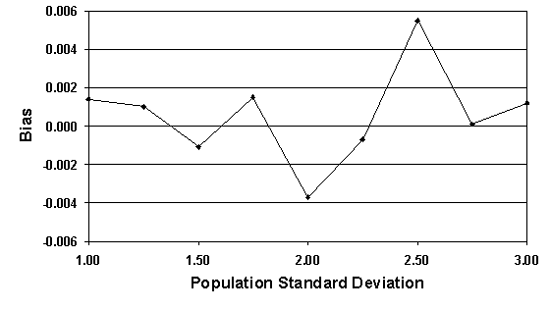
Figure 41a. Bias of the AAD sample estimates for normal populations centered on the target, with various standard deviation values, and n=5.
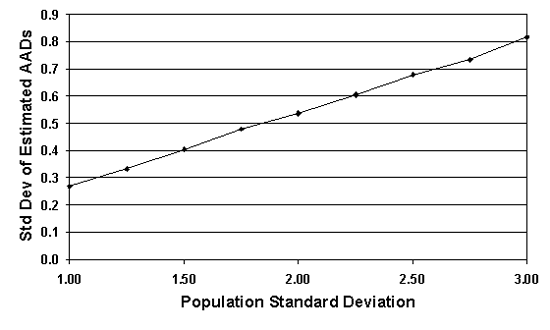
Figure 41b. Standard Deviation of the AAD sample estimates for normal populations centered on the target, with various standard deviation values, and n = 5.
Both PWL and AAD seemed to perform reasonably well when used with skewed distributions. They both provided bias estimates that were close to the actual values. They both had decreasing variability of the estimated values as the sample size increased. They both had increasing variability of the estimated values as the departures from normality became more pronounced.
However, it is difficult to compare the performance of the two since the magnitude of the numbers that are calculated varies so greatly. The PWL (or PD) values can range from 0 to 100, whereas AAD values will typically range from 0 to a value of less than 10. Also, if the PWL and AAD results were to be converted to payment factors by some equation, the multiplier for the AAD equation is likely to be much larger than the one for the PWL equation.
While no definitive conclusion can be drawn, both methods will probably provide satisfactory results for the amount of skewness that is likely to be found in highway materials applications.
It is possible that a process that is believed to be normally distributed could change, thereby resulting in a bimodal distribution. This could happen, for instance, if the asphalt content was changed at a mixing plant and the data from before and after the change were considered in the same lot calculations. Another way in which a bimodal distribution could appear is if there were two different plants providing materials for the same project. If the plants had different process means, then the combined output from the two plants might result in a bimodal distribution.
A computer simulation program was developed to investigate the performance of the PWL estimating procedures when working with a bimodal distribution. The program forms a bimodal distribution in the same manner in which it would happen in actual practice-by combining two different normal populations. The output screen for the program provides a plot of the distribution of each of the individual populations and a plot for the combined distribution.
When two populations are combined, they can differ in three ways:
The program can handle any of these three situations. Each of these three scenarios is considered in the following sections:
Different Means: A sample output screen from the program is shown in figure 42. In this example, two identical populations are combined. Each population, shown as Distribution #1 and Distribution #2 in figure 42, has a mean of 10.00 and a standard deviation of 1.00. Each population also has a PD of 9.99. The top two plots in figure 42 represent these populations. The combined population has a mean = 10.00, standard deviation = 1.00, and PD = 9.99. Figure 42 also shows the lower specification limit, Limit1, to be 8.72 and the upper specification limit, Limit2, to be 999.00. These limits are input by the user. Inputting a very large upper limit that will never be reached makes this an example for a specification item that has only a lower limit. By trial and error, input limits can be easily developed to represent any value for the population PD (or PWL) value. The bottom plot in figure 42 represents the combined population.
The right side of the screen shows the results of the simulation of, in this example, 1000 replications of a sample size = 5. The average of these 1000 sample PD values is shown as 10.16, with a standard deviation of 11.46. A histogram of the differences between the individual sample PD values and the true population PD value is also shown. In the bottom right corner of the screen, Summary of Results shows that the PD bias was 0.16 and that we are 95-percent confident that the true value falls within the range of 0.16 ±0.71.
It is to be expected that if two identical distributions are combined, the result will be the same distribution. What will happen then if distributions with different means, but the same standard deviations, are combined? Figure 43 shows, for a sample size = 5, the output screens for cases where the offset between the population means varies from 1 to 5 standard deviations. Note that for 1 and 2 standard deviation offsets, the combined populations still appear to be approximately normal. Not until the mean offset reaches 3 does the bimodal shape begin to become apparent. It is unlikely that distributions that are so different would be combined, and if they were combined, problems would probably arise that would make the error obvious. This means that for most practical cases, if two distributions with the same standard deviation were combined, the combined distribution would not differ enough from normal to adversely affect the PD or PWL estimates.
Table 27 presents the results of simulation analyses in which two distributions with equal standard deviations and a variety of mean offsets were combined. This table represents the case of a single specification limit. Table 28 provides similar results for simulation analyses of two-sided specifications. The tables indicate that the average bias values are reasonably small, particularly for mean offsets of up to 2 or 3 standard deviations.
Different Standard Deviations: The combining of two normal distributions with different standard deviations, but with equal means, presents no different situation with respect to estimating PWL than does a single normal distribution. This is because whenever two normal distributions with equal means are combined, the resulting distribution will always be another normal distribution, regardless of the values of their standard deviations. This is illustrated in figure 44, which shows example output screens in which several pairs of normal distributions with differing standard deviations are combined. The resulting combined distribution always has the same mean as the two initial distributions and the only difference is the standard deviation for the combined distribution. Therefore, no additional discussion is necessary for the case of combining normal distributions with equal means.
Figure 42. Sample output screen from the simulation program for bimodal distributions.
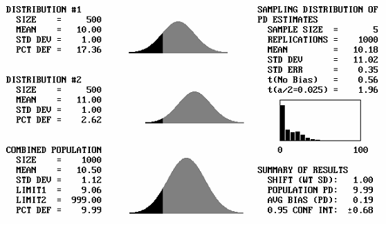
Figure 43a. Program output screens for sample size = 5 and mean offsets = 1.
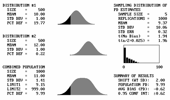
Figure 43b. Program output screens for sample size = 5 and mean offsets = 2.
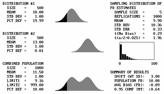
Figure 43c. Program output screens for sample size = 5 and mean offsets = 3.
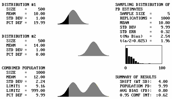
Figure 43d. Program output screens for sample size = 5 and mean offsets = 4.
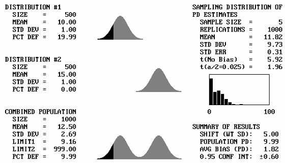
Figure 43e. Program output screens for sample size = 5 and mean offsets = 5.
Table 27. Bias results for combining two populations with equal σ with one-sided limits.
| n | Offset | Actual PD | Average PD | Average Bias | 95% CI | Different? |
|---|---|---|---|---|---|---|
| 5 | 0.0 | 9.99 | 10.16 | +0.16 | ±0.71 | N |
| 5 | 1.0 | 9.99 | 10.18 | +0.19 | ±0.68 | N |
| 5 | 2.0 | 9.99 | 9.37 | -0.62 | ±0.62 | N |
| 5 | 3.0 | 10.00 | 9.90 | -0.09 | ±0.64 | N |
| 5 | 4.0 | 9.99 | 10.80 | +0.80 | ±0.62 | S |
| 5 | 5.0 | 9.99 | 11.82 | +1.82 | ±0.60 | S |
| 3 | 0.0 | 9.99 | 10.00 | +0.01 | ±0.97 | N |
| 3 | 1.0 | 9.99 | 10.32 | +0.33 | ±0.94 | N |
| 3 | 2.0 | 9.99 | 9.25 | -0.74 | ±0.89 | N |
| 3 | 3.0 | 10.00 | 9.74 | -0.26 | ±0.88 | N |
| 3 | 4.0 | 9.99 | 10.57 | +0.58 | ±0.92 | N |
| 3 | 5.0 | 9.99 | 11.85 | +1.86 | ±0.89 | S |
| 5 | 0.0 | 30.02 | 29.62 | -0.39 | ±1.05 | N |
| 5 | 1.0 | 30.01 | 29.25 | -0.75 | ±1.06 | N |
| 5 | 2.0 | 30.01 | 27.27 | -1.74 | ±1.09 | S |
| 5 | 3.0 | 30.01 | 26.40 | -3.61 | ±0.99 | S |
| 5 | 4.0 | 30.00 | 24.67 | -5.33 | ±0.99 | S |
| 5 | 5.0 | 30.01 | 23.17 | -6.84 | ±0.94 | S |
| 3 | 0.0 | 30.02 | 29.91 | -0.10 | ±1.54 | N |
| 3 | 1.0 | 30.01 | 29.81 | -0.20 | ±1.52 | N |
| 3 | 2.0 | 30.01 | 30.38 | +0.37 | ±1.45 | N |
| 3 | 3.0 | 30.01 | 27.39 | -2.62 | ±1.44 | S |
| 3 | 4.0 | 30.00 | 26.63 | -3.37 | ±1.36 | S |
| 3 | 5.0 | 30.01 | 25.47 | -4.54 | ±1.34 | S |
n = sample size
Offset = offset of the two population means in terms of the average σ of the populations
Actual PD = actual percent defective (PD) of the combined population
Average PD = average PD of 1000 simulated samples from the combined population
Average Bias = average simulated PD minus the actual PD
95% CI = interval within which 95 percent of the average bias values should fall
Different? = whether or not the average bias is significantly different from zero at the
0.05 level (N = not significantly different, S = significantly different)
Table 28. Bias results for combining two populations with equal σ with two-sided limits equidistant from the mean.
| n | Offset | Actual PD | Average PD | Average Bias | 95% CI | Different? |
|---|---|---|---|---|---|---|
| 5 | 0.0 | 10.00 | 9.38 | -0.61 | ±0.66 | N |
| 5 | 1.0 | 10.00 | 10.21 | +0.21 | ±0.66 | N |
| 5 | 2.0 | 9.99 | 10.47 | +0.48 | ±0.66 | N |
| 5 | 3.0 | 9.99 | 12.46 | +2.47 | ±0.63 | S |
| 5 | 4.0 | 9.99 | 14.51 | +4.52 | ±0.59 | S |
| 5 | 5.0 | 9.99 | 16.40 | +6.41 | ±0.57 | S |
| 3 | 0.0 | 10.00 | 10.70 | +0.71 | ±0.98 | N |
| 3 | 1.0 | 10.00 | 10.33 | +0.34 | ±0.94 | N |
| 3 | 2.0 | 9.99 | 10.98 | +0.99 | ±0.96 | S |
| 3 | 3.0 | 9.99 | 11.30 | +1.31 | ±0.91 | S |
| 3 | 4.0 | 9.99 | 13.06 | +3.07 | ±0.90 | S |
| 3 | 5.0 | 9.99 | 11.30 | +1.31 | ±0.91 | S |
| 5 | 0.0 | 30.02 | 29.83 | -0.19 | ±1.03 | N |
| 5 | 1.0 | 30.02 | 30.05 | +0.03 | ±0.99 | N |
| 5 | 2.0 | 30.02 | 28.77 | -1.24 | ±0.93 | S |
| 5 | 3.0 | 30.00 | 27.23 | -2.77 | ±0.81 | S |
| 5 | 4.0 | 30.02 | 28.90 | -1.12 | ±0.70 | S |
| 5 | 5.0 | 30.02 | 29.03 | -0.99 | ±0.59 | S |
| 3 | 0.0 | 30.02 | 30.14 | +0.12 | ±1.54 | N |
| 3 | 1.0 | 30.02 | 28.80 | -1.21 | ±1.52 | N |
| 3 | 2.0 | 30.02 | 28.33 | -1.69 | ±1.45 | S |
| 3 | 3.0 | 30.00 | 29.89 | -0.11 | ±1.44 | N |
| 3 | 4.0 | 30.02 | 29.61 | -0.42 | ±1.36 | N |
| 3 | 5.0 | 30.02 | 30.71 | +0.70 | ±1.34 | N |
n = sample size
Offset = offset of the two population means in terms of the average σ of the populations
Actual PD = actual percent defective (PD) of the combined population
Average PD = average PD of 1000 simulated samples from the combined population
Average Bias = average simulated PD minus the actual PD
95% CI = interval within which 95 percent of the average bias values should fall
Different? = whether or not the average bias is significantly different from zero at the 0.05 level (N = not significantly different, S = significantly different)
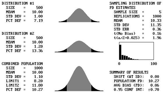
Figure 44a. Illustration 1 of program output screens when combining distributions with equal means for sample size = 5.
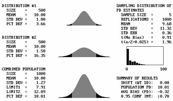
Figure 44b. Illustration 2 of program output screens when combining distributions with equal means for sample size = 5.
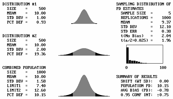
Figure 44c. Illustration 3 of program output screens when combining distributions with equal means for sample size = 5.
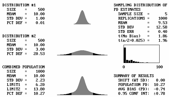
Figure 44d. Illustration 4 of program output screens when combining distributions with equal means for sample size = 5.
Different Means and Different Standard Deviations: When populations with different means and different standard deviations are combined, the shape of the combined distribution depends on the amount of difference between them. This is illustrated in the combined distribution shapes in table 29. The original distributions in this figure are different in both mean and standard deviation. The ratio of the standard deviations of the two populations is 2.0. The offset of the two means is stated in terms of the weighted standard deviation. This is simply the arithmetic average of the standard deviations for the two distributions that are combined.
For small offsets, the combined distribution is simply a unimodal skewed distribution. It is not until the weighted offset reaches 2.0 that a slight bulge appears in the long tail of the skewed distribution. This bulge becomes more distinct and the combined distribution approaches a true bimodal shape as the weighted offset increases to above 3.0.
To investigate the performance of the PWL estimator when two different distributions are combined, the simulation program was used to generate 10,000 samples of size n = 5 from bimodal distributions with 10 PD (or 90 PWL). The PD estimate for each sample was then calculated and compared with the known actual PD of 10 (PWL of 90). The bias was then calculated as the difference between the sample PD and the actual PD. The average bias and variability for the 10,000 samples were then determined.
In the analyses, three different cases were considered:
For each of the three specification limit cases, three scenarios were considered for the bimodal distributions. When combining the distributions, three different standard deviation relationships were used. First, equal standard deviations were used for the two distributions. This generated bimodal distributions that were symmetrical. These were used as controls against which to compare the other two cases. Two different standard deviation relationships were used to generate skewed bimodal distributions. In these two cases, the ratios of the standard deviations for the two combined populations were 1.5 and 2.0.
The t-statistic for a significance level of 0.05 and the 95-percent confidence interval for the average PD were calculated and used to determine whether the average bias was statistically significantly different from zero. The results of these analyses are presented in table 30. The bias in the PD (and, therefore, the PWL) estimates is more pronounced as the weighted offset between the two combined populations increases.
However, for the smaller weighted mean offsets, up to about 1.0 to 2.0, depending on the standard deviation ratio, the bias in estimating PD is reasonably small and sometimes not significantly different from zero.
Table 29. Shapes of combined distributions when the combined distributions have different means and standard deviations.
| Ratio of Standard Deviations | Mean Offset, in Weighted Standard Deviation Units | Shape of Combined Distribution |
|---|---|---|
| 2.0 | 0.00 | 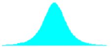 |
| 2.0 | 0.67 | 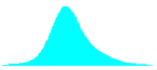 |
| 2.0 | 1.33 |  |
| 2.0 | 2.00 |  |
| 2.0 | 2.67 |  |
| 2.0 | 3.33 |  |
Table 30. Bias in estimating PD when two populations are combined (sample size = 5, 10,000 simulated lots).
| Std. Dev. Ratio | Weighted Mean Offset |
Actual PD | Bias* | 95% CI |
|---|---|---|---|---|
| One-Sided Specification Limits | ||||
| 1.0 | 0.00 | 9.99 | 0.11 | 0.22 |
| 1.00 | 9.99 | -0.07 | 0.22 | |
| 2.00 | 9.99 | -0.07 | 0.21 | |
| 3.00 | 10.00 | 0.24 | 0.20 | |
| 4.00 | 9.99 | 1.02 | 0.19 | |
| 5.00 | 9.99 | 1.80 | 0.19 | |
| 1.5 | 0.00 | 10.00 | 0.13 | 0.23 |
| 0.80 | 10.00 | 0.56 | 0.22 | |
| 1.60 | 10.00 | 1.08 | 0.20 | |
| 2.40 | 10.00 | 1.37 | 0.20 | |
| 3.20 | 10.00 | 1.93 | 0.19 | |
| 4.00 | 10.00 | 2.53 | 0.02 | |
| 2.0 | 0.00 | 10.00 | 0.98 | 0.24 |
| 0.67 | 10.00 | 1.50 | 0.23 | |
| 1.33 | 9.99 | 2.14 | 0.21 | |
| 2.00 | 10.00 | 2.37 | 0.20 | |
| 2.67 | 9.99 | 2.72 | 0.19 | |
| 3.33 | 10.00 | 3.13 | 0.19 | |
| Two-Sided Specification Limits-Equidistant From the Mean | ||||
| 1.0 | 0.00 | 10.00 | 0.05 | 0.22 |
| 1.00 | 10.00 | -0.02 | 0.21 | |
| 2.00 | 9.99 | 0.56 | 0.20 | |
| 3.00 | 9.99 | 2.27 | 0.20 | |
| 4.00 | 9.99 | 4.61 | 0.19 | |
| 5.00 | 9.99 | 6.95 | 0.18 | |
| 1.5 | 0.00 | 9.99 | -0.11 | 0.22 |
| 0.80 | 10.00 | 0.07 | 0.22 | |
| 1.60 | 10.00 | 0.57 | 0.22 | |
| 2.40 | 10.00 | 1.42 | 0.21 | |
| 3.20 | 10.00 | 2.94 | 0.20 | |
| 4.00 | 10.00 | 4.70 | 0.19 | |
| 2.0 | 0.00 | 10.00 | -0.37 | 0.24 |
| 0.67 | 10.00 | -0.25 | 0.24 | |
| 1.33 | 10.00 | 0.54 | 0.23 | |
| 2.00 | 10.00 | 1.16 | 0.23 | |
| 2.67 | 10.00 | 2.26 | 0.22 | |
| 3.33 | 10.00 | 3.44 | 0.22 | |
*Bias values that are NOT significantly different from zero are bolded.
Table 30. Bias in estimating PD when two populations are combined (sample size = 5, 10,000 simulated lots) (continued).
| Std. Dev. Ratio | Weighted Mean Offset |
Actual PD | Bias* | 95% CI |
|---|---|---|---|---|
| Two-Sided Specification Limits-5 PD in Each Tail | ||||
| 1.0 | 0.00 | 10.00 | 0.05 | 0.22 |
| 1.00 | 10.00 | -0.02 | 0.21 | |
| 2.00 | 9.99 | 0.56 | 0.20 | |
| 3.00 | 9.99 | 2.27 | 0.20 | |
| 4.00 | 9.99 | 4.61 | 0.19 | |
| 5.00 | 9.99 | 6.95 | 0.18 | |
| 1.5 | 0.00 | 9.99 | 0.16 | 0.23 |
| 0.80 | 10.00 | 0.30 | 0.22 | |
| 1.60 | 10.00 | 0.75 | 0.21 | |
| 2.40 | 10.00 | 1.79 | 0.20 | |
| 3.20 | 10.00 | 3.23 | 0.20 | |
| 4.00 | 10.01 | 5.04 | 0.19 | |
| 2.0 | 0.00 | 10.00 | -0.32 | 0.24 |
| 0.67 | 10.00 | 0.41 | 0.23 | |
| 1.33 | 10.00 | 1.14 | 0.22 | |
| 2.00 | 10.00 | 2.16 | 0.21 | |
| 2.67 | 10.00 | 2.97 | 0.20 | |
| 3.33 | 10.01 | 4.48 | 0.20 | |
*Bias values that are NOT significantly different from zero are bolded.
No AAD evaluation was conducted for bimodal distributions. The results from the PD/PWL evaluation presented above indicated that for the types of mean and standard deviation differences between populations that are likely to be combined in typical materials and construction operations, the result would be either approximately normal or unimodal skewed distributions. Since the previous AAD analyses presented above in this chapter had already evaluated the AAD bias with respect to normal and skewed distributions, it was decided that no additional AAD evaluation was necessary.
Both the PWL (and PD) estimators and the AAD estimators provided estimates with relatively little bias for the departures from normality that are likely to be encountered. Neither was obviously better or worse than the other. Based on the non-normality analysis, there is no reason to eliminate either of these quality measures, nor is there a compelling reason to select one over the other. It was decided to continue investigating both PWL and AAD as possible quality measures for use when developing payment relationships.