Achieving A High Level of Smoothness in Concrete Pavements Without Sacrificing Long-Term Performance

CHAPTER 6. SHORT-TERM CHANGES IN INITIAL SMOOTHNESS OF CONCRETE PAVEMENTS

INTRODUCTION

All SHAs that construct PCC pavements have a smoothness specification. Some smoothness specifications will give a timeframe after construction within which smoothness measurements must be performed while others do not. An issue with PCC pavements is the effect of curling and warping of PCC slabs on smoothness. Some contractors perform smoothness measurements as soon as possible after construction because they perceive that curling and warping effects on the pavement will be negligible immediately after construction. However, if curling and warping occurs in the pavement during its early life, causing a significant reduction in smoothness, the validity of bonuses paid based on smoothness measurements obtained immediately after construction becomes questionable.

A study was performed to investigate how the smoothness of a PCC pavement changes during the first 3 months of its life. Test sections were established at the following paving projects for this study:

• State Route (S.R.) 6220, Centre County, PA.
• U.S. Route 20 (U.S. 20), Hardin County, IA.
• Interstate 80 (I-80), Pottawattamie County, IA.
• U.S. Route 23 (U.S. 23), Monroe County, MI.
• Interstate 69 (I-69), Calhoun County, MI.

All of these pavements were doweled JPC pavements. The smoothness measurements were generally performed at the following time periods using an inertial profiler:

• 1 day after paving.
• 3 days after paving.
• 1 week after paving.
• 3 months after paving.

Smoothness measurements were performed in each wheel path, and three repeat measurements were performed for each data set. At several test sections, measurements were obtained in the morning and the afternoon during the 1-week and 3-month testing. At one test section, measurements were also obtained approximately 1 year after construction.

The following analyses were performed on the collected profile data:

1. Obtain average IRI and RN: Compute IRI and RN for all profile runs. Then compute an average IRI and RN for each data set using the values obtained for the three repeat runs.
2. Investigate the repeatability of the profiler: The IRI values obtained for the entire test section from the repeat runs for each data set were evaluated to determine the repeatability of the profiler.
3. Investigate the short-interval IRI repeatability: This investigation was performed by comparing IRI values at 15-m (49-ft) intervals for the repeat runs in each data set. This investigation indicates whether the distribution of the roughness within the section for the three repeat runs was repeatable. In some cases, IRI from the repeat runs for a pavement section can be very close to each other; however, the distribution of roughness within the section for the repeat runs can be variable. When the overall roughness for the section is computed, the roughness variability within the section can cancel out, and give close IRI values for repeat runs even though they may have very different roughness distributions within a section.
4. Evaluate changes in IRI and RN: Compare IRI and RN obtained the first time the section was profiled with values obtained from subsequent profiling. This analysis provides information on how the smoothness of PCC pavements changes during the first few months of their life relative to the smoothness obtained immediately after paving.
5. Evaluate the effect of joints on profile data and smoothness indices: In the two projects in Iowa, a sawcut that is 6 mm (0.25 inches) wide and 25 mm (1 inch) deep is made on the pavement. Thereafter, the joint is sealed. Profile data collected for these two conditions of the joint were available for the two Iowa projects. In the Michigan and the Pennsylvania projects, a 3-mm (0.12-inch)-wide initial sawcut is made on the pavement. Thereafter, the joint is widened to form a reservoir and then sealed. Profile data collected for all three conditions of the joint were available. These profile data were analyzed to see how the joint appeared in the profile data and to investigate the impact of these different joint conditions on IRI and RN.
6. Use roughness profiles to investigate the distribution of roughness: For this analysis, IRI roughness profiles based on an 8-m (26-ft) base length were used. Roughness profiles for the left wheel path, right wheel path, and an overlaid plot that showed profiles for both wheel paths were used in this analysis.
7. Evaluate profile characteristics: Profile data collected at different time periods were analyzed using profile plots and PSD plots to investigate changes in profile, and to see whether a dominant wavelength or a dominant waveband that is affecting IRI is present in the profile. The CI values of the profiles also were computed to investigate slab curvature.
8. CTE values and microscopical examination: Cores obtained from the pavement or cylinders cast from concrete used in the project were used to determine the CTE of the concrete and to perform a microscopical examination to identify the coarse and the fine aggregate in the concrete. The CTE test was carried out using the test procedure CRD-C 39-81 that is described in the U.S. Army Corps of Engineers Materials Testing Handbook⁽³⁶⁾. The microscopical examination of the concrete cylinder or core was performed in accordance with portions of ASTM C 856-02, Standard Practice for Petrographic Examination of Hardened Concrete⁽³⁷⁾.

The results obtained at each project are explained separately below.

STATE ROUTE 6220 PROJECT - PENNSYLVANIA

Project Description

This project involved new construction and was located in Centre County, PA. This roadway is a four-lane divided highway with two lanes in each direction. A 168-m (550-ft)-long test section was established for testing on the two southbound lanes. The test section was established between stations 588+00 and 582+50. (Stations are in U.S. customary units).

Pavement Details

Table 21 shows pavement details. The subgrade consisted of blasted rock mixed with fines. Table 22 provides information about the joints in the pavement.

Concrete Mix Design

Table 23 presents the mix proportions used for the concrete mix. An entrained air admixture and a water-reducing admixture were added to the concrete mix. Table 24 shows the gradation of the aggregates used in the concrete mix.

Paving Details

Table 25 shows the date and time of test section paving and other details related to the paving process. The concrete was placed using a slipform paver.

Profiling of Section

Eight sets of profile data were collected over a 3.5-month period. The pavement was first profiled 1 day after paving; the second set of profiles were collected 3 days after paving. The third and fourth sets of data were collected 1 week after paving in the morning and afternoon, respectively. The fifth and sixth sets of data were collected 1 month after paving in the morning and afternoon, respectively. The seventh and eighth sets of data were collected about 3.5 months after paving in the morning and afternoon, respectively. The profile data were collected using an ICC lightweight laser profiler. This profiler recorded data at 31-mm (1.2-inch) intervals.

Table 26 shows the dates and times when profile data collection was performed, the approximate age of the pavement at each instance, and the low, high, and mean air temperatures for each profiling day.

The 3-mm (0.12-inch)-wide initial sawcut had been made on the pavement when the profile data were collected 1 day after paving. The joint reservoirs had been formed, but the joints were not sealed when the profile data were collected in the morning of the 1-month data collection. The joints were sealed when the 1-month afternoon runs were performed. During the 3.5-month data collection, it was noted that the first 5.5 m (18 ft) of the inside lane had been diamond ground.

N/A: Profile data not collected

Roughness Indices

IRI Values

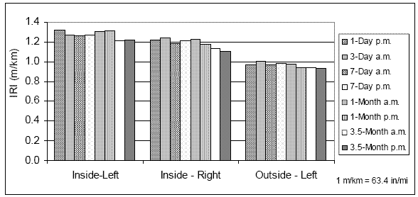
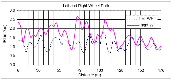
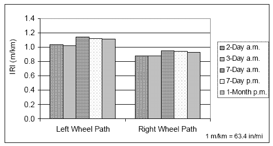
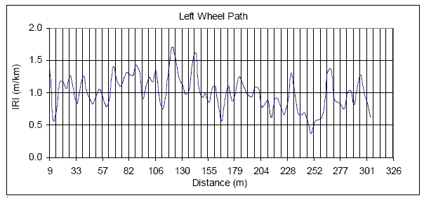
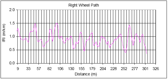
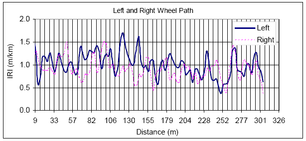
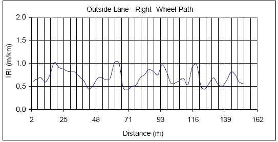
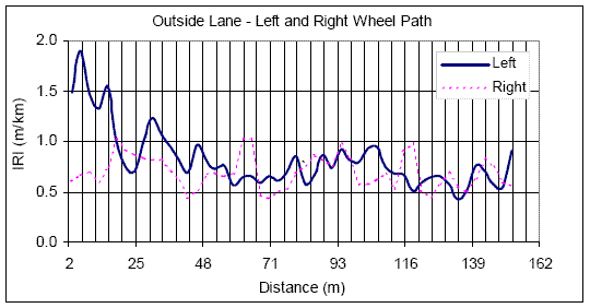
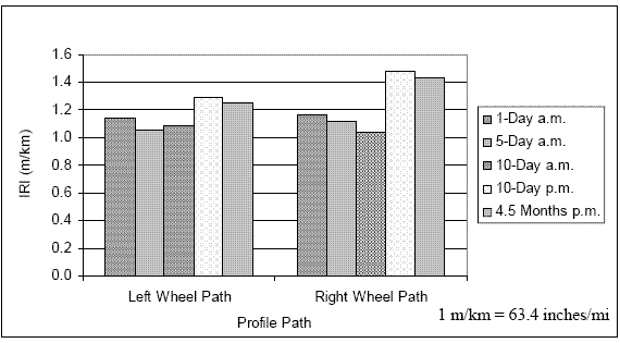
The average IRI values computed from the three repeat runs are presented in table 27 and shown graphically in figure 71. The IRI for the right wheel path in the outside lane is not shown in this figure, because data were collected along this path only during the 1-month and 3.5-month data collection. Table 28 shows the percentage change in IRI values for different test sequences with respect to the IRI obtained at 1 day. Values for right wheel of outside lane are not presented in this table because profiling was performed along this path only during the 1-month and 3.5-month data collection.

N/A: Profile data not collected

1 m/km = 63.4 inches/mi

Figure 71. IRI values for different test sequences - S.R. 6220.

Note: 1-day profile data not collected along right wheel path of outside lane

The following observations were noted when evaluating the IRI values:

• The IRI is showing a decrease transversely across the pavement from the left wheel path of the inside lane to the right wheel path of the outside lane. The 1-month afternoon IRI (obtained after the joints were sealed) indicated the IRI of the left wheel path of inside lane, right wheel path of inside lane, left wheel path of outside lane, and right wheel path of outside lane to be 1.31, 1.18, 0.94, and 0.93 m/km (83, 75, 60, and 59 inches/mi), respectively. The difference in IRI between the two wheel paths of the outside lane was small.
• The IRI values obtained during the 3.5-month testing for the inside lane for both the left and the right wheel paths were lower than the IRI obtained during 1-day testing by 8 and 9 percent, respectively. This reduction in IRI is attributed to the diamond grinding that was performed on this lane.
• When the data for the case where measurements were obtained after diamond grinding were omitted, the data show the IRI along each test path has remained relatively constant for all data sets. The changes in IRI with respect to 1-day IRI were usually within ±3 percent. The age of pavement and the time of testing do not appear to have affected the IRI.
• The joints in the pavement were at three different conditions during testing: (1) initial sawcut performed on the pavement (testing at 1 day, 3 days, and 7 days), (2) joint reservoir sawed but not sealed (1-month morning testing), and (3) joints sealed (1-month afternoon and 3.5-month testing). The condition of the joint during testing had negligible impact on the IRI.

RN Values

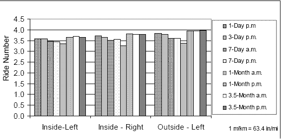
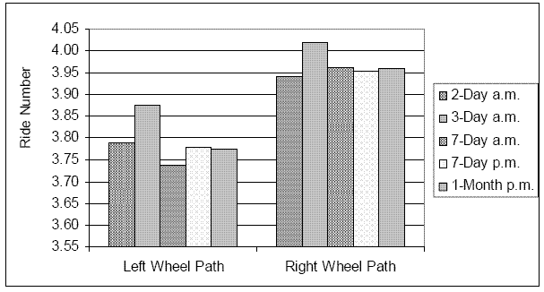
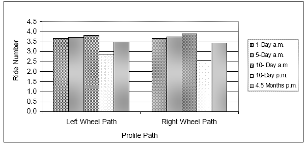
The average RN values obtained from the three runs are presented in table 29 and shown in figure 72. Table 30 shows the percentage change in RN values for different test dates with respect to the RN obtained at 1 day. The RN for the right wheel path in the outside lane is not shown in figure 72 and table 30 because data were collected along this path only during the 1-month and 3.5-month data collection.

Figure 72. RN values for different test sequences - S.R. 6220.

N/A: Profile data not collected

The following observations were noted when the RN values were evaluated:

• The RN values increased transversely across the pavement from the left wheel path of the inside lane to the left wheel path of the outside lane. The right wheel path of the outside lane had a slightly lower RN than the left wheel path of the outside lane.
• The 7-day RN values were less than the 1-day RN values; the values were lower by 4 to 6 percent for the different wheel paths. An evaluation of the profiles indicated that the backer rods put into the joints appear to have settled when 7-day profiling was performed, and this feature was appearing in the profile as a slight depression and causing lower RN values.
• The 1-month morning profiles had the lowest RN value; the RN was lower than the 1-day value by 6 to 12 percent for the different wheel paths. The joint reservoirs had been sawed when the data were collected, which caused depressions to be recorded in the profile data at the joint locations. This phenomenon caused a reduction in the RN values.
• The RN of profiles collected during the 1-month afternoon profiling when the joints were sealed had higher values than those obtained from profiles collected in the morning when the joint reservoir had been sawed and the joint was unsealed. The afternoon RN values were higher than the morning RN values by 9 to 16 percent for the different wheel paths.
• The RN values obtained after the joints were sealed (1-month afternoon runs) were slightly higher than the RN values obtained from the 1-day profiling by values ranging from 0.09 to 0.11 (2 to 3 percent) for the different wheel paths. An evaluation of the profiles did not indicate the cause for this slight increase in RN. There may have been slurry resulting from joint sawing operations adjacent to the joint during the 1-day profiling, which may have caused lower RN values.

Repeatability of IRI Values

An evaluation of the IRI values obtained from repeat runs for each data set indicated good repeatability. Usually when the IRI from three runs were compared, the difference between the maximum and the minimum IRI was between 0.02 to 0.03 m/km (1.27 to 1.90 inches/mi).

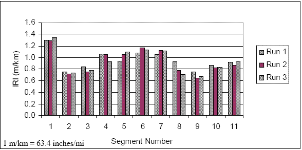
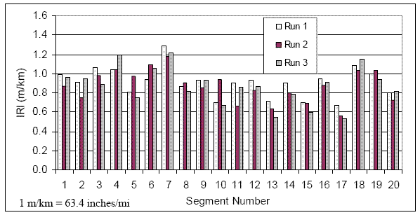
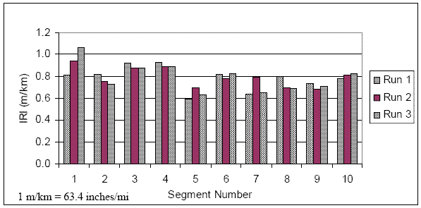
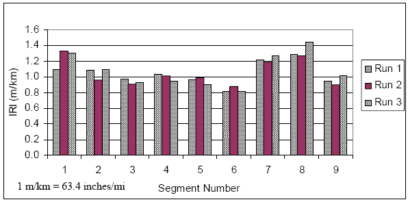
The three repeat runs obtained along the left wheel path of the outside lane for the 1-month afternoon runs were used to evaluate the short interval repeatability of IRI within the section. The IRI of each run was computed at 15-m (49-ft) intervals to perform this evaluation. The 165-m (541-ft)-long section has 11 segments that are 15 m (49 ft) long (the last 3 m (10 ft) of the section was ignored). Figure 73 shows the IRI values obtained at 15-m (49-ft) intervals for each run. Overall, reasonable repeatability in IRI values was obtained for the majority of segments. The difference between the maximum and minimum IRI for a segment obtained from the repeat runs ranged from a low of 0.03 m/km (1.9 inches/mi) at segment 2 to a high of 0.21 m/km (13.3 inches/mi) at segment 8. The average of the difference between maximum and minimum IRI for a segment was 0.09 m/km (5.7 inches/mi).

Figure 73. IRI values for repeat runs - S.R. 6220.

Effect of Condition of Joint on Profile Data

During this study, profile data were collected when the joints were in the following conditions:

• The initial sawcut that was 3 mm (0.12 inch) in width and 93 mm (3.7 inches) deep had been made on the pavement. A backer rod had been placed inside the joint. Profile data under these conditions were collected during 1-day, 3-day, and 1-week profiling.
• The joint reservoir that was 9.5 mm (0.4 inch) wide and 38 mm (1.5 inches) deep had been made on the pavement. Profile data under this condition were collected during the 1-month morning data collection.
• The joints had been sealed. Profile data under this condition were collected during the 1-month afternoon and 3.5 month data collection. According to the specification, when the joint is sealed, the depth from the pavement surface to the top of the sealant should be 5 mm (0.2 inch).

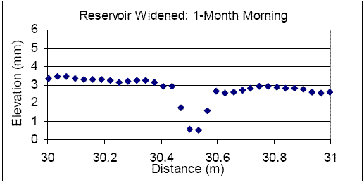
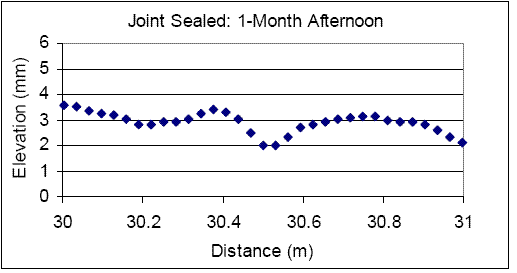
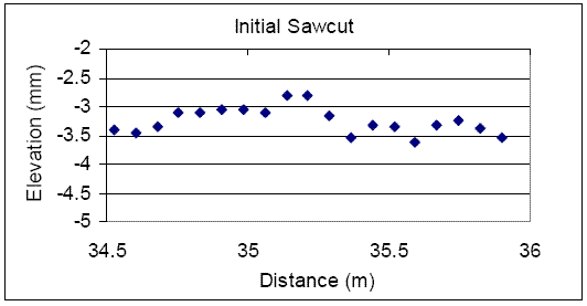
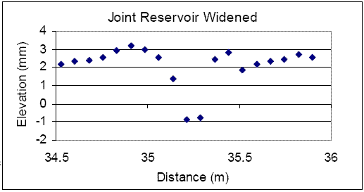
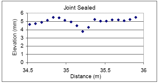
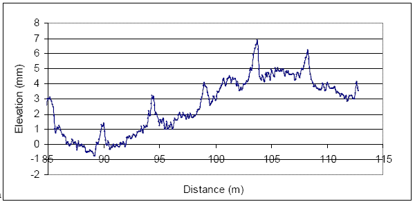
Profile data collected when the joint was at each of the three conditions described previously were evaluated to investigate how the joints showed up on the profile. Data collected along the left wheel path of the outside lane at the following profiling times were evaluated: 1 day (initial sawcut), 1-month morning (joint reservoir sawed), and 1-month afternoon (joint sealed). Figures 74 - 76 show how a typical joint appeared on the profile for each of these conditions. The joint appears between 30.4 and 30.6 m (99.7 and 100.3 ft) in the plots. The following observations are noted for each case shown in figures 74 - 76.

• Initial Sawcut: The joint appears in the profile as a small depression spread over a distance of about 220 mm (8.7 inches), with a maximum depth about of 1.5 mm (0.06 inch).
• Joint Reservoir Sawed: The joint appears in the profile as a small depression spread over a distance of about 220 mm (8.7 inches), with a maximum depth of about 3.5 mm (0.14 inch).
• Joint Sealed: The joint appears in the profile as a small depression spread over a distance of about 220 mm (8.7 inches), with a maximum depth of about 1.5 mm (0.06 inch).

For all three cases, the joint appears in the profile as a small depression spread over a distance of about 220 mm (8.7 inches), when the actual width of the joint is 9.5 mm (0.4 inch). Also, the depth of the joint that appears in the profile for each case is much less than the actual depth. This phenomenon is caused by the averaging performed on the height sensor data and the low-pass filtering that is applied on the profile data to prevent aliasing.

Figure 74. Measurements at a joint, initial sawcut, 1-day - S.R. 6220.

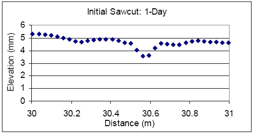
1 m = 3.28 ft
1 mm = 0.039 inch

Figure 75. Measurements at a joint, reservoir widened, 1-month morning - S.R. 6220.

1 m = 3.28 ft
1 mm = 0.039 inch

Figure 76. Measurements at a joint, joint sealed, 1-month afternoon - S.R. 6220.

1 m = 3.28 ft
1 mm = 0.039 inch

The lightweight profiler used for data collection recorded profile data at 31-mm (1.2-inch) intervals. However, the height sensor in the profiler obtains data at much closer intervals, and an averaged height sensor value is used to compute profile data points at 31-mm (1.2-inch) intervals. In addition, a low-pass filter appears to have been applied on the data further attenuating the depth of the joint, and causing the joint to appear as a much wider feature. Although the profiles obtained when the joint reservoirs had been sawed do show a downward feature at the joint that has a higher depth compared to the other two cases, the depth of the features is not large enough to have an effect on the IRI. Hence, the IRI values computed from profiles collected under the three different scenarios were very close to each other. However, the downward spikes of the magnitude seen for 1-month morning profiling where the joint reservoirs had been sawn do have a significant impact on RN. The 1-month afternoon RN values obtained after the joints were sealed were higher than the morning values by 9 to 16 percent for the different wheel paths.

Roughness Profiles

Figures 77 - 79 and figures 80 - 82 show the roughness profiles for a 6-m (20-ft) base length for the outside lane and inside lane, respectively. The roughness profile for the outside lane was computed from data obtained for the 3-month afternoon testing, whereas the roughness profile for the inside lane was computed using data obtained from 3-day testing. The joint spacing of the pavement is 4.6 m (15 ft) and each vertical line in the plots corresponds to a joint. The peaks in the plots indicate areas of high roughness. Many peaks are coinciding with the joint locations or are very close to joint locations. This situation indicates that the dowel baskets may be affecting roughness.

Figure 83 shows a high roughness area along the left wheel path of the inside lane at the start of the section. This area was subsequently diamond ground. Several localized areas of high roughness are noted along the left wheel path of the inside lane, and the roughness of these areas contributed to making this wheel path have the highest roughness of all tested wheel paths.

Evaluation of Profile Data

Apart from the differences in joint conditions, no significant differences between the profiles obtained during the different test sequences could be observed. The profiles obtained along the inside lane during 3.5 months of testing showed the effect of diamond grinding at the start of the section. Also, no distinct profile feature or a dominant waveband could be identified in the profile data.

As described previously, the IRI varied transversely across the section. The difference in IRI between the left wheel path of the inside lane and the right wheel path of the outside lane based on 1-month afternoon testing was 0.38 m/km (24 inches/mi). Evaluation of the profile data did not show a distinct profile feature that was responsible for this difference in IRI.

The CI value was computed for one profile run from each data set, and the computed values are shown in table 31. This table does not show values for the right wheel path of the outside lane because profile data were only collected along this path during the 1-month and 3.5-month data collection. The CI values for all data sets were extremely small, which indicates the slabs are more or less flat with virtually no curvature. No noticeable changes in curvature were observed between the data sets.

Figure 77. Roughness profiles for outside lane, left wheel path - S.R. 6220.

1 m = 3.28 ft
1 m/km =63.4 inches/mi

Figure 78. Roughness profiles for outside lane, right wheel path - S.R. 6220

1 m = 3.28 ft
1 m/km =63.4 inches/mi

Figure 79. Roughness profiles for outside lane, left and right wheel path - S.R. 6220.

1 m = 3.28 ft
1 m/km =63.4 inches/mi

Figure 80. Roughness profiles for inside lane, left wheel path - S.R. 6220.

1 m = 3.28 ft
1 m/km =63.4 inches/mi

Figure 81. Roughness profiles for inside lane, right wheel path - S.R. 6220.

1 m = 3.28 ft
1 m/km =63.4 inches/mi

Figure 82. Roughness profiles for inside lane, left and right wheel path - S.R. 6220.

1 m = 3.28 ft
1 m/km =63.4 inches/mi

1/m = 1/3.28 ft

Coefficient of Thermal Expansion and Microscopical Examination

A CTE test and a microscopical examination were performed on a 150-by-300 mm (5.9-by-11.8 inch) cylinder that was cast from the concrete used in the project. The CTE value for the specimen was 9.60 x 10^-6 per ^oC (5.33 x 10^-6 per ^oF). The microscopical examination identified the coarse aggregate to be primarily dolomite/dolomitic limestone (carbonate) with traces of granite (silicious). The fine aggregate was classified as silicious.

Summary

• The IRI of the pavement was decreasing transversely from the left wheel path of the inside lane to the left wheel path of the outside lane. Along the outside lane, the left and right wheel path IRI values were close to each other. The 1-month afternoon testing indicated that the IRI of the left wheel path of inside lane, right wheel path of inside lane, left wheel path of outside lane, and right wheel path of outside lane were 1.31, 1.18, 0.94, and 0.93 m/km (83, 75, 60, and 59 inches/mi), respectively. No distinct profile feature that had this effect on the IRI could be identified.
• Researchers noted that the data collected by the lightweight profiler did not accurately record the shape of the joints in the pavement. A joint appeared in the profile as a small depression spread over a distance of 220 mm (8.7 inches), when the actual width of the joint was 9.5 mm (0.37 inch). The depth of this depression varied depending on the condition of the joint. When the initial sawcut that was 3 mm (0.12 inch) wide was present, a depth of 1.5 mm (0.06 inch) was recorded. When the joint reservoir that was 9.5 mm (0.37 inch) wide and 38 mm (1.50 inches) deep was present with the joint being unsealed, a depth of 3.5 mm (0.14 inch) was recorded. When the joint was sealed, a depth of 1.5 mm (0.06 inch) was recorded.
• The profiler showed good repeatability in obtaining IRI values. When the IRI obtained from the three repeat runs for the entire section were evaluated for all data sets, the difference between the maximum and minimum IRI was between 0.02 m/km (2.5 inches/mi) and 0.03 m/km (1.9 inches/mi).
• An evaluation of short interval IRI repeatability using 15-m (49-ft) segment lengths indicated that the profiler was providing reasonable repeatability. The average difference between the maximum and minimum IRI obtained for a 15-m (49-ft)-long segment was 0.09 m/km (5.7 inches/mi).
• Little change in IRI was noted for the different data sets. The IRI can be considered to have remained at the same value over the 3.5-month period. The IRI was not affected by the condition of the joint or the time of day when profiling was performed. The IRI was not affected by the condition of the joint because the data collected by the profiler was attenuating the depth of the joint, and the recorded depths were of such a magnitude that they did not affect the IRI.
• As for the IRI, little change in RN was noted for the different data sets, except for the values obtained when the joint reservoirs had been sawed and the joint was in an unsealed condition. The RN obtained after the joint was sealed was higher than the RN obtained when the joint reservoir was formed but unsealed by 9 to 16 percent for the different wheel paths.
• There was negligible curvature in the PCC slabs for the different data sets. The slabs in the pavement can be considered to be flat. No appreciable changes in curvature were noted between the different data sets.

U.S. 20 PROJECT IN IOWA

Project Description

This was a reconstruction project located in Hardin County, IA. This roadway is a four-lane divided highway with two lanes in each direction. A 183-m (600-ft)-long test section was established for testing on the westbound inside lane. The test section was established between stations 1269+00 and 1275+00. (Stations are in U.S. customary units.)

Pavement Details

Table 32 presents pavement details. Table 33 presents information about the joints in the pavement.

Concrete Mix Design

Table 34 presents the mix proportions used in the concrete mix. An entrained air admixture and a water-reducing admixture were added to the concrete mix. Table 35 presents the gradation of the aggregates used in the concrete mix.

Paving Details

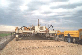
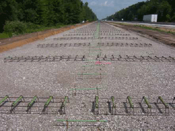
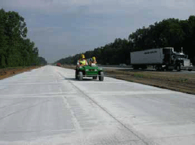
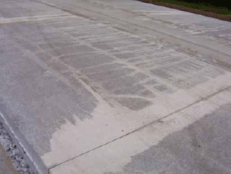
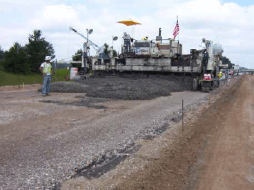
Table 36 presents the date and time when the test section was paved as well as other details about the paving process. The concrete was placed using a slipform paver. Figure 83 is a photograph of the paving operation. The paver had a super-smoother finishing attachment at the back of the paver for finishing the concrete. More than 25 mm (1 inch) of rain occurred after 8 p.m. on the day paving took place.

Profiling of Section

Six sets of profile data were collected over a 3-month period. The pavement was first profiled 1 day after paving, and then the second set of profiles was collected 3 days after paving. The third and fourth sets of data were collected approximately 1 week after paving in the morning and afternoon, respectively. The fifth and sixth sets of data were collected 3 months after paving in the morning and afternoon, respectively, of the same day. The profile data collection was performed using an Ames lightweight profiler that recorded data at 30-mm (1.2-inch) intervals. Table 37 shows the dates and times when profile data collection was performed, the approximate age of the pavement at each of these instances, and the low, high, and mean air temperatures for each profiling day.

A 6-mm (0.25-inch)-wide and 25-mm (1-inch)-deep sawcut had been made on the pavement when the profile data were collected for the first time. The joints were sealed after the 3-day data collection was performed.

Figure 83. Paver in operation.

Roughness Indices

IRI Values

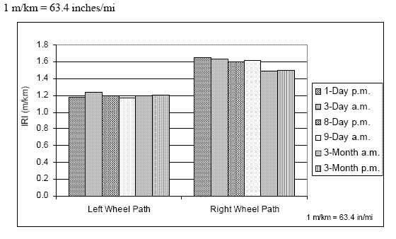
The average IRI values computed from the three repeat runs are presented in table 38 and shown in figure 84. Table 39 shows the percentage change in IRI values for different test sequences with respect to the IRI obtained at 1 day.

Note: Joints were sealed after the 3-day data collection
1 m/km = 63.4 inches/mi

Figure 84. IRI values for different test sequences - U.S. 20.

The following observations were noted when evaluating the IRI values:

• The IRI of the right wheel path was higher than the left wheel path for all test sequences. For the different test sequences, IRI of the right wheel path was higher than that for the left wheel path by amounts ranging from 24 to 40 percent. The highest difference was observed for the testing that was performed 1 day after paving.
• Overall, the IRI remained relatively constant along the left wheel path for all test dates and times. The percentage difference in IRI with respect to the 1-day IRI for the different test sequences ranged from -1 to 5 percent. Along the right wheel path, the percentage difference in IRI with respect to the 1-day IRI for testing performed within the first 9 days ranged from -1 to -3 percent. However, the IRI obtained at 3-month testing was approximately 10 percent lower than that obtained for 1-day testing. The cause for this reduction could not be identified by evaluating the profile data.
• The joints were sealed after the 3-day profiles were obtained. The 1-week IRI values did show a reduction in IRI of 0.04 m/km (2.5 inches/mi) compared to the 3-day IRI value. However, this reduction is extremely small and indicates that similar IRI values were obtained when the joints were unsealed and sealed.

RN Values

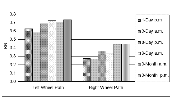
The average RN obtained from the three repeat runs are presented in table 40 and shown in figure 85. Table 41 shows the percentage change in RN values for different test sequences with respect to RN obtained at 1 day. The following observations were noted when evaluating the RN values:

• The RN of the left wheel path was higher than that for the right wheel path for all test sequences; the difference in RN ranged from 7 to 10 percent.
• Overall, RN remained relatively constant along both wheel paths for all test sequences. Along the left wheel path, the difference in RN for different test sequences compared to 1-day RN ranged from -1 to 3 percent. This difference for the right wheel ranged from 0 to 5 percent; the highest difference observed was for testing performed at 3 months.
• The joints were sealed after the 3-day profiles were obtained. The 1-week RN values showed an increase in RN of about 0.10 from the 3-day values. This level of increase shows that sealing the joints had a very small effect on RN.

Note: Joints were sealed after the 3-day data collection

Figure 85. RN values for different test sequences to U.S. 20.

Repeatability of IRI Values

On average, when all data sets were considered, the difference between the maximum and minimum IRI values obtained from the three repeat runs was 0.06 m/km (3.8 inches/mi).

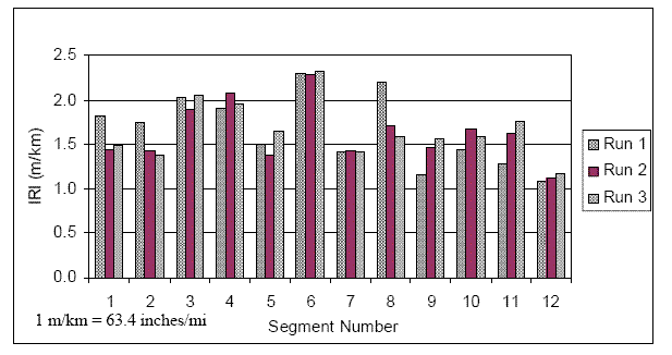
The three repeat runs collected along the left wheel path for day-1 testing were used to evaluate the short interval IRI repeatability by comparing IRI values obtained at 15-m (49-ft) intervals. For the 183-m (600-ft)-long section, there are twelve 15-m (49-ft) long segments (the last 3 m (10 ft) of the section was ignored). Figure 86 shows the IRI values obtained at 15-m (49-ft) intervals for the three runs.

An evaluation of the IRI values shown in figure 86 indicates that the IRI values from the different runs were variable for many segments. The difference between the maximum and minimum IRI for each segment obtained from the three repeat runs ranged from a low of 0.02 m/km (2.5 inches/mi) that occurred at segment 6, to a high of 0.60 m/km (38 inches/mi) that occurred at segment 8. The average of the difference between maximum and minimum IRI from the three runs when all segments were considered was 0.25 m/km (16 inches/mi).

The IRI for the entire section obtained from the three repeat runs were very close to each other; the IRI values were 1.66, 1.64, and 1.66 m/km (105, 104, and 105 inches/mi). Although the IRI values for the whole section from the three repeat runs were very close to each other, the distribution of the IRI within the section was very different for the three runs. When the overall IRI for the section is computed, the variations of the IRI within the section for a run are averaged out.

Figure 86. IRI values for repeat runs - U.S. 20.

This pavement section has longitudinal tining. When profile data are collected at this type of section, because of lateral variations in the profile path, the laser dot of the height sensor in the profiler can sometimes traverse along the top of the tining and sometimes dip into the tining and collect data at the bottom of the tining. This phenomenon can result in very different data being collected for repeat runs. The high variability in IRI values between the runs when IRI of 15-m (49-ft) segments were considered is attributed to this phenomenon.

Effect of Joint Condition on Profile Data

The joints were not sealed when the 1-day and 3-day profile data collection was performed. The joints were sealed immediately after the 3-day data collection. Profiles obtained before and after joint sealing were evaluated to investigate how the joints appear on the profile. The left wheel path data collected at 1-day and 1-month afternoon were used in this evaluation.

Figures 87 - 88 show how a typical unsealed and a sealed joint appeared in the profile data. The joint is approximately at a distance of 48 m (157 ft) in the plots. The joint reservoir is 6 mm (0.25 inch) wide. In the unsealed condition, the joint depth was 25 mm (1 inch). When the joint was sealed, the depth to the top of the sealant from the pavement surface was approximately 6 mm (0.25 inch). Although the joint is 6 mm (0.25 inch) wide, the joint appears in the profile as a feature spread over a distance of approximately 300 mm (11.8 inches). The profile plots indicated a depth at a joint of about 2 mm (0.08 inches) and 1 mm (0.04 inches) for the unsealed and sealed condition, respectively.

Figure 87. Measurements at a joint, unsealed - U.S. 20.

Figure 88. Measurements at a joint, sealed - U.S. 20.

As described previously when discussing joint conditions for the S.R. 6220 project, averaging effects of the height sensor and the anti-alias filter applied on the profile data causes the joint depth to be attenuated as well as the joint to appear as a feature spread over a distance much wider than the actual width of the joint. There is a small difference (approximately 1 mm (0.04 inch)) in the magnitude of the depth of the dip between the unsealed and sealed conditions. However, this difference in magnitude has no effect on IRI; hence, no difference in IRI between the sealed and the unsealed conditions was observed. However, this feature does appear to have a small impact on RN; the RN value increased by 0.1 after the joints were sealed.

Roughness Profiles

The IRI roughness profiles for a 6-m (20-ft) base length for the left wheel path, right wheel path, and an overlaid plot of the two wheel paths obtained from data collected during day-1 testing is shown in figures 89 - 91. The vertical lines in the plots correspond to joint locations.

The roughness profiles show that the roughness of the right wheel path is much higher than that for the left wheel path up to a distance of 128 m (420 ft), but after that the roughness levels of the two wheel paths are close to each other. Some peaks in the roughness profiles, particularly after a distance of 128 m (420 ft) correspond to or are very close to a joint. This phenomenon may indicate a possible effect of dowel baskets on roughness level.

Figure 89. Roughness profiles for U.S. 20, left wheel path.

1 m = 3.28 ft
1 m/km = 63.4 inches/mi

Figure 90. Roughness profiles for U.S. 20, right wheel path.

1 m = 3.28 ft
1 m/km = 63.4 inches/mi

Figure 91. Roughness profiles for U.S. 20, left and right wheel path.

1 m = 3.28 ft
1 m/km = 63.4 inches/mi

Evaluation of Profile Data

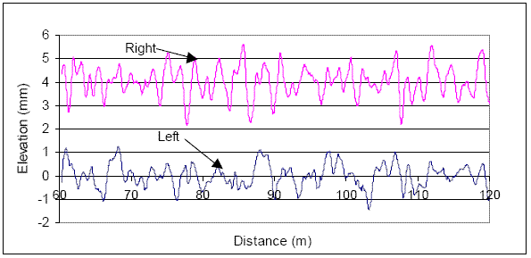
An evaluation of the profile data indicated the presence of a repetitive wave in the right wheel path that had an approximate wavelength of 1.6 m (5.2 ft). This wave was not observed in the left wheel path profile. Figure 92 shows a band-pass filtered profile plot of the data collected along the left and the right wheel paths, with the profiles offset for clarity. The right wheel path shows more waviness, which is caused by the repetitive wave.

Figure 92. Band-pass filtered elevation profile.

1 m = 3.28 ft
1 mm = 0.039 inch

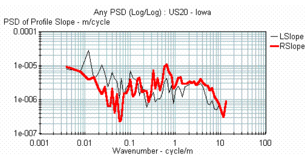
Figure 93 shows the PSD plot of the left and right wheel path data. The right wheel path profile shows higher roughness between wavenumbers of 0.29 and 2.05 m/cycle (0.95 and 6.7 ft/cycle) compared to the left wheel path. These wavenumbers correspond to wavelengths between 0.5 and 3.5 m (11.5 ft). The cause for the high IRI of the right wheel path compared to the left wheel path is attributed to the higher roughness contribution between these wavelengths. The right wheel path PSD plots shows a peak at wavenumber of 0.65 cycles/m (2.1 cycle/ft), which corresponds to a wavelength of 1.6 m (5.2 ft). This is the dominant repetitive wavelength seen in the right wheel path profile.

The CI value was computed for one profile run from each data set. The computed values are shown in table 42. The CI values obtained for this project were somewhat higher than CI values obtained for the other projects. Some changes in CI were also noted between the data sets. The CI is influenced not only by slab curling that affects the slab over the 6-m (20-ft) slab length, but also other curvature within the slab. For example, for this pavement, the repetitive wave that has a wavelength of 1.6 m (5.2 ft) has a significant effect on CI. Evaluation of the profile data did not indicate much movement in the slabs at the joints for the different data sets. However, changes in slab shapes occurring in other areas between the different data sets contributed to changes in CI between the data sets. Generally, CI for data collected in the afternoon had higher CI values; these values were negative, which indicate downward curvature.

Figure 93. PSD plots of profiles.

1 m = 3.28 ft

1/m = 1/3.28 ft

Coefficient of Thermal Expansion and Microscopical Examination

A CTE test conducted on a 100-by-275-mm (4-by-10.8-inch) core indicated a value of 9.83 x 10^-6 per ^oC (5.46 x 10^-6 per ^oF.) A microscopical examination indicated that the coarse aggregate was limestone (carbonate) and the fine aggregate was silicious.

Summary

• The IRI of the right wheel path was significantly higher than the left wheel path. The right wheel path IRI at 1 day was 1.65 m/km (105 inches/mi), which was 40 percent higher than that of the left wheel path.
• The profile data indicated that the right wheel path had higher roughness between wavelengths of 0.5 and 3.5 m (11.5 ft) compared to the left wheel path. An evaluation of the profile data indicated that a repetitive wave having a wavelength of approximately 1.6 m (5.2 ft) was present on the right wheel path; this wave was a primary contributor to the high IRI observed along the right wheel path. This phenomenon was not observed in the left wheel path data. The factor in the paving process that caused this feature to appear in the right wheel path profile could not be identified. The paver had a super smoother float attached to the back. It is possible that the finishing procedure of this attachment may have caused this feature to appear in the profile.
• Researchers noted that the data collected by the lightweight profiler did not accurately record the shape of the joints in the pavement. In the profile, a joint appeared as a small dip that was spread over a distance of 300 mm (11.8 inches) when the actual width of the joint was 6 mm (0.25 inch). The depth of this dip was about 2 mm (0.08 inch) and 1 mm (0.04 inch) when the joint was unsealed and sealed, respectively. The actual depth of the joint was 25 mm (1 inch) in the unsealed condition. When the joint was sealed, the specification showed that the distance to the top of the sealant from the pavement surface was 6 mm (0.25 inch).
• When the IRI obtained from the three repeat runs for the entire section were evaluated for all data sets, the average of the difference between the maximum and minimum IRI was 0.06 m/km (3.8 inches/mi).
• An evaluation of short-interval IRI repeatability using 15-m (49-ft) segment lengths indicated that the IRI repeatability of the profiler was poor. The average difference between the maximum and minimum IRI obtained from the repeat runs for a 15-m (49-ft)-long segment was 0.25 m/km (16 inches/mi). The PCC pavement had longitudinal tining, and the high difference in IRI obtained between runs is attributed to the longitudinal tining. The profiler is equipped with a laser height sensor that has a diameter of about 1.5 mm (0.06 inches). Due to lateral variability, the laser can take measurements on top of the tining as well as at the bottom when traversing the section. This phenomenon can have a significant effect on the IRI. However, in comparing the IRI values obtained from repeat runs for the entire section that was 183 m (600 ft) long, they showed reasonable repeatability, because variations in IRI within the section tend to compensate when IRI is computed over longer lengths.
• Little change in IRI was noted for the different data sets along the left wheel path, and the IRI can be considered to have remained at the same value over the 3-month monitoring period. Along the right wheel path, little change in IRI was noted for data obtained up to 9 days. However, the data collected at 3 months showed a 10-percent reduction in IRI compared to that obtained 1 day after paving. The cause for this reduction could not be determined from the profile data.
• IRI obtained when the joints were unsealed and sealed were similar. The averaging and lowpass filtering performed on the profile data attenuates the depth of the joint recorded in the profile data. The depth of the joints recorded by the profiler when the joint was not sealed and sealed was 2 mm (0.08 inches) and 1 mm (0.04 inches), respectively. This difference in depth is not significant enough to have an effect on the IRI.
• A slight increase in RN was noted when RN obtained at different times were compared with the 1-day values. However, the increase in RN was less than 5 percent for all cases. The RN obtained when the joints were sealed was 0.1 higher than that obtained when the joint was not sealed.
• The CI values for this pavement were higher than that obtained for the other four projects evaluated in this study. Some changes in CI were observed between data sets that were collected at different times. It appears that the changes in CI are not being influenced by slab curling that occurs over the entire 6-m (20-ft) slab length, but by changes in other wavelengths in PCC slabs that were introduced during the construction.

I-80 PROJECT IN IOWA

Project Description

This project was a reconstruction project and is located in Pottawattamie County, IA. This roadway is a four-lane divided highway with two lanes in each direction. A 305-m (1,000-ft)- long test section was established on the eastbound outside lane.

Pavement Details

Table 43 presents details of the pavement section. The joint details of this section are similar to those for the U.S. 20 project (see table 33).

Concrete Mix Design

Table 44 presents the mix proportions used in the concrete mix. An entrained air admixture and a water-reducing admixture were added to the concrete mix. Table 45 presents the gradation of the aggregates used in the concrete mix.

Paving Details

Table 46 presents the date and time the test section was paved and other details regarding the paving process. The concrete was placed using a slipform paver. Two photographs of the paving process are shown in figures 94 and 95.

Profiling of Section

Five sets of profile data were collected over a 1-month period. The pavement was first profiled 2 days after paving, and the second set of profiles was collected 3 days after paving. The third and fourth sets of data were collected 1 week after paving in the morning and afternoon, respectively. The fifth set of data was collected 1 month after paving in the afternoon. The profile data collection was performed using an Ames lightweight profiler.

Figure 94. Overall view of the paving train.

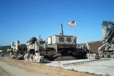
Figure 95. Slipform paver used for paving..

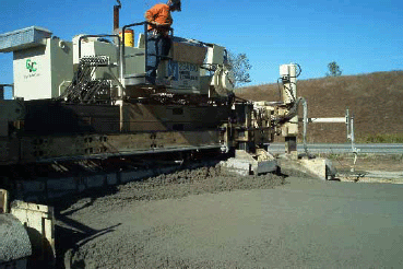
Table 47 shows the dates and times when profile data collection was performed, the approximate age of the pavement at each of these instances, and the low, high, and mean air temperatures for each profiling day.

The joints had been sealed except for the first 76 m (249 ft) of the test section when the 2-day testing was performed.

Roughness Indices

IRI Values

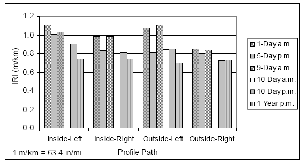
The IRI was computed for the entire 304.8-m (1,000-ft)-long test section as well as for each of the two 152.4-m (500-ft)-long sections contained within the section. The average IRI values (computed using values obtained from three runs) are shown in table 48. The IRI values for the 304.8-m (1,000-ft)-long section for the different test sequences are shown in figure 96. Table 49 shows the percentage change in IRI values for different test sequences with respect to IRI obtained from 2-day testing.

Note: Joints were not sealed in the first 76 m (249 ft) of the section during 2-day profiling. Joints were sealed for all other profiling days.

1 m/km = 63.4 inches/mi

Figure 96. IRI values for different test sequences for entire test section - I-80.

The following observations were noted when evaluating the IRI values:

• When the entire 304.8-m (1,000-ft) section was considered, the IRI of the left wheel path was higher than the right wheel path by 16 to 21 percent for the different test sequences.
• When the individual 152.4-m (500-ft)-long sections were considered, very little difference in the IRI was noted between the 2-day and 3-day testing. However, when the 7-day and 1- month IRI values were evaluated, these values were higher than the values obtained from 2- day testing by amounts ranging from 2 to 14 percent for the different test dates and wheel paths. For the first 152.4 m (500-ft) section, the IRI at 1 month was 13 percent and 2 percent higher than the 2-day testing for left and right wheel paths, respectively. For the second 152.4 m (500-ft) section, the IRI at 1 month was 3 percent and 10 percent higher than the 2-day testing for left and right wheel paths, respectively.

RN Values

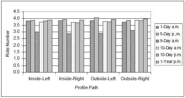
RN was computed for the entire 304.8-m (1,000-ft)-long section, as well as for the two 152.4-m (500-ft)-long sections contained within it. The average RN values are tabulated in table 50. The RN values for the 304.8-m (1,000-ft)-long section for the different test dates and times are shown in figure 97. Table 51 shows the percentage change in RN for different test sequences with respect to RN obtained from 2-day testing.

Note: Joints were not sealed in the first 76 m (249 ft) of the section during 2-day profiling. Joints were sealed for all other profiling days.

Figure 97. RN values for different test sequences for entire test section - I-80.

The following observations were noted when evaluating the RN values:

• When the entire 304.8-m (1,000-ft) section was considered, the RN of the right wheel path was higher than that for the left wheel path by amounts ranging by 4 to 6 percent for the different test sequences.
• When the first 152.4-m (500-ft) section was considered, the RN of the two wheel paths changed by amounts varying from -1 to 3 percent from the 2-day RN for the different test sequences. When the second 152.4-m (500-ft) section was considered, the RN of the two wheel paths changed by amounts varying by -3 to 1 percent from the 2-day RN for the different test sequences. These changes are negligible, and for all practical purposes, the RN can be considered to have remained constant for all test sequences.

Repeatability of IRI Values

When all profile data sets were considered, the average difference between the maximum and minimum IRI values from the three repeat runs was 0.09 m/km (5.7 inches/mi) when the entire section was considered. When the two 152.4-m (500-ft) sections within the test section were considered individually, this value was 0.11 and 0.12 m/km (7.0 and 7.6 inches/mi) for the first and the second sections, respectively.

The short-interval IRI repeatability was evaluated using the data collected for 2-day testing along the right wheel path. For each run, the IRI values were computed at 15-m (49-ft) intervals to perform this evaluation. For the 304.8-m (1,000-ft)-long section, there are 20 15-m (49-ft)-long segments (the last 4.8 m (16 ft) was omitted). Figure 98 shows the IRI values that were obtained at each 15-m (49-ft)-long segment for the three runs. The IRI values for the segments obtained from the different runs showed high variability for several segments. The difference between the maximum and minimum IRI of the segments obtained from the three repeat runs ranged from a low of 0.07 m/km (4.4 inches/mi) that occurred at segment 16, to a high of 0.27 m/km (17 inches/mi) that occurred at segment 10, with an average value of 0.14 m/km (8.8 inches/mi).

Figure 98. IRI values from repeat runs - I-80.

As in the U.S. 20 project, the IRI for the entire section for the three repeat runs used in this analysis were very close to each other, with the IRI values being 0.91, 0.87, and 0.87 m/km (58, 55, and 55 inches/mi). However, the distribution of the IRI within the section was different for the three runs. The IRI variations tend to compensate for each other when data are averaged over the entire section, and this is the reason why the overall IRI for the three repeat runs were very close to each other, even though the IRI distribution within the section for the three runs showed variability.

This pavement has longitudinal tining similar to the U.S. 20 project. As described for the U.S. 20 project, the variability between runs for short interval IRI in this project is also attributed to the longitudinal tining.

Effect of Condition of Joint on Profile Data

The method used to form joints in this section was similar to that used for the test section in U.S. 20, where joints were formed using a soft cut saw that sawed a joint reservoir 6 mm (0.25 inch) wide and 25.4 mm (1 inch) deep. Profile data collection for this section was performed using the same profiler that collected data at the U.S. 20 test section. The effect of the condition of the joint (sealed versus unsealed) that was seen in the profile data at this test section was similar to the observations noted at the test section located on U.S. 20.

Roughness Profiles

Figures 99 - 101 show IRI roughness profiles based on a 6-m (20-ft) base length for day-3 testing for the left wheel path, right wheel path, and an overlaid plot of the two wheel paths.

Figure 99. Roughness profiles for I-80, left wheel path.

1 m = 3.28 ft 1 m/km = 63.4 inches/mi

Figure 100. Roughness profiles for I-80, right wheel path.

1 m = 3.28 ft 1 m/km = 63.4 inches/mi

Figure 101. Roughness profiles for I-80, left and right wheel path.

1 m = 3.28 ft 1 m/km = 63.4 inches/mi

The vertical lines in the plots correspond to joint locations. The left wheel path shows a higher roughness level than the right wheel path, particularly for the first 155 m (508 ft) of the section. Except for some localized areas, the 6-m (20-ft) base length IRI along the right wheel path was less than 1 m/km (63 inches/mi). Some peaks in the roughness profiles are coinciding with the joint or are very close to the joint, which may indicate a possible effect of dowel baskets on the roughness.

Evaluation of Profile Data

No differences could be observed in profile data for the different test sequences. In addition, no distinct profile feature or dominant waveband that had a significant influence on the roughness could be identified in the profile data.

The CI value was computed for one profile run from each data set, and the computed values are presented in table 52. These CI values are very small, which indicates that the pavement is essentially in a flat condition. No noticeable changes in curvature have occurred over the monitored period.

1/m = 1/3.28 ft

Coefficient of Thermal Expansion and Microscopical Examination

A CTE test was conducted on a 100-by-200-mm (4-by-8-inch) cylinder made from the concrete used in this project. The CTE value for the specimen was 13.2 x 10-6 per ^oC (7.33 x 10-6 per ^oF). A microscopical examination indicated that the coarse aggregate was quartzite (silicious) and the fine aggregate was silicious.

Summary

• The IRI of the left wheel path was higher than that of the right wheel path by 16 to 21 percent for the different test sequences.
• The joint dimensions in the pavement for this project were similar to that in the U.S. 20 project. Also, the same lightweight profiler was used to collect profile data. Similar observations noted for the U.S. 20 project regarding measurement of joints and impact of joints on roughness indices were noted for this project.
• When the IRI values obtained from the three repeat runs for each individual 152.4-m (500-ft)-long sections were evaluated for all data sets; the average of the difference between the maximum and minimum IRI was 0.12 m/km (7.6 inches/mi). The longitudinal tining in the sections caused this high difference to occur.
• An evaluation of short-interval IRI repeatability using 15-m (49-ft) segment lengths indicated that the IRI repeatability of the profiler was generally low. The average difference between the maximum and minimum IRI obtained from the runs for a 15-m (49-ft)-long segment was 0.14 m/km (8.9 inches/mi). The PCC pavement had longitudinal tining, and the high difference in IRI obtained between runs is attributed to the effect of longitudinal tining.
• Changes in left as well as right wheel path IRI compared to the 2-day IRI were noted for testing performed at 7 days and 1 month. The lowest changes in IRI were noted along the right wheel path of the first 152.4-m (500-ft)-long section, where the change in IRI ranged from -2 to 6 percent. The highest change in IRI was noted along the left wheel path of the second 152.4-m (500-ft)-long section, where the change in IRI ranged from -1 to 14 percent.
• The RN values for both wheel paths of the two 152.4-m (500-ft)-long sections showed little change for the different profiling dates over the 1-month period. The change in RN compared to the 2-day RN was within ±3 percent for the different profiling times over the 1-month period.
• There was negligible curvature in the PCC slabs for the different data sets. Hence, the PCC slabs can be considered to be flat. No noticeable changes in curvature were noted between the different test sequences.

U.S. 23 PROJECT IN MICHIGAN

Project Description

This project was a reconstruction project located in Monroe County, MI. This roadway is a four-lane divided highway with two lanes in each direction. A 157-m (515-ft)-long test section was established for testing on the two southbound lanes. The test section was established between stations 739+85 and 745+00. (Stations are in U.S. customary units.)

Pavement Details

Table 53 provides pavement details. Table 54 presents information about the joints in the pavement.

Concrete Mix Design

Table 55 presents the mix proportions used in the concrete mix. An air-entraining admixture and a water-reducing admixture were added to the concrete mix. Table 56 presents the gradation of the aggregates used in the concrete mix. The coarse aggregate consisted of a mix of Michigan DOT (MDOT) 4AA and 6AAA limestone aggregate.

Paving Details

Table 57 presents the date and time of paving of the test section as well as other details about the paving process. The paving commenced at 6:30 a.m. and stopped at 11:30 a.m. because rain was predicted later for that day. It started to rain in the afternoon.

Figure 102 shows the view of the base course ahead of the paver and shows the tie bars and dowel baskets placed on the base. Figure 103 shows a view of the paving train used in the project, which consisted of a spreader, slipform paver, and the curing/texturing unit.

Figure 102. Tie bars and dowel basket placed on base.

Profiling of Section

Five sets of profile data were collected at the test section in 2003 within a 10-day period. The profile data were collected using a lightweight profiler that was owned by MDOT, which was using software developed by Transology Association. Figure 104 shows a photograph of the lightweight profiler. This profiler is equipped with a laser height sensor and recorded profile data at 76-mm (3-inch) intervals.

The pavement was first profiled 1 day after paving. Initial sawcuts over joints had been completed a short time before profiling, and dry slurry from the saw-cutting operation was present adjacent to the joints. The second set of data was collected 5 days after paving. The third set of data was collected 9 days after paving in the morning. The joint reservoirs were sawed and unsealed when the profile data were collected. The contractor sealed the joints in the afternoon. The fourth and fifth sets of data were collected on the 10^thday after paving in the morning and the afternoon, respectively.

Figure 103. View of the paving train.

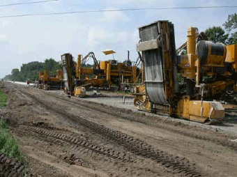
Figure 104. Profile data collection using a lightweight inertial profiler.

Approximately 1 year after paving, profile data were collected at the test section using a Dynatest high-speed profiler. This profiler is equipped with laser height sensors and recorded profile data at 25-mm (1-inch) intervals. Figure 105 shows a photograph of the Dynatest high-speed profiler.

Figure 105. High-speed inertial profiler.

Table 58 presents the dates and times when profile data collection was performed, the approximate age of the pavement at each instance, and the low, high, and mean air temperatures for each data collection date.

Roughness Indices

IRI Values

The average IRI values (computed from the three repeat runs) are presented in table 59 and shown in figure 106. Table 60 shows the percentage change in IRI values for the different test sequences with respect to the IRI obtained at 1 day.

Notes:

1. Initial sawcut 3-mm (0.12-inch)-wide present when data were collected at 1 and 5 days.
2. Joint reservoir had been sawed but unsealed when data were collected at 9 days.
3. Joints were sealed when data were collected at 10 days.

1 m/km = 63.4 inches/mi

Figure 106. IRI values for different test sequences - U.S. 23.

Notes:

1. Joint reservoir had been sawed but unsealed when data were collected at 9 days.
2. Joints were sealed when data were collected at 10 days.

The following observations were noted when evaluating the IRI values:

• The mean IRI of the inside lane was slightly higher than the IRI of the outside lane. Based on the average obtained for all test sequences, the inside lane had a mean IRI that was 9 percent higher than the IRI of the outside lane.
• For all wheel paths, the IRI obtained at 5 days was lower than the IRI obtained at 1 day, with the reduction in IRI ranging from 7 to 24 percent for the different wheel paths.
• For all wheel paths, the IRI obtained at 9 days was higher than the IRI obtained at 5 days. When the 5-day data collection was performed, the initial sawcut that was 3 mm (0.12 inch) wide had been made on the pavement. When the 9-day data collection was performed, the joint reservoirs had been sawed on the pavement, but the joints had not been sealed. The increase in IRI for the 9-day testing is attributed to these open joint reservoirs present on the pavement. The increase in IRI at 9-day data collection with respect to the 5-day data collection was 2, 18, 35, and 5 percent for the inside lane left wheel path, inside lane right wheel path, outside lane left wheel path, and outside lane right wheel path, respectively.
• For all wheel paths, the IRI obtained at 10 days was lower than the IRI obtained at 9 days. When the 9-day data collection was performed, the joint reservoirs had been sawed on the pavement, but the joints had not been sealed. The joints had been sealed when the 10-day data collection was performed. The reduction in IRI for the 10-day testing compared to the 9-day testing is attributed to the sealing of the joints. The reduction in IRI due to sealing of the joints was 13, 19, 23, and 16 percent for the inside lane left wheel path, inside lane right wheel path, outside lane left wheel path, and outside lane right wheel path, respectively.
• No appreciable changes in IRI values were noted for the morning and afternoon IRI values obtained from data collected during the 10-day profiling.
• The IRI values obtained from day-10 profiling was less than the IRI obtained from day-1 profiling by values ranging from 18 to 21 percent for the different wheel paths.
• The IRI obtained from data collected 1 year after paving was the lowest IRI obtained for all test sequences, except for the right wheel path of the outside lane. The IRI at 1 year was lower than the IRI at 1 day by 33, 25, 35, and 14 percent for the inside lane left wheel path, inside lane right wheel path, outside lane left wheel path, and outside lane right wheel path, respectively. The IRI at 1 year was lower than the IRI at 10-day by 17, 9, and 18 percent for the inside lane left wheel path, inside lane right wheel path, and outside lane left wheel path, respectively. For the outside lane right wheel path, the 1-year IRI was 1 percent higher than the 10-day IRI.
• Overall, a general reduction in IRI over time was noted.

RN Values

The average RN values are presented in table 61 and shown in figure 107. Table 62 shows the percentage change in RN values for the different test sequences with respect to the RN obtained at 1 day.

The following observations were noted when evaluating the RN values:

• A slight increase in RN was obtained for 5-day data compared to those from 1-day data. For the different wheel paths, the 5-day RN values were higher by amounts ranging from 1 to 6 percent.
• For all wheel paths, the RN obtained at 9 days was lower than the RN obtained at 1 day. When the 1-day data collection was performed, the initial sawcut that was 3-mm (0.12 inch) wide had been made on the pavement. When the 9-day data collection was performed, the joint reservoirs had been sawed on the pavement, but the joints had not been sealed. The decrease in RN for the 9-day testing is attributed to these open joint reservoirs. The RN for 9-day testing was lower than the RN from 1-day testing by amounts ranging from 17 to 25 percent for the different wheel paths.
• The 10-day RN values were very close to 1-day RN values. The difference between 10-day RN and 1-day RN ranged from -1 to 4 percent for the different wheel paths.
• The 1-year RN values were very close to 1-day RN values, but slightly higher for all cases. The difference between 1-year RN and 1-day RN ranged from 2 to 3 percent for three wheel paths; in contrast, for the right wheel path of the outside lane this difference was 7 percent.
• Overall, little difference in RN occurred over a 1-year period at this section.

Notes:

1. Initial sawcut 3 mm (0.12 inch) wide present when data were collected at 1 and 5 days.
2. Joint reservoir had been sawed but unsealed when data were collected at 9 days.
3. Joints were sealed when data were collected at 10 days.

Figure 107. RN values for different test sequences - U.S. 23..

Notes:

1. Initial sawcut 3 mm (0.12 inch) wide present when data were collected at 1 and 5 days.
2. Joint reservoir had been sawed but unsealed when data were collected at 9 days.
3. Joints were sealed when data were collected at 10 days.

Repeatability of IRI Values

When the IRI from three runs for all test sequences were evaluated, the difference between the maximum and the minimum IRI was between 0.01 to 0.11 m/km (0.6 to 7.0 inch/mi), with the average difference being 0.06 m/km (3.8 inches/mi).

An evaluation of the repeatability of short-interval IRI was performed by computing IRI at 15-m (49-ft) intervals for the three repeat runs collected along the left wheel path of the inside lane for the day-10 morning runs. For the 156-m (512-ft)-long section, there are 10 15-m (49-ft) long segments (the last 6 m (20 ft) of the section were not considered). Figure 108 shows the IRI values that were obtained at 15-m (49-ft) intervals for each run for each segment.

Figure 108. Repeatability of IRI values - U.S. 23.

A few sections had significant differences in IRI values between runs. The difference between the maximum and minimum IRI for each segment obtained from the three repeat runs ranged from a low of 0.04 m/km (2.5 inches/mi) that occurred at segment 4, to a high of 0.25 m/km (15.6 inches/mi) that occurred at segment 1, with an average 0.10 m/km (6.3 inches/mi). The IRI values obtained from the three runs for the entire section were 0.79, 0.80, and 0.79 m/km (50, 51, and 50 inches/mi). Significant differences in IRI were shown for repeat runs at a few 15-m (49-ft) segments. However, when IRI of the entire section from the three runs was compared, the three values were almost identical. As described previously for the other projects, this result is caused by compensating effects.

Effect of Joint Condition on Profile Data

During this study, the lightweight profiler collected profile data when the joints were in the following conditions:

• The initial sawcut that was 3 mm (0.12 inch) wide and 93 mm (3.7 inches) deep had been made on the pavement (1-day profiling).
• The joint reservoir that was 9.5 mm (0.4 inch) wide and 38 mm (1.5 inches) deep had been made on the pavement, but the joint was not sealed (9-day profiling).
• The joints had been sealed (10-day profiling).

The data collected under these three conditions were evaluated to investigate how the joints showed up on the profile. Data collected along the left wheel path of the outside lane were used in this investigation. Figures 109 - 111 show how a typical joint appeared on the profile for each of these conditions. The joint is located between 35 and 35.5 m (114.8 and 116.4 ft). Note the following observations for each case shown in figures 109 - 111:

• Initial sawcut: The joint location cannot be detected in the profile data plot.
• Joint reservoir sawed: In the profile, the joint appears as a feature spread over a distance of about 450 mm (17.7 inches), with a depth of about 4 mm (0.16 inches). Sharp differences in elevation between adjacent data points were noted at data collected over the joints. For the entire profile, there were 21 joint locations where the difference between adjacent data points was greater than 3 mm (0.12 inches).
• Joint sealed: In this profile, the joint appears as a feature spread over about 450 mm (17.7 inches), with a depth of 1.25 mm (0.05 inches). Unlike for the previous case, sharp differences in elevation did not occur in the data collected over a joint. In this profile, there were only three locations where the elevation difference between adjacent points exceeded 2 mm (0.08 inches).

Figure 109. Measurement at a joint, initial sawcut - U.S. 23.

1 m = 3.28 ft
1 mm = 0.039 inch

Figure 110. Measurement at a joint, joint reservoir widened - U.S. 23.

1 m = 3.28 ft
1 mm = 0.039 inch

Figure 111. Measurement at a joint, joint sealed - U.S. 23.

1 m = 3.28 ft
1 mm = 0.039 inch

An evaluation of IRI values shown in table 59 shows that IRI obtained after the joints were sealed was lower than that obtained when the joint reservoir was sawed but the joint not sealed. IRI decreased after the joint was sealed because the lower depth of the joint is recorded in the profile.

As described previously for the other projects, the averaging performed on the height sensor data and the anti-alias filter applied on the profile data cause the depth of the joint to be attenuated. In addition, these factors cause the joint to appear in the profile data as a feature spread over a much wider distance than the actual width of the joint. The actual width of the joint in this case is 9.5 mm (0.4 inch), but the joint appears in the profile as a dip that is spread over a distance of 450 mm (17.7 inches). The depth of the joint reservoir is 38 mm (1.5 inches) and when sealed the depth to the top of the sealant from the pavement surface according to the specification should be 6 mm (0.25 inch). The depths noted for these two cases in the profile were approximately 4 and 1.5 mm (0.16 and 0.06 inch), respectively.

The 1-year data at this section were collected using a Dynatest high-speed profiler. The locations of the joints were clearly visible in the data collected by this profiler. Figure 112 shows the data that were typically collected by this profiler at a joint. The joint is located between 3.5 and 3.6 m (11.5 and 11.8 ft).

Figure 112. Data collected over a joint by the high-speed profiler.

1 m = 3.28 ft
1 mm = 0.039 inch

Roughness Profiles

The 6-m (20-ft) base length IRI roughness profiles for the day-10 morning data for the inside and outside lanes are shown in figures 113 - 118, respectively. In each roughness profile, the vertical lines correspond to a joint location.

As seen in figures 113 - 115, several localized rough spots were along both wheel paths of the inside lane. The roughness at these localized locations was not excessive, except in the left wheel path of the inside lane, where there was a noticeable rough spot at about 35 m (115 ft). Figures 116 - 118 shows that in the outside lane, the first 16 m (49 ft) of the left wheel path has a higher roughness compared to the rest of the left wheel path and the right wheel path. In the outside lane apart from the first 16 m (49 ft) of the left wheel path, the left and right wheel paths show a close roughness distribution along the section.

Evaluation of Profile Data

An evaluation of profile data collected at different time sequences indicated that the profiles obtained at day 1 were different from the other profiles because they showed a small hump around each joint. Figure 119 shows how the humps appeared in the profile. The profile data collection at day 1 was performed immediately after the joints were sawed, and residue from the sawing operation was present adjacent to the joint. Figure 120 shows a photograph of the pavement that was obtained at the time profiling was performed at day 1. The humps seen in the profile appear to have been caused by the residue from the sawing operation. These humps were not noticeable for data collected after day-1 profiling because the residue would have been washed from the rain experienced after profiling. The decrease in IRI after day-1 profiling is attributed to elimination of these humps from the profile.

Figure 113. Roughness profiles for inside lane, left wheel path - U.S. 23.

1 m = 3.28 ft 1 m/km = 63.4 inches/mi

Figure 114. Roughness profiles for inside lane, right wheel path - U.S. 23.

1 m = 3.28 ft 1 m/km = 63.4 inches/mi

Figure 115. Roughness profiles for inside lane, left and right wheel path - U.S. 23..

1 m = 3.28 ft 1 m/km = 63.4 inches/mi

Figure 116. Roughness profiles for outside lane, left wheel path - U.S. 23.

1 m = 3.28 ft 1 m/km = 63.4 inches/mi

Figure 117. Roughness profiles for outside lane, right wheel path - U.S. 23.

1 m = 3.28 ft 1 m/km = 63.4 inches/mi

Figure 118. Roughness profiles for outside lane, left and right wheel path - U.S. 23.

1 m = 3.28 ft 1 m/km = 63.4 inches/mi

Figure 119. Humps in profile for 1-day profile data.

1 m = 3.28 ft 1 m/km = 63.4 inches/mi

Figure 120. Residue from joint sawing operation adjacent to a joint.

IRI obtained from 1-year profiling (data collected by high-speed profiler) was lower than IRI obtained from day-10 profiling (data collected by lightweight profiler). There were some differences in these two profile data sets, but no distinct profile feature that caused the differences in IRI to occur could be identified. Analysis of the data collected over the joints indicated these two profilers have different averaging and/or low-pass filtering methods. It is not clear whether the reduction in IRI was related to changes in the pavement profile or to differences between the profiling equipment.

CI was computed for one profile run from each data set, and the computed values are shown in table 63. These CI values are very small indicating the pavement is essentially in a flat condition. No noticeable changes in curvature have occurred over the monitored period.

1/m = 1/3.28 ft

Coefficient of Thermal Expansion and Microscopical Examination

The core obtained from this pavement was lost in the mail when it was shipped to the laboratory to perform the CTE test. Hence, a CTE value is not available for the concrete used in this project.

Summary

• The mean IRI obtained from day-10 testing indicated that the inside lane had an IRI of 0.86 m/km (0.10 yd/mi), which was 9 percent higher than that of the outside lane. However, testing performed 1 year after paving indicated that the mean IRI of the inside and outside lanes were very close to each other, with the values being 0.74 and 0.72 m/km (47 and 46 inches/mi), respectively.
• When IRI obtained from the three repeat runs for the entire section were evaluated for all data sets collected by the lightweight profiler, the average of the difference between the maximum and minimum IRI was 0.06 m/km (3.8 inches/mi).
• An evaluation of short-interval IRI repeatability of the lightweight profiler showed the average difference between the maximum and minimum IRI obtained from the repeat runs for a 15-m (49-ft)-long segment was 0.10 m/km (6.3 inches/mi).
• An evaluation of profile data collected 1 day after paving showed humps appearing at joint locations. Profile data collection on this day was performed immediately after the joints were sawed. It appears that the residue from the joint sawing operation was responsible for the humps. Profile data collected at other times did not show these humps. The residue present on the first day is likely to have been washed away by the rain that occurred after the day-1 profiling was performed. These humps caused the day-1 IRI to be higher than IRI values obtained from all other data collection sequences.
• The data collected by the lightweight profiler did not accurately record the shape of the joint reservoir in the pavement. The joint could not be observed in the profile data when data collection was performed when the 3-mm (0.12-inch)-wide initial sawcut was present on the pavement. However, in the data collected after the 9.5-mm (0.4-inch)-wide joint reservoir was formed, the joint appeared as a small dip that was spread over a distance of 450 mm (17.7 inches), with a maximum depth of about 4 mm (0.16 inch). Data collected after the joint was sealed showed the joint appeared as a feature that was spread over a distance of 450 mm (17.7 inches), with a maximum depth of about 1.25 mm (0.05 inch). The actual depth of the joint was 38 mm (1.5 inches) in the unsealed condition, and when the joint was sealed, the distance to the top of the sealant from the pavement surface was specified to be 6 mm (0.25 inch). The distortion of the joint reservoir shape noted in the profile data was due to averaging of the height sensor data and the probable application of the anti-alias filter to the profile data.
• A reduction in IRI from that obtained at 1 day was seen for data collected at 5 days, 10 days, and 1 year after paving. For the 10-day data, the reduction in IRI varied from 15 to 21 percent for the different wheel paths. This reduction is attributed to the high IRI that was obtained when 1-day profiles were obtained, which was caused by humps that occurred at the joints because of residue from the joint sawing operation.
• IRI obtained after the joints were sealed was lower than that obtained when the joints were in an unsealed condition with the joint reservoir sawed. On average, the reduction in IRI achieved after the joints were sealed was 18 percent. A similar observation was made for RN, where an increase in RN of 27 percent occurred because of joint sealing.
• IRI obtained after 1 year of paving was lower than that obtained at 10 days after paving for all wheel paths except for the right wheel path of the outside lane. The reduction in IRI between the 1-year and the 10-day data averaged 15 percent for the three wheel paths where a reduction in IRI occurred. In the right wheel path of the outside lane, the 1-year IRI was 1 percent higher than the 10 day IRI. It is unclear whether this reduction in IRI was due to changes in pavement profile or due to differences in profile data collection capabilities of the lightweight profiler that collected the 10-day data and the high-speed profiler that collected the 1-year data.
• Apart from the RN values that were obtained when the joints were in an unsealed condition, little change in RN occurred for all other profiling times that varied from 1 day after paving to 1 year after paving. The change in RN for these profiling sequences differed from the RN obtained during 1-day profiling by amounts ranging from -4 to 7 percent for the different wheel paths.
• There was negligible curvature in the PCC slabs in the pavement for the different data sets. The PCC slabs can be considered to be flat. No changes in curvature were noted between the different test dates and times.

I-69 PROJECT IN MICHIGAN

Project Description

This project was a reconstruction project located in Calhoun County, MI. This roadway is a four-lane divided highway with two lanes in each direction. A 148-m (485-ft)-long test section was established for testing on the inside lane in the southbound direction. The test section was established between stations 1450+84 and 1445+97. (Stations are in U.S. customary units.)

Pavement Details

Table 64 presents details regarding the pavement. The joint details in this project were similar to those used in the U.S. 23 project (see table 54).

Concrete Mix Design

Table 65 presents the mix proportions that were used in the concrete mix. Table 66 presents the gradation of the aggregates used in the concrete mix.

Paving Details

Table 67 presents the date and time the test sections were paved and other details about the paving process. The paving for that day began at 6 a.m. and stopped at noon because rain was predicted later for that day. It started to rain in the afternoon. The test section was observed to have had less than ideal (probably less than specified) tining depth, which was probably the result of the rain that occurred in the afternoon. Figure 121 shows a photograph of the front view of the paver and figure 122 shows a photograph of the finishing process behind the paver.

Figure 121. View from the front of the paver.

Profiling of Section

Four sets of profile data were collected within a 10-day period with a lightweight profiler that is owned by MDOT. This profiler uses software provided by Transology Association. The data recording interval in the profiler is 76 mm (3 inches). The pavement was first profiled 1 day after paving. Initial sawcuts over joints had just been completed before the runs were made. Wet slurry from the saw-cutting operation was present on the pavement adjacent to the joints when

the pavement was profiled. The second set of profiles was collected 6 days after paving. The third and fourth sets of data were collected on the 10^th day; separate data sets were collected in the morning and in the afternoon. After the morning runs were made, and before performing the afternoon runs, the contractor widened the initial sawcut to create the reservoir for placing the joint sealant. Day-10 afternoon profiles were obtained when the joints were in this condition.

Figure 122. Finishing process behind the paver..

About 4.5 months after paving, this section was profiled again with the high-speed profiler owned by MDOT. Table 68 presents the dates and times when data collection was performed, the approximate age of the pavement at each of these instances, and the low, high, and mean air temperature for each data collection date.

Roughness Indices

IRI Values

The average IRI values (computed by averaging data obtained from repeat runs) are tabulated in table 69 and shown in figure 123. Table 70 shows the percentage change in IRI values for the different test sequences with respect to the IRI obtained at 1 day.

Notes:

1. Initial sawcut 3 mm (0.12 inch) wide present when data were collected at 1-day, 6-day, and 10-day morning.
2. Joint reservoir was formed and joint not sealed when data were collected on the afternoon of day 10.

Figure 123. IRI values for different test sequences - I-69.

Notes:

1. Initial sawcut 3 mm (0.12 inch) wide present when data were collected at 6-day and 10-day morning.
2. Joint reservoir was formed and joint not sealed when data were collected on the afternoon of day 10.
3. Joints sealed during 4.5-month data collection.

The following observations were noted when evaluating the IRI values:

• The left and right wheel path IRI values were very close to each during 1-day testing, with the values for left and right wheel paths being 1.15 and 1.17 m/km (72.9 and 74.2 inches/mi), respectively. However, during the 4.5-month testing, IRI of the right wheel path was 14 percent higher than the left wheel path, which had an IRI of 1.25 m/km (79 inches/mi).
• The IRI values obtained from the 10-day morning testing (performed before joint reservoirs were sawed) for both the left and the right wheel paths were lower than IRI obtained from 1- day testing by 5 and 11 percent, respectively. It is possible that the sawcut slurry residue present on the pavement when 1-day profiles were obtained may have influenced IRI and caused the 1-day IRI to have an upward bias.
• The IRI values obtained for the day-10 afternoon profiling were higher than those obtained from the morning data collection. The higher values resulted because the joint reservoirs were sawed on the pavement after the morning data collection, the joints were not sealed when the afternoon runs were performed, and the joints appeared in the collected data. The IRI obtained from the afternoon data collection was higher than that obtained from morning values by 19 and 42 percent along the left and right wheel paths, respectively. An evaluation of the profile data indicated that the depth of the joint reservoir was higher along the right wheel path than the left wheel path. This situation caused the magnitude of the IRI increase to be greater along the right wheel path.
• The IRI values obtained from data collected 4.5 months after paving showed higher values than those obtained 1 day after paving. IRI from 4.5-month testing was higher than 1-day IRI values by 9 percent and 22 percent along the left and right wheel paths, respectively. The 1-day profiles were obtained with a lightweight profiler, whereas the 4.5-month profiles were obtained with a high-speed profiler. It is unclear whether the differences in data collection capabilities of the two devices contributed to the difference in IRI. When the 4.5-month data collection was performed, the northbound lanes were under construction, and the northbound traffic was using the inside lane of the southbound lanes. Hence, this section was profiled while traveling in the northbound direction. There was a median barrier between the two southbound lanes, and the profiled path that was followed during the 4.5-month profiling may have been different from the path that was followed during the 1-day profiling. This could be another factor that contributed to differences in IRI. Hence, it is unclear whether the increase in IRI observed at 4.5 months was occurring because of changes in pavement profile or whether equipment differences and variations in the wheel paths contributed to this difference.

RN Values

The average RN values (computed by averaging values of the three repeat runs) are presented in table 71 and shown in figure 124. Table 72 shows the percentage change in RN values for the different test sequences with respect to the RN obtained at 1 day.

Notes:

1. Initial sawcut 3 mm (0.12 inch) wide present when data were collected at 1-day, 6-day, and 10-day morning.
2. Joint reservoir formed when data were collected on afternoon of day 10.
3. Joints sealed during 4.5-month data collection.

Figure 124. RN values for different test sequences - I-69.

Notes:

1. Initial sawcut 3 mm (0.12 inch) wide present when data were collected at 1-day, 6-day, and 10-day morning.
2. Joint reservoir was formed and joint not sealed when data were collected on the afternoon of day 10.
3. Joints sealed during 4.5-month data collection.

The following observations were noted when evaluating the RN values:

• The left and right wheel path RN values were identical at 1-day testing; RN was 3.66 for both. At 4.5 months, the RN values of the wheel paths were very close to each other; the RN of right wheel path was less than that of the left wheel path by 0.05.
• The RN values obtained along the left and right wheel paths from the morning testing performed on day-10 were higher than those obtained from day-1 testing by 4 and 7 percent, respectively. As described previously for IRI, the lower RN at day-1 testing may have been caused by the presence of slurry from the saw-cutting operation that subsequently was washed away by rain and resulted in a higher RN for the 10-day morning profiles.
• The RN values obtained during the afternoon profiling of day 10 (when the joint reservoirs had been sawed, but the joint was not sealed) were much lower than the RN values obtained during the morning profiling when only the 3-mm (0.12-inch)-wide initial sawcut was present on the pavement. For the left and the right wheel paths, the RN from the afternoon runs were lower than the morning runs by 25 and 34 percent, respectively. As described previously, the depth of the reservoir along the right wheel path was higher than that along the left wheel path, and this difference resulted in a much higher decrease in RN along the right wheel path.
• RN for the left and right wheel paths at 4.5 months were lower than the RN obtained from 1-day testing by 4 percent and 6 percent, respectively.

Repeatability of IRI Values

When the IRI values obtained for the entire section from all profile sequences for the lightweight profiler were compared, the difference between the maximum and minimum IRI for the three runs ranged between 0.01 to 0.10 m/km (6.3 inches/mi), with the average difference of 0.04 m/km (2.5 inches/mi).

An evaluation of the short-interval IRI repeatability of the lightweight profiler was performed by computing IRI values at 15-m (49-ft) intervals for day-9 morning right wheel path data. For the 148-m (485-ft)-long test section, there are nine 15-m (49-ft)-long segments. Figure 125 shows the IRI values that were obtained at 15-m (49-ft) intervals for each run for each segment. Overall, the repeatability appeared to be satisfactory for most segments, but a few segments had significant differences in IRI values between runs. The difference between the maximum and minimum IRI for each segment obtained form the three repeat runs ranged from a low of 0.06 m/km (3.8 inches/mi) at segment 3, to a high of 0.24 m/km (15.2 inches/mi) at segment 1. The average of the difference between maximum and minimum IRI from the three runs for the segments was 0.11 m/km (7 inches/mi). The IRI values obtained from the three runs for the entire section were 1.04, 1.03, and 1.06 m/km (66, 65, and 67 inches/mi). Although there were differences in individual 15-m (49-ft) segments between runs, when the overall IRI of the entire section from the three runs were compared, the three values were almost identical. As described previously for the other projects, this closeness occurs because of compensating effects of IRI over the section.

Figure 125. Repeatability of IRI values - I-69.

Effect of Joint Condition on Profile

The method used to form joints in this section was similar to that used for the test section on U.S. 23. Profile data collection for this section was performed using the same profiler that collected data at the U.S. 23 test section. The effect of joints seen in the profile data at this test section was similar to the observations noted at the test section located on U.S. 23.

Roughness Profiles

Figures 126 - 128 show the 6-m (20-ft) base length roughness profile for the section. The vertical lines in the plots correspond to joint locations. These roughness profiles are for data that were collected at 9 days after paving in the morning. The IRI values of the entire section for the two wheel paths for that test date were extremely close to each other: IRI of the left and the right wheel paths were 1.09 and 1.04 m/km (67 and 66 inches/mi), respectively. Although the overall roughness values for the two wheel paths are close to each other, the roughness profiles shown in figures 126 - 128 show that the variability of roughness within the section is greater for the left wheel path. Along the left wheel path, the roughness profile exceeded 1.5 m/km (95 inches/mi) at five locations compared to one location for the right wheel path.

Evaluation of Profile Data

Five profile data sets were obtained at this test section. The first four data sets were obtained with a lightweight profiler; the last data set was obtained with a high-speed profiler. There were significant differences in the spatial distribution of roughness within the section obtained by the two profilers. Hence, it is unclear whether the differences in IRI noted between the 4.5-month profiling and 1-day profiling were caused by a difference in the pavement profile, or whether they were related to differences between the two profilers' data collection capabilities. As was indicated previously, when profile data collection was performed with the high-speed profiler, a median barrier was present between the lanes. Hence, the high-speed profiler may not have been able to follow the exact path that was profiled by the lightweight profiler. This is another factor that could have contributed to differences in IRI obtained by the high-speed profiler and the lightweight profiler.

An evaluation of the profile data did not indicate a distinct profile feature or a waveband that had a dominant contribution to IRI.

CI was computed for one profile run from each data set, and the computed values are presented in table 73. All CI values are small, which indicates that the PCC slabs are essentially in a flat condition with negligible curvature. No noticeable changes in curvature were noted between the different data sets.

Figure 126. Roughness profiles for I-69, left wheel path.

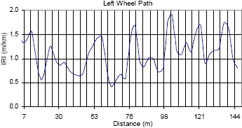
1 m = 3.28 ft 1 m/km = 63.4 inches/mi

Figure 127. Roughness profiles for I-69, right wheel path.

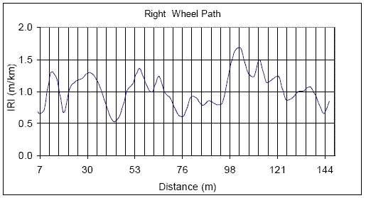
1 m = 3.28 ft 1 m/km = 63.4 inches/mi

Figure 128. Roughness profiles for I-69, left and right wheel path.

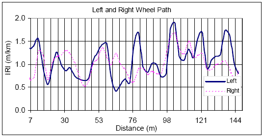
1 m = 3.28 ft 1 m/km = 63.4 inches/mi

Coefficient of Thermal Expansion and Microscopical Examination

A CTE test was conducted on a 150-by-300-mm (5.9-by-11.8-inch) core from the pavement. The CTE value for the specimen was 8.25 x 10^-6 per ^oC (4.58 x 10^-6 per ^oF). A microscopical examination of the core indicated that the coarse aggregate was dolomite/dolomitic limestone (carbonate) and the fine aggregate was silicious.

Summary

• Testing performed immediately after paving indicated that the left and right wheel path IRI were very close to each other; the values from day-1 testing were 1.15 and 1.17 m/km (73 and 74 inches/mi), respectively.
• When IRI obtained from the three repeat runs for the entire section were evaluated for all data sets collected by the lightweight profiler, the average of the difference between the maximum and minimum IRI was 0.04 m/km (2.5 inches/mi).
• An evaluation of short-interval IRI repeatability of the lightweight profiler using 15-m (49-ft) segment lengths indicated that the average difference between the maximum and minimum IRI obtained from the repeat runs was 0.11 m/km (7 inches/mi).
• The method used to form joints in this project was similar to that used at the test section on U.S. 23. The lightweight profiler used to collect profile data at this test section was the same device that collected data at the test section established on U.S. 23. The observations regarding the condition of the joint on profile data and roughness indices noted at this section were similar to those at the test section on U.S. 23.
• A reduction in IRI from that obtained at 1 day was seen for data collected on day-6 and day- 10 morning (joint reservoir was not sawed at this time). The reduction in IRI ranged from 4 to 11 percent for the different wheel paths and test dates. The joints in the pavement had been sawn just before profile data collection on the first day the pavement was profiled, and residue from the joint sawing operation was present adjacent to the joints at the time of profiling. Hence, the higher IRI obtained for day 1 may have been due to this residue.
• IRI obtained after the joint reservoirs were formed - but the joints not sealed - was much higher than that obtained from data collected when only the initial sawcut was present on the pavement. The IRI values obtained when the joint reservoir was sawed but joint not sealed were higher than the IRI obtained before forming the reservoir by 18 and 42 percent for the left and the right wheel paths, respectively. The joint reservoir was noted to have had a higher depth along the right wheel path than the left, which was the cause for the higher increase in IRI along the right wheel path. Profile data were not collected immediately after the joints were sealed; hence, a comparison of IRI values obtained after the joints were sealed could not be performed.
• IRI obtained 4.5 months after paving was higher than the 1-day IRI by 9 percent and 22 percent along the left and the right wheel paths, respectively. The 1-day profiling was performed with a lightweight profiler, whereas the 4.5-month profiling was performed with a high-speed profiler. It is unclear whether the difference in IRI was caused by a change in the pavement profile or whether it was related to differences between the two profilers' data collection capabilities. Also, a median barrier was present when the 4.5-month data were collected, and the path followed by the high-speed profiler during profiling may have been different from that followed by the lightweight profiler. This situation might also be a contributing factor to differences in IRI.
• Apart from the RN values obtained when the joints were in an unsealed condition with the joint reservoirs sawed, little change in RN occurred for the other profiling times that varied from 1 day after paving to 4.5 months after paving. When all profiling paths and test sequences were considered, the changes in RN that occurred compared to the 1-day RN ranged from -6 to 7 percent.
• There was negligible curvature in the PCC slabs. No noticeable changes in curvature were noted over the monitored period.