Volume 2, Chapter 4

Introduction

A second method used to demonstrate the Level 1 PRS prototype specification involved developing general pay factor charts for typical designs within a chosen SHA. As a follow-up to the original shadow field trial, the research team developed Level 1 pay factor charts representative of three typical pavement designs used in Iowa. The objectives of this exercise were twofold:

1. To demonstrate how the Level 1 prototype approach can be used by a SHA to develop pay factor charts for commonly used designs—each chart being specific to a particular road classification and climatic region.

2. To illustrate an example of the trends that may occur between different pay factor charts developed for different pavement classes.

This chapter explains the details of selecting the different pavement designs, the development of the respective pay factor charts, an analysis of the observed trends within and between the developed charts, and the conclusions and recommendations resulting from this exercise.

Defining Three Different Pavement Designs

The first step was the selection of three typical PCC pavement designs used in Iowa. Each pavement design was selected to be specific to an assumed traffic level representing medium, heavy, or very heavy traffic. All three pavement designs were assumed to have a 40-year design life. The chosen cumulative ESAL values (over the 40-year design lives) for each of the chosen traffic classifications consisted of the following:

• Medium Traffic: 2.5 million ESAL’s
• Heavy Traffic: 7.5 million ESAL’s
• Very Heavy Traffic: 30.0 million ESAL’s

Definition of Pavement Performance

For the development of these pay factor charts, pavement performance was defined in terms of all of the four available distress indicators (i.e., transverse slab cracking, transverse joint faulting, transverse joint spalling, and pavement smoothness over time).

Selection of Acceptance Quality Characteristics

For the three chosen typical designs, Level 1 pay factor charts were developed for each of the following four AQC’s:

• Concrete Strength.
• Slab Thickness.
• Entrained Air Content.
• Initial Smoothness.

Selection of Representative Constant Values

The representative constant values required to simulate the corresponding pay factor charts (for the three chosen designs) were determined based on information provided by Iowa SHA personnel. Values for the climatic-related variables and unit costs were assumed to be the same as those used at the original PRS field trial conducted in Wapello County, Iowa, in 1996 (see chapter 2 of this volume). More information on the selection of constant variables is presented in chapter 5 of volume I, in the section titled Identification of Constant Variable Values. The specific values chosen to represent each of the three typical designs are presented in table 71. (Note: The constant inputs presented in table 71 are those required by the old distress prediction models used in the prototype PaveSpec software.^(1-3) These variables differ slightly from those constant values required by the new distress indicator models included in the revised PaveSpec 2.0 software [as shown in figure 1 of volume I].)

Table 71. Chosen constant variable values for the required PRS inputs for three typical pavement designs in Iowa.

Variable		Design 1 (Medium Traffic)	Design 2 (Heavy Traffic)	Design 3 (Very Heavy Traffic)
Project Information
	Pavement Type	Doweled, JPCP
	Road Location	Rural Setting
	Highway Type	Undivided	Divided	Divided
	Design Life	40 years
	No. of Lanes in One Direction	1	2	2
	Lane Width	3.7 m
	Joint Spacing	6.1 m
Traffic Information
	Total Design Traffic	2.5 MESAL’s	7.5 MESAL’s	30.0 MESAL’s
	Initial Year Traffic	62,500 ESAL’s	187,500 ESAL’s	750,000 ESAL’s
	Traffic Growth Type	Simple Linear Trend
Materials and Climatic Information
	Annual Temperature Range	22 ºC
	Freezing Index	750 degree-days
	Average Annual Precipitation	81.3 cm
	Projected Annual Freeze-Thaw Cycles (at 7.6 cm below the pavement surface)	12
	Salt Present	Yes
	Joint Sealant Type	Liquid Asphalt
Slab Support Information
	Base Type	Granular
	Modulus of Subgrade Reaction	40.7 MPa/m
	Subgrade Soil Type	Fine-grained (AASHTO A4-A7)
	Presence of Longitudinal Subdrains	Yes
Load Transfer Information
	Dowel Bar Diameter	3.2 cm	3.8 cm	3.8 cm
	Presence of Tied PCC Shoulder	Yes
Cost Information
	Construction Bid, Traffic Lanes (based on $86.32/m3)	$17.89/m2	$20.08/m2	$23.32/m2
	Cost of Asphalt Overlay	$10.76/m2
	Cost of Patching a Joint	$95.68/m2
	Cost of Replacing a Slab	$83.72/m2
	Assumed Asphalt Overlay Life	20 years

Selection of AQC Target Values

Four different AQC’s were chosen to demonstrate the Level 1 PRS approach for each of the three typical designs. These included 28-day flexural strength (third-point loading), slab thickness, plastic entrained air content (using a pressure meter), and initial smoothness (measured using a 5.1-mm blanking band). The AQC target means and standard deviations for each of the three designs were estimated by interpreting the current Iowa construction specifications. These values were determined using the same procedures utilized in determining the target values at the original Iowa field trial in 1996 (see the section titled Definition of the Required As-Designed AQC Target Values in chapter 2 of this volume). The chosen AQC as-designed target means and standard deviations are presented in table 72 (the actual specification design thickness means are shown as a comparative reference).

Table 72. Chosen AQC as-designed target values for three typical pavement designs in Iowa.

Selection of Simulation Parameters

A number of simulation-related parameters are required to simulate LCC’s representing the as-designed and as-constructed pavement lots. The individual Level 1 AQC pay factor charts were simulated using the following simulation parameters:

• 80-year analysis life (twice the 40-year design life).
• 4 sublots per lot.
• 4 samples per sublot (for each AQC).
• 100 simulated lots for each simulated LCC.
• 5 percent of the computed user costs are included.

These simulation parameters are used in conjunction with the defined constant variable values and selected AQC target values to generate the preconstruction output.

Simulation of AQC Pay Factor Charts and Corresponding Pay Factor Equations

The final step in the specification development process involves the development of the preconstruction output. For the Level 1 specification, this involves constructing individual pay factor charts (and corresponding pay factor equations) for the four AQC’s. Individual AQC pay factors may be computed using these equations by knowing the as-constructed AQC lot means and standard deviations. (Note: Each pay factor chart is specific to the chosen constant values, target means, and standard deviations.)

Step-by-Step Procedure Used to Develop Individual Level 1 AQC Pay Factor Curves

The following step-by-step procedure was used to develop Level 1 pay factor charts and corresponding pay factor equations for the three typical Iowa designs. (Note: Each of these steps is accomplished using the PaveSpec PRS demonstration software.)

1. Define the number of sublots per lot. As mentioned previously, four sublots

2. Define the number of samples per sublot. A sampling frequency of four samples per sublot was used for each of the four AQC’s. In a Level 1 PRS, we assume that all of the material in a lot is represented by the same statistical population. Based on this assumption, the total sample size N may be represented by the number of sublots, n, times the number of samples per sublot. Therefore, the total sample size N was 16 for the case of 4 sublots.

3. Define the Level 1 AQC target means and standard deviations. The Level 1 target as-designed AQC means and standard deviations for the three typical designs were defined in table 72.

4. Choose a range of as-constructed means for each AQC. Reasonable ranges of AQC means are selected that will define the values used in the PaveSpec simulations. These chosen ranges of AQC simulation means (based on the chosen AQC target values for each of the three designs) are presented in table 73.

Table 73. As-constructed AQC simulation mean ranges for the three typical

AQC	Design 1 (Medium Traffic)	Design 2 (Heavy Traffic)	Design 3 (Very Heavy Traffic)
28-day Flexural Strength (third-point loading), MPa	3.78 – 5.18
Slab Thickness, mm	187 – 227	213 – 253	251 – 291
Entrained Air Content, %	0.0 – 7.0
Initial Smoothness (5.1-mm blanking band), mm/km	0 – 240

5. Choose specific as-constructed AQC standard deviation levels for the simulation of pay factor curves. The pay factor curves not only depend on the as-constructed AQC mean, but the as-constructed AQC standard deviation as well. Table 74 contains the three different standard deviation levels chosen (for each AQC) representing very good, good, and poor AQC quality control. These different levels of AQC standard deviation are used in the simulation of individual AQC pay

Table 74. As-constructed AQC standard deviation levels for simulation

AQC	Design 1 (Medium Traffic)	Design 2 (Heavy Traffic)	Design 3 (Very Heavy Traffic)
28-day flexural strength (third-point loading), MPa	0.00, 0.45, 0.90
Slab thickness, mm	0, 6, 13
Entrained air content, %	0.0, 0.5, 1.5
Initial smoothness (5.1-mm blanking band), mm/km	0, 16, 79

6. Simulate the target as-designed LCC’s. In order to calculate pay factors for different hypothetical levels of as-constructed AQC quality, the target as-designed LCC’s had to first be simulated. The PaveSpec specification simulation software was used to estimate target as-designed LCC means (for each of the 3 chosen designs) from 100 simulation lots, for the case of 4 sublots per lot and 4 AQC samples per sublot. Each individual lot was simulated by randomly selecting AQC samples from the target value distributions summarized in table 72. The simulations were conducted using an 80-year analysis life (twice the 40-year design life) and include 5 percent of the calculated user costs. The resulting simulated Level 1 mean as-designed LCC values (for the case of four sublots) for the three respective typical designs, were

• Design 1 (Medium Traffic): LCC_DES(1) = $668,709/km.
• Design 2 (Heavy Traffic): LCC_DES(2) = $706,135/km.
• Design 3 (Very Heavy Traffic): LCC_DES(3) = $722,795/km.

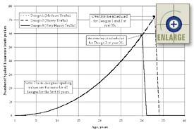
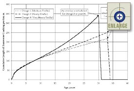
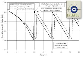
To better demonstrate the PRS method, the estimated typical distresses over time associated with each of the three Iowa designs (reflecting the chosen constant inputs and the AQC target means only) are presented in figure 14. These distresses reflect the predicted first overlay application at year 33 for Designs 1 and 2, and year 30 for design 3. The M & R plan defined for the original Iowa field trial was also used here.

Figure 14. Estimated typical as-designed distresses over time associated with each of the three typical designs (reflecting the chosen constant inputs and the AQC target means only).

7. Simulate as-constructed LCC’s and calculate an independent AQC pay factor for each hypothetical as-constructed mean/standard deviation pair. The hypothetical as-constructed mean/as-constructed standard deviation pair values (coming from combinations of means and standard deviations defined in steps 5 and 6, respectively) were used to define individual simulation sessions in the PaveSpec software. Each AQC was investigated independently for each session (for example, if strength was being investigated, all of the other AQC as-constructed means and standard deviations were set equal to the target values). Each pair was used in PaveSpec to simulate a corresponding LCC_CON. A pay factor was calculated for each pair using equation 5. The simulated pay factors (from PaveSpec) are summarized by AQC in tables 75 through 77.

Table 75. Design 1 (medium traffic)—simulated Level 1 pay factors for four sublots and four samples per sublot (lot sample size N=16).

Table 76. Design 2 (heavy traffic)—simulated Level 1 pay factors for four sublots and four samples per sublot (lot sample size N=16).

Table 77. Design 3 (Very Heavy Traffic)—simulated Level 1 pay factors for four sublots and four samples per sublot (lot sample size N=16).

8. Plot charts of pay factor vs. AQC mean. The simulated pay factors determined in step 7 can easily be graphed as a function of the AQC mean. Each AQC pay factor chart contains three different curves corresponding to the three different standard deviation levels chosen in step 5. Best-fit regression equations were fit through each individual pay factor curve representing one chosen as-constructed AQC standard deviation. Figures 15 through 17 contain AQC pay factor charts representing the three typical Iowa pavement designs. The best-fit pay factor regression equations (at different as-constructed AQC standard deviations) for the three chosen typical designs are summarized in tables 78 through 80. (Note: All of these charts and pay factor equations are specific to the assumed simulation parameters of four sublots per lot and four AQC samples per sublot.)

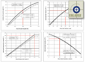Figure 15. Design 1 (medium traffic)—simulated Level 1 individual AQC pay factor charts for the case of four sublots per lot and four samples per sublot (lot sample size N=16).

Figure 16. Design 2 (heavy traffic)—simulated Level 1 individual AQC pay factor charts for the case of four sublots per lot and four samples per sublot (lot sample size N=16).

Figure 17. Design 3 (very heavy traffic)—simulated Level 1 individual AQC pay factor charts for the case of four sublots per lot and four samples per sublot (lot sample size N=16).

Table 78. Design 1 (medium traffic)—Level 1 AQC best-fit regression equations for the case of four sublots per lot and four samples per sublot (lot sample size N=16).

Table 79. Design 2 (heavy traffic)—Level 1 AQC best-fit regression equations for the case of four sublots per lot and four samples per sublot (lot sample size N=16).

Table 80. Design 3 (very heavy traffic)—Level 1 AQC best-fit regression equations for the case of four sublots per lot and four samples per sublot (lot sample size N=16).