Lab & Field Testing of AUT Systems for Steel Highway Bridges
6. RESULTS (cont'd)
The results from the second field test set at HSS are summarized in table 9. There were 14 field specimens in the second set. One specimen was designated as an FCM. RT and AUT inspections were performed on all specimens and an additional manual UT inspection was performed on the FCM specimen. RT and AUT inspection methods accepted the first 12 specimens in table 9. RT rejected field specimen G5G-TF1-TopF based on two slag inclusions found near the edge of the plate. The slag inclusions were 3.302 and 6.35 mm (0.13 and 0.25 inches) long and
23.876 and 487.426 mm (0.94 and 19.19 inches) from the datum, respectively. Figures 83
and 84 show photographs of field specimen G5G-TF1-TopF, with the datum assigned to the left edge of the plate. Figures 85 and 86 show the radiographic images of specimen G5G-TF1-TopF in two segments. The two slag inclusions in specimen G5G-TF1-TopF are not visible in figures 85 and 86 because of loss of resolution in the digitization process. Even though manual UT inspection was
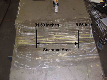
not required for specimen G5G-TF1-TopF, the fabricator conducted a manual UT inspection to determine the depth of the defects identified by RT. Again, this information allows for more efficient repairs. Note that the slag inclusions were found to be within code requirements according to the UT and AUT results. Figures 87 and 88 show the P-scan images of the weld in specimen G5G-TF1-TopF. The C-scan, B-scan, and end-view images show no rejectable indications. Therefore, the amplitude profile images in figures 87 and 88 show that the rejectable indications identified by RT are acceptable based on AUT. FCM field specimen G2G-CF1-BottF-FCM (figures 89 and 90) was required to be inspected using both RT and UT. RT accepted the specimen while UT and AUT rejected the specimen. Figures 91 through 94 show the radiographic images of specimen G2G-CF1-BottF-FCM in four segments. The P-scan images in figures 95 and 96 show a rejectable indication at approximately 635 mm (25 inches) from the datum. Manual UT inspection was conducted using 45-degree and 70-degree probes while the P-scan inspection was only performed with a 45-degree probe between Y = 224.8 mm and Y = 795 mm (Y = 8.85 inches and Y = 31.30 inches) due to time constraints.
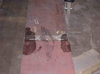
Figure 83. Field specimen G5G-TF1-TopF: Top view of joint. |
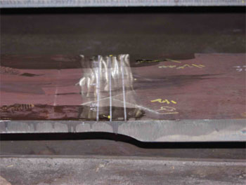
Figure 84. Field specimen G5G-TF1-TopF: Side view of joint. |
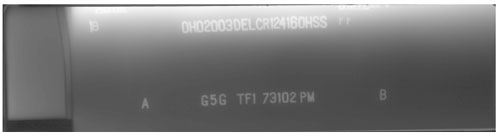
Figure 85. Radiographic image of field specimen G5G-TF1-TopF: Section A-B. |
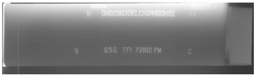
Figure 86. Radiographic image of field specimen G5G-TF1-TopF: Section B-C. |
Figure 87. P-scan images of field specimen G5G-TF1-TopF using 70-degree probe: From TSC side of centerline. |
 Figure 88. P-scan images of field specimen G5G-TF1-TopF using 70-degree probe: From BSC side of centerline. Figure 88. P-scan images of field specimen G5G-TF1-TopF using 70-degree probe: From BSC side of centerline. |
Figure
89. Field specimen
G2G-CF1-BottF-FCM: Top view of joint. |
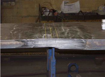
Figure 90. Field specimen G2G-CF1-BottF-FCM: Side view of joint. |
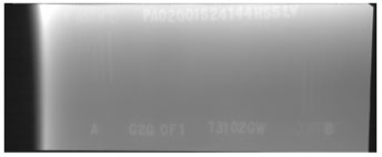
Figure 91. Radiographic image of field
specimen G2G-CF1-BottF-FCM: Section
A-B. |
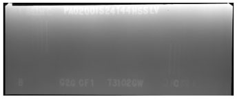
Figure 92. Radiographic image of field
specimen G2G-CF1-BottF-FCM: Section B-C. |
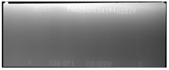
Figure 93. Radiographic image of field
specimen G2G-CF1-BottF-FCM: Section C-D. |
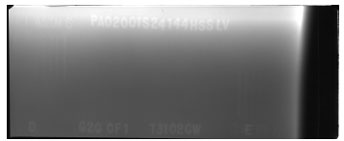
Figure 94. Radiographic image of field
specimen G2G-CF1-BottF-FCM: Section D-E. |
 Figure 95. P-scan images of field specimen
G2G-CF1-BottF-FCM using 45-degree probe: From TSC side of centerline.
Figure 95. P-scan images of field specimen
G2G-CF1-BottF-FCM using 45-degree probe: From TSC side of centerline. |
Figure 96. P-scan images of field specimen G2G-CF1-BottF-FCM using 45-degree probe: From BSC side of centerline. |
The results from the third set of field tests at HSS are summarized in table 10. The third test set consisted of 10 FCM field specimens and 2 HSS procedural test plates (TP2 and AWS-FCM-02-6A). Each HSS procedural test plate contains multiple realistic defects in the weld. The first six field specimens in table 10 were accepted by all three inspection methods. Specimens FG26G-TF2-BottF-FCM and FG16D-TF1-BottF-FCM were rejected by RT, but were accepted by manual UT and AUT. Photographs of specimen FG26G-TF2-BottF-FCM are shown in figures 97 and 98. Figure 99 shows the radiographic image of the weld with a rejectable 3.048-mm- (0.12-inch-) long slag inclusion at location Y = 286.77 mm (Y = 11.29 inches). The P-scan images in figures 100 and 101 indicate that the same rejectable slag inclusion identified by RT as rejectable is acceptable using AUT. Specimen FG16D-TF1-BottF-FCM (figures 102 and 103) was rejected by RT. The radiographic image in figure 104 shows that RT detected two slag inclusions. One slag inclusion was acceptable, while the other slag inclusion was rejectable. The P-scan images of specimen FG16D-TF1-BottF-FCM (figures 105 through 107) confirmed the presence of the two slag inclusions that were identified by RT. AUT identified these indications as being acceptable. Field specimen FG36K-TF2-TopF-FCM (figures 108 and 109) was rejected by all three inspection methods. RT detected a rejectable slag inclusion at Y = 857.25 mm (Y = 33.75 inches). However, the radiographic image of specimen FG36K-TF2-TopF-FCM (Figure 110) shows no visible defects because of loss of resolution during the digitization process. Note that the quality and the contrast of the radiographic image decreases for plates greater than 50.8 mm (2 inches) thick. Manual UT results (table 10) and P-scan images (figures 111 and 112) confirmed the presence of a rejectable slag inclusion. In addition, AUT also found multiple rejectable subsurface indications. Field specimen FG37K-TF3-BottF-FCM (figures 113 and 114) was accepted by RT, but was rejected by manual UT and AUT. Figure 115 is the radiographic image of weld section C-D, where a rejectable defect was found. The defect is not clearly visible in the radiograph because of loss of resolution during the digitization process. The P-scan image of weld segment C-D (Figure 116) shows a rejectable indication 10.414 mm (0.41 inch) long at Y = 677.418 mm (Y = 26.67 inches). The defect was 46.99 mm (1.85 inches) deep and was detected using a 45‑degree probe. Figure 117 shows that no rejectable indications were found in segment C-D using a 70‑degree probe. The first HSS procedural plate (TP2) (figures 118 and 119) was fabricated with four realistic slag inclusions in the weld. RT, manual UT, and AUT confirmed the presence of these rejectable slag inclusions. Unfortunately, a radiographic image was not available for TP2. The P-scan images of TP2 (Figure 119) indicate four rejectable indications. The second HSS procedural plate (AWS-FCM-02-6A) was rejected by all three inspection methods. Unfortunately, a radiographic image was not available for this specimen.
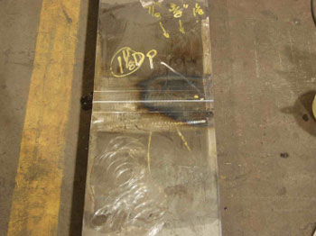
Figure 97. Field specimen FG26G-TF2-BottF-FCM: Top view of joint. |
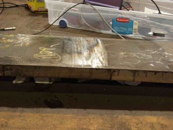
Figure 98. Field specimen FG26G-TF2-BottF-FCM: Side view of joint. |
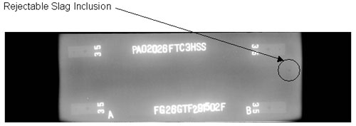
Figure 99. Radiographic image of field specimen FG26G-TF2-BottF-FCM. |
Figure 100. P-scan images of field specimen FG26G-TF2-BottF-FCM using 70-degree probe: From TSC side of centerline. |
Figure 101. P-scan images of field specimen FG26G-TF2-BottF-FCM using 70-degree probe: From BSC side of centerline. |
|


