Lab & Field Testing of AUT Systems for Steel Highway Bridges
6. RESULTS (cont'd)
The results of
the fourth set of field tests at HSS are summarized in table 11. There were
10 field specimens inspected; 5 of the 10 specimens were designated as
FCMs. Table 11 indicates that three FCM and three non-FCM specimens were
accepted with no rejectable defects by all of the inspection methods. The
76.2-mm- (3-inch-) thick field specimen FG40M-TF1-Curved-FCM (figures 120
and 121) is a plate specially fabricated for a railroad bridge. Unlike
conventional plates that are generally fabricated flat, specimen
FG40M-TF1-Curved-FCM was fabricated at a right angle. RT accepted the weld with
no rejectable defects. Since specimen FG40M-TF1-Curved-FCM is an FCM, it is
required to be inspected by UT. Two rejectable indications were detected by
manual UT and one rejectable indication was detected by AUT. Figure 122 shows a
radiographic image of the weld section where UT detected rejectable
indications. Figures 123 through 130 show the P-scan images created by
scanning the weld with a 45-degree probe. The rejectable indication is located
between Y = 228.6 mm and Y = 457.2 mm (Y = 9 inches and
Y = 18 inches) (figures 125 and 126). According to table 6.2 in the
AASHTO/AWS D1.5M/D1.5: 2002 Bridge Welding Code,(1) a 76.2-mm- (3-inch-)
thick plate is required to be scanned by 45-degree and 70-degree probes.
However, a P-scan inspection of the weld with a 70-degree probe was not
performed because of scheduling constraints. The 50.8-mm- (2-inch-) thick field
specimen FG1A-TF2-BottF-FCM (figures 131 and 132) was rejected by all three
inspection methods. RT rejected the specimen based on a rejectable slag
inclusion in section A‑B. According to table 6.2 in the AASHTO/AWS
D1.5M/D1.5: 2002 Bridge Welding Code,(1) a 50.8-mm- (2-inch-) thick
plate must be scanned by 60-degree and 70-degree probes. Manual UT and AUT
rejected the specimen based on an indication detected with the 60-degree and 70-degree
probes. The P-scan images of specimen FG1A-TF2-BottF-FCM, scanned with 60‑degree
and 70-degree probes, are shown in figures 133 through 135. Specimen
G3VHW-CF1-BottF (Figure 136) was rejected by RT based on a slag inclusion found
at location Y = 250.952 mm (Y = 9.88 inches). The
radiographic image of this weld section is shown in figure 137, but the
defect is not clearly visible. Manual UT and AUT inspection with a 70-degree
probe found an acceptable indication at Y = 250.952 mm (Y = 9.88
inches). Figure 138 shows the P-scan images from Y = 0 mm to
Y = 304.8 mm (Y = 0 inches to Y = 12 inches) for
specimen G3VHW-CF1-BottF. Field specimen G5VHW-CF1-BottF (figures 139 and 140)
was rejected by RT, but was accepted by manual UT and AUT. RT found a 6.35-mm-
(0.25-inch-) long slag inclusion at Y = 639.83 mm
(Y = 25.29 inches) (Figure 141). The defect is not clearly visible in
the radiographic image because of the poor quality of the radiographic film.
Specimen G5VHW-CF1-BottF was not required to be tested by manual UT; however,
the fabricator used UT to determine the depth of the defect for repair
purposes. Manual UT and AUT identified the defect found by RT and this
indication was found to be acceptable. The P-scan images from segment 4 in
specimen G5VHW-CF1-BottF were produced using 45-degree and 70-degree probes (figures
142 through 144). Figure 142 illustrates that the indication detected by AUT
was within code requirements.
The results of
the field tests at Stupp are summarized in table 12. There were four field
specimens tested, with all three inspection methods accepting all four
specimens.
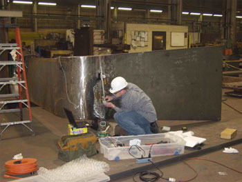
Figure 120. Field specimen FG40M-TF1-Curved-FCM: Top view of joint. |
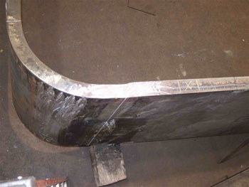
Figure 121. Field specimen
FG40M-TF1-Curved-FCM: Side view
of joint. |
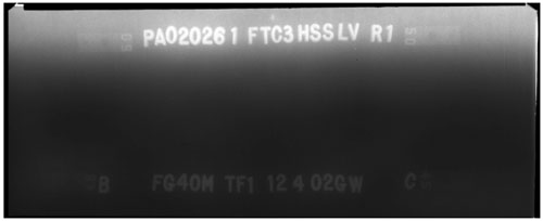
Figure 122. Radiographic image of field
specimen FG40M-TF1-Curved-FCM: Section B-C. |
Figure 123. P-scan images of field
specimen FG40M-TF1-Curved-FCM: From TSC side of centerline between 0 and
228.6 mm (0 and 9 inches). |
Figure 124. P-scan images of field
specimen FG40M-TF1-Curved-FCM: From BSC side of centerline between 0 and
228.6 mm (0 and 9 inches). |
Figure 125. P-scan images of field
specimen FG40M-TF1-Curved-FCM: From TSC side of centerline between 228.6
and 457.2 mm (9 and 18 inches). |
 Figure 126. P-scan images of field
specimen FG40M-TF1-Curved-FCM: From BSC side of centerline between 228.6
and 457.2 mm (9 and 18 inches). Figure 126. P-scan images of field
specimen FG40M-TF1-Curved-FCM: From BSC side of centerline between 228.6
and 457.2 mm (9 and 18 inches).
|
Figure 127. P-scan images of field
specimen FG40M-TF1-Curved-FCM: From TSC side of centerline between 457.2
and 685.8 mm (18 and 27 inches). |
 Figure 128. P-scan images of field specimen FG40M-TF1-Curved-FCM: From BSC side of centerline between 457.2 and 685.8 mm (18 and 27 inches). Figure 128. P-scan images of field specimen FG40M-TF1-Curved-FCM: From BSC side of centerline between 457.2 and 685.8 mm (18 and 27 inches). |
Figure 129. P-scan images of field
specimen FG40M-TF1-Curved-FCM: From TSC side of centerline between 685.8
and 993.8 mm (27 and 39.125 inches). |
Figure 130. P-scan images of field
specimen FG40M-TF1-Curved-FCM: From BSC side of centerline between 685.8
and 993.8 mm (27 and 39.125 inches).
|
Figure 131. Field specimen
FG1A-TF2-BottF-FCM: Top view of joint. |
Figure 132. Field specimen FG1A-TF2-BottF-FCM: Side view of joint. |
Figure 133. P-scan images of field specimen FG1A-TF2-BottF-FCM: From TSC side of centerline using 60-degree probe. |
Figure 134. P-scan images of field specimen FG1A-TF2-BottF-FCM: From TSC side of centerline using 70-degree probe. |
Figure 135. P-scan images of field specimen FG1A-TF2-BottF-FCM: From BSC side of centerline using 70-degree probe. |
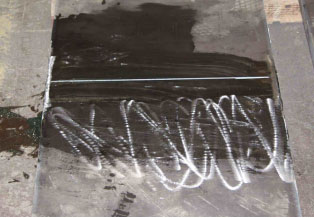
Figure 136. Field specimen
G3VHW-CF1-BottF: Top view of
joint. |
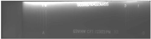
Figure 137. Field specimen G3VHW-CF1-BottF: Radiographic image of section A-B. |
Figure 138. Field specimen
G3VHW-CF1-BottF: P-scan
images from TSC side of centerline using 70-degree probe. |
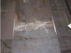
Figure 139. Field specimen G5VHW-CF1-BottF: Top view of joint. |
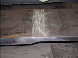
Figure 140. Field specimen G5VHW-CF1-BottF: Side view of joint. |
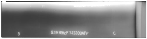
Figure 141. Field specimen G5VHW-CF1-BottF: Radiographic image of section B-C. |
Figure 142. P-scan images of field specimen G5VHW-CF1-BottF: From TSC side of centerline using 45-degree probe. |
Figure 143. P-scan images of field specimen G5VHW-CF1-BottF: From BSC side of centerline using 45-degree probe.
|
Figure 144. P-scan images of field specimen G5VHW-CF1-BottF: From BSC side of centerline using 70-degree
probe. |
For comparison,
the laboratory and field specimens with rejectable defects were grouped
according to plate thickness in 25.4-mm (1-inch) increments (tables 13 and 14).
These groupings summarized the results and helped determine the relationship
between the effectiveness of each inspection method with respect to the plate
thickness. The first column of each table shows the thickness range of the grouped
plates. The second column shows the total number of specimens inspected. The
third column indicates the number of specimens accepted with no rejectable
defects by all three inspection methods. The fourth column shows the number of
specimens rejected with rejectable defects by at least one inspection method.
The fifth column identifies the rejected specimen. The sixth column shows the
number of rejectable defects found. The seventh, eighth, and ninth columns
indicate the inspection methods that rejected the particular specimen. The
checkmark ( )
stands for "Rejected," indicating that the specimen was rejected by the
employed inspection method; X stands for "Accepted," indicating that the
specimen was accepted by the employed inspection method; and DWC stands for
"Detected/Within Code," indicating that the employed inspection method
identified an indication that was within code requirements. Table 13 shows that
the three inspection methods produced consistent results in the laboratory. In table
14, there are 8 field specimens with thicknesses ranging from 0 to 50.8 mm (0
to 2 inches) that contained 12 rejectable defects. RT rejected all eight
specimens, while UT rejected only three specimens. Note that UT identified
defects in the five remaining specimens, but found that the defects were acceptable.
In addition, 5 specimens with thicknesses ranging from greater than 50.8 to
101.6 mm (2 to 4 inches) containing 8 rejectable defects also were identified.
RT rejected only two specimens, while UT rejected all five specimens. Note that
FG36K-TF2-TopF-FCM was not rejected by AUT since the defect was located at the
curvature region of the width transition and the P-scan system was not configured
to inspect this type of region. )
stands for "Rejected," indicating that the specimen was rejected by the
employed inspection method; X stands for "Accepted," indicating that the
specimen was accepted by the employed inspection method; and DWC stands for
"Detected/Within Code," indicating that the employed inspection method
identified an indication that was within code requirements. Table 13 shows that
the three inspection methods produced consistent results in the laboratory. In table
14, there are 8 field specimens with thicknesses ranging from 0 to 50.8 mm (0
to 2 inches) that contained 12 rejectable defects. RT rejected all eight
specimens, while UT rejected only three specimens. Note that UT identified
defects in the five remaining specimens, but found that the defects were acceptable.
In addition, 5 specimens with thicknesses ranging from greater than 50.8 to
101.6 mm (2 to 4 inches) containing 8 rejectable defects also were identified.
RT rejected only two specimens, while UT rejected all five specimens. Note that
FG36K-TF2-TopF-FCM was not rejected by AUT since the defect was located at the
curvature region of the width transition and the P-scan system was not configured
to inspect this type of region.
Tables 15 and 16
compare the results of the RT and AUT inspections. The tables are arranged to
illustrate: (1) the total number of specimens inspected within each 25.4-mm (1-inch)
thickness increment, (2) the total number of specimens that were rejected by at
least one inspection technique, (3) the number of specimens rejected by each
inspection method, and (4) the number of specimens accepted with
identifiable indications.
Table 13. Consolidating the results of laboratory testing using laboratory
specimens with rejectable defects.
Thickness Range (inch) |
Total No. of Laboratory Specimens |
No. of Laboratory Specimens Accepted |
No. of Laboratory Specimens Rejected by at Least One Technique |
Rejected Laboratory Specimen |
Ind. No. |
Rejected by RT |
Rejected by UT |
Rejected by AUT |
0-1 |
6 |
0 |
6 |
S033 (0.5" thick) |
1 |
|
|
|
2 |
|
|
|
S034 (0.5" thick) |
1 |
|
|
|
2 |
|
|
X1 |
S125 (1" thick) |
1 |
|
|
|
2 |
|
|
|
3 |
|
|
|
S126 (1" thick) |
1 |
|
|
|
2 |
|
|
|
3 |
|
|
|
4 |
|
DWC |
|
S135 (1" thick) |
1 |
|
|
|
2 |
|
|
|
3 |
|
|
|
S136 (1" thick) |
1 |
|
|
|
2 |
|
|
|
>1-2 |
4 |
2 |
2 |
S132 (1.5" thick) |
1 |
|
|
|
S133 (1.5" thick) |
1 |
|
|
|
1AUT is not configured to detect transverse crack.
DWC: Detected/Within Code
1 inch = 25.4 mm
Table 14. Consolidating the results of field testing using field specimens with
rejectable defects.
Thickness Range (inch) |
Total No. of Field Specimens |
No. of Field Specimens Accepted |
No. of Field Specimens Rejected by at Least One Technique |
Rejected Field Specimen |
Ind. No. |
Rejected by RT |
Rejected by UT |
Rejected by AUT |
0-1 |
5 |
3 |
2 |
G5G-TF1-TopF (1" thick) |
1 |
|
DWC |
DWC |
2 |
|
DWC |
DWC |
TP2 (1" thick) |
1 |
|
|
|
2 |
|
|
|
3 |
|
|
|
4 |
|
|
|
| >1-2
|
23 |
17 |
6 |
FG26G-TF2-BottF-FCM (1.75" thick) |
1 |
|
DWC |
DWC |
FG16D-TF1-BottF-FCM (2" thick) |
1 |
|
DWC |
DWC |
AWS-FCM-02-6A (1.5" thick) |
1 |
|
|
|
FG1A-TF2-BottF-FCM (2" thick) |
1 |
|
|
|
G3VHW-CF1-BottF (1.75" thick) |
1 |
|
DWC |
DWC |
G5VHW-CF1-BottF (1.75" thick) |
1 |
|
DWC |
DWC |
| >2-3 |
13 |
9 |
4 |
FG36K-TF2-TopF-FCM (3" thick) |
1 |
|
|
X* |
2 |
X |
|
|
FG37K-TF3-BottF-FCM (3" thick) |
1 |
X |
|
|
FG38K-TF2-TopF-FCM (3" thick) |
1 |
|
|
|
2 |
X |
|
|
FG40M-TF1-Curved-FCM (3" thick) |
1 |
X |
|
|
2 |
X |
|
|
3-4 |
3 |
2 |
1 |
G2G-CF1-BottF-FCM (3.15" thick) |
1 |
X |
|
|
*AUT is not configured to detect transverse defects or inspect width transition regions.
1 inch = 25.4 mm
Table 15. Assessing the detectability and rejectability of three inspection methods in the laboratory.
Thickness Range (inch) |
No. of Laboratory Specimens With Rejectable Defects |
No. of Specimens Rejected by AUT |
No. of Specimens Accepted by AUT Within Code |
0-1 |
6 |
6 (100%) |
0 |
1-2 |
2 |
2 (100%) |
0 |
Table 16. Assessing the detectability and
rejectability of three inspection methods in the field.
Thickness Range (inch) |
Total No. of Field Specimens |
No. of Field Specimens With Rejectable Defects |
No. of Specimens Rejected by RT |
No. of Specimens Rejected by AUT |
No. of Specimens Accepted by RT Within Code |
No. of Specimens Accepted by AUT Within Code |
0-1 |
5 |
2 |
2
(100%) |
1 (50%) |
0 |
1 |
>1-2 |
23 |
6 |
6 (100%) |
2 (33%) |
0 |
4 |
2-3 |
13 |
4 |
2 (50%) |
4 (100%) |
0 |
0 |
3-4 |
3 |
1 |
0 (0%) |
1 (100%) |
0 |
0 |
ARTICULATION ANGLES
To supplement
field testing and establish the importance of the code-prescribed transducer
articulation, specimen S033 was tested at a series of fixed angles (0 degrees,
2.5 degrees, 5 degrees, 7.5 degrees, and 10 degrees). The angles were
measured with respect to a line normal to the weld centerline. The main purpose
of articulating the transducer is to obtain the highest possible amplitude echo
from a given defect. To accomplish this, the transducer must be articulated so
that the direction of the shear wave propagating within the specimen is perpendicular
to a plane of the defect. As mentioned earlier, specimen S033 (shown in figures
7 through 10) contained manufactured crack-like defects oriented along the
centerline in the weld bevels.
The testing is
performed by the P-scan system using a test frame (Figure 145) and a series of
wedges designed to keep the transducer at a fixed angle during scanning (Figure 146). Figure 146 shows an angled wedge attached to a vertical sliding bar which
is oriented transverse to the weld axis. The transducer is placed against the angled
wedge, holding the articulation angle fixed relative to the weld axis. As the
sliding bar is advanced along the length of the weld, the transducer is held at
the fixed angle of interest.
The maximum echo
amplitudes from the defect were determined from the P-scan images and were
plotted against the transducer articulation angles (Figure 147). The abscissa
in Figure 147 represents the transducer articulation angles, and the ordinate
represents the indication rating (d). The indication rating of negative dB is
indicative of a high-amplitude echo and the indication rating of positive dB is
indicative of a low-amplitude echo. It is evident from Figure 147 that the
amplitude of the echo decreases from a high value of -4 dB to a low value of
+14 dB as the articulation angle increases from 0 to 10 degrees, respectively.
The 0-degree articulation angle, which produces the highest indication rating
of -4 dB, reveals that the direction of the incident traveling wave is aligned
normal to the plane of the crack thus reflecting the highest amount of
ultrasonic energy. For articulation angles other than 0 degrees, the incident
traveling wave is no longer perpendicular to the plane of the crack, leading to
less ultrasonic energy reflection. The difference in the echo amplitude between
the articulation angles of 0 degrees and 2.5 degrees, 2.5 degrees and
5 degrees, 5 degrees and 7.5 degrees, 7.5 degrees and 10 degrees are
5 dB, 6 dB, 5 dB, and 2 dB, respectively. The 2-dB to 6‑dB
difference in the echo amplitude is significant in rejecting or accepting a
weld based on the indication rating criteria set forth in the UT
acceptance-rejection criteria in tables 6.3 and 6.4 in the AASHTO/AWS
D1.5M/D1.5: 2002 Bridge Welding Code.(1) Therefore, a rejectable
defect may be misrepresented as an acceptable indication if articulation of the
transducer is eliminated.
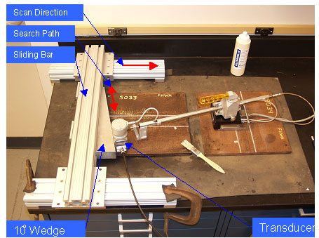 Figure 145. Transducer articulation testing: Test setup.
 |
Figure 146. Transducer articulation testing: Various articulation angle wedges. |
Figure 147. Influence of transducer articulation angle on the maximum amplitude of the reflected signal. |
|


