• Federal Highway Administration >
• Publications >
• Research Publications >
• 09020 >
• Chapt4.Cfm >
• Corrosion Resistant Alloys for Reinforced Concrete

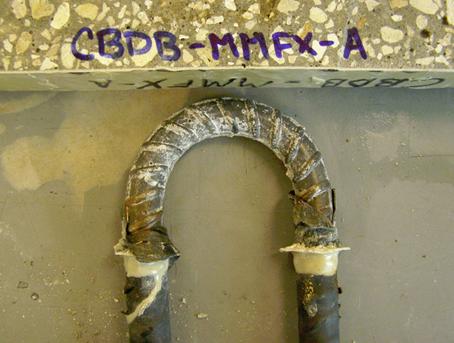
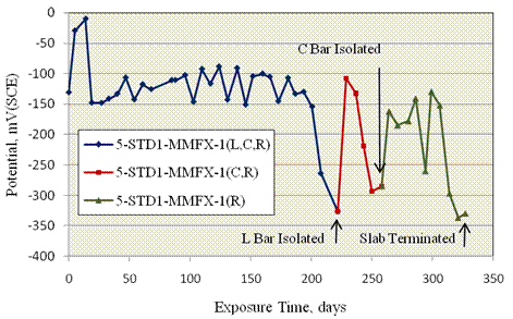
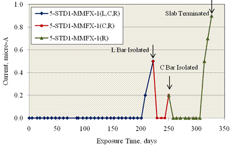
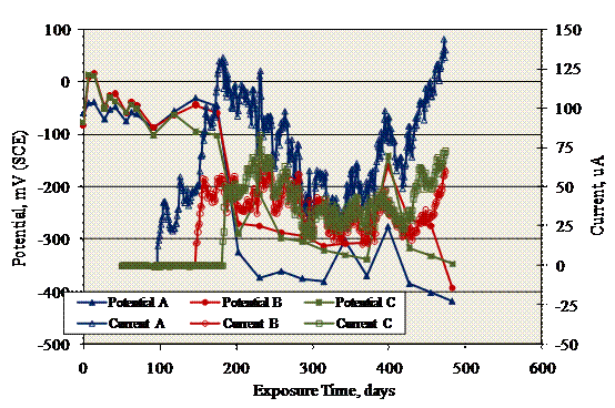
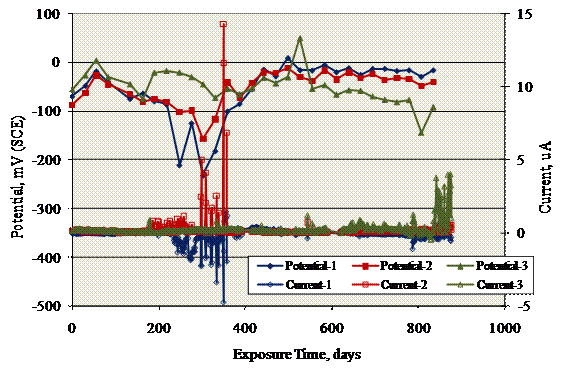
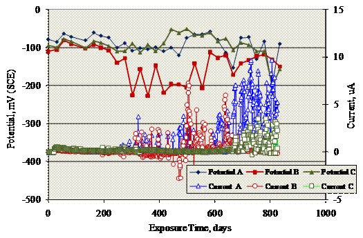
Corrosion Resistant Alloys for Reinforced Concrete

Previous | Table of Contents | Next

4.0 RESULTS AND DISCUSSION

4.1 Time-to-Corrosion

4.1.1 Results for Simulated Deck Slab Specimens

4.1.1.1 General Comments Regarding SDS Specimens

Results and discussion of the corrosion exposures are presented in two subdivisions. The first section, termed improved performance reinforcements, includes BB, 3Cr12, MMFX-2, and 2101. The second subdivision is termed high-performance reinforcements, which includes 316, 304, 2304, SMI, and STAX. This distinction between subdivisions was made because the former group of reinforcements initiated corrosion within the project timeframe, whereas most of the latter did not. Data for each of these are presented and discussed below.

4.1.1.2 Results for Improved Performance Reinforcements in SDS Specimens

Data for improved performance reinforced lot 5 specimens, which initiated corrosion, were employed for defining the respective T_i values. Figure 24 shows a typical plot of potential versus exposure time, while figure 25 plots macrocell current versus exposure time, in this case for MMFX-2 reinforced specimens. In general, the somewhat abrupt potential shift from relatively positive to more negative was accompanied by the occurrence of measureable macrocell current (figure 25). The latter serves as the criterion for defining T_i for the bar in question and for its isolation from other bars, as explained previously. In all cases, a positive current indicates that the top layer of bars was anodic to the bottom layer.

Figure 24. Graph. Potential versus time for specimens reinforced with MMFX-2 steel indicating times that individual bars became active and were isolated (L-left bar; C-center bar; R-right bar).

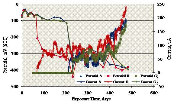
Figure 25. Graph. Macrocell current versus time for specimens reinforced with MMFX-2 steel indicating times that individual bars became active and were isolated (L-left bar; C-center bar; R-right bar).

Time-to-corrosion results for lot 5 specimens are listed in table 12. However, the procedure whereby individual bars were isolated was employed only after the 5-STD-BB slabs had become active and removed from testing. Upon dissection, all three bars in 5-STD-BB-1 and two in 5-STD-BB-2 and 5-STD-BB-3 were found to have locations of active corrosion. Bars without corrosion were treated as runouts. Also, if the extent of corrosion on a given bar was 25 mm or more wide, T_i was taken 8 days earlier than the time at termination. For example, specimen 5-STD-BB-1 was removed for exposure after 68 days. Upon dissection, the left (L) and center (C) bars where found to have corrosion products less broad than 25 mm, whereas for the right (R) bar, corrosion products were more extensive (width or length > 25 mm). While somewhat arbitrary, this data modification was thought to provide a more realistic representation of what occurred than if T_i for all bars had simply been taken as the slab termination time.

Table 12. T_i data for SDS/STD1 specimens with improved performance reinforcements (see table 4 for specimen designation nomenclature).

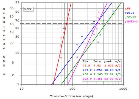
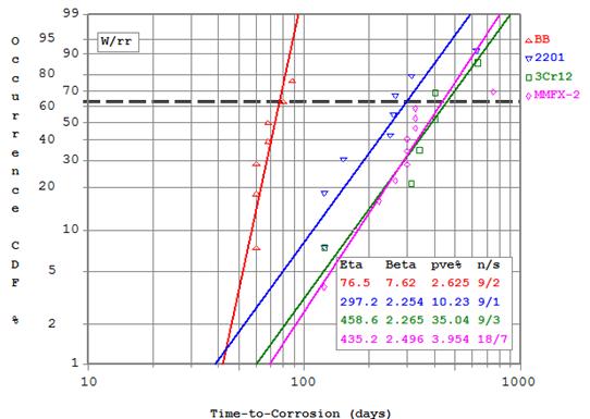
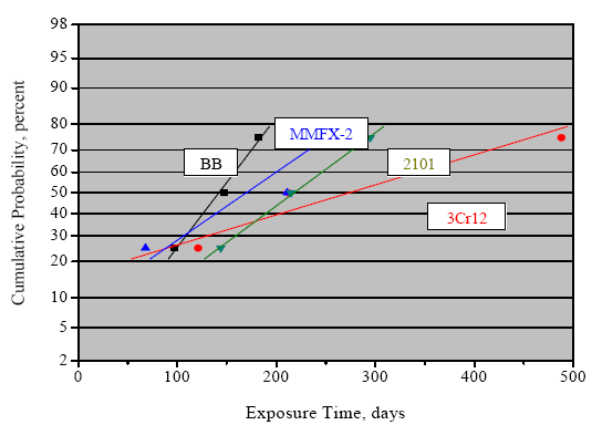
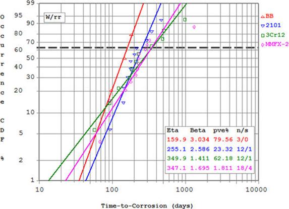
Figure 26 shows a cumulative distribution function (CDF) plot for the STD1 type specimen T_i data in table 12. Weibull statistics were employed because they take runouts into account in generating the best fit line, although the runout data per se are excluded from the plot. The mean T_i for these four reinforcements (the mean in Weibull statistics occurs at a CDF of 62.5 percent) is 76 days for BB, 459 days for 3Cr12, 306 days for MMFX-2, and 297 days for 2101.

Figure 26. Graph. Weibull cumulative distribution plot of T_i for the four indicated reinforcements.

In the figure, eta is the mean (dashed horizontal line), beta is a measure of data spread or slope of the best fit line, pve% is a measure of the line fit to data, n is the total number of specimens, and s is the number of runouts. Table 13 lists T_i and the ratio of T_i for individual improved performance bars to BB at 2 percent, 10 percent, and 20 percent active. These percentages were selected to cover a range of values from when damage first occurred to when intervention may be required.

Table 13 . Listing of T_i for improved performance reinforcements and T_i ratio to BB for SDS-STD 1 specimens at 2 percent, 10 percent, and 20 percent active.

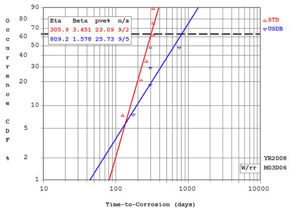
Figure 27 shows a CDF plot of T_i for the two types of specimens reinforced with MMFX-2, which includes STD and USDB (3-mm-diameter holes were drilled through the surface layer on the upper side of the top bars at 25 mm spacing). Here, the mean T_i for the STD specimens is 306 days and 809 days for the USDB specimens. It is unclear if this distinction is simply specimen-to-specimen scatter or if it reflects actual differences; however, no reason is apparent why surface damaged bars of this alloy should exhibit greater resistance to corrosion initiation than undamaged ones.

Figure 27. Graph. Weibull cumulative distribution plot of T_i for STD and USDB MMFX-2 reinforcements.

Figure 28 reproduces figure 26 but with both the STD and USDB MMFX-2 specimens included as a common data set. This transposes the MMFX-2 mean T_i from 306 days to 435 days, which is essentially the same as for 3Cr12 and at the upper bound for the alloys shown here.

Figure 28. Graph. Weibull cumulative distribution plot of T_i treating all STD and USDB-MMFX-2 reinforced specimens as a single population.

Referencing T_idata to the mean value has little practical significance because the mean value corresponds to widespread corrosion having occurred. For this reason, table 14 lists T_i values from figure 28 corresponding to 2 percent, 10 percent, and 20 percent probability of corrosion initiation, as well as the ratio of T_ifor each alloy to that for BB. Consistent with the large beta (less T_i scatter) in figure 28 for BB specimens compared to the three more CRR, the T_i ratio for each increased with increasing percent active. Thus, 3Cr12 and MMFX-2 were the better performers with T_i (alloy)/T_i (BB) near 2 at 2 percent active and 3.8 at 20 percent active.

Table 14. Listing of T_i for improved performance reinforcements and T_i ratio to BB for SDS-STD 1 specimens at 2 percent, 10 percent, and 20 percent active based on all MMFX-2 specimens.

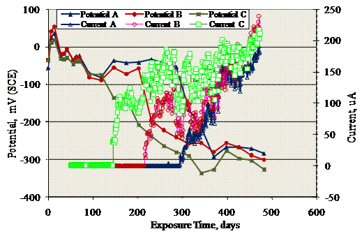
4.1.1.3 Results for High Performance Reinforcements in SDS Specimens

Table 15 lists exposure duration and macrocell current measurement results for the two types of 316SS (316.16.and 316.18, see table 1) reinforced SDS specimens that either did not initiate corrosion or that eventually did initiate corrosion on lower layer BB, as indicated by a negative macrocell current.

Table 15. Listing of exposure times and macrocell current data for Type 316SS SDS reinforced slabs.

-indicates that no specimen of the indicated type was fabricated.

Figure 29 shows a plot of macrocell current versus exposure time for specimens with a bottom BB mat.

Figure 29. Graph. Macrocell current history for 316 reinforced slabs with BB lower steel.

Table 16 lists data for Type 304SS reinforced slabs and indicates the same response as for the 316 (no macrocell current except for specimens fabricated with lower mat BB, which did eventually initiate corrosion).

Table 16. Listing of exposure times and macrocell current data for Type 304SS reinforced slabs.

- indicates that no specimen of the indicated type was fabricated.

Table 17 lists parameters and macrocell current measurement results for SDS slabs reinforced with STAX. The data indicate that isolated instances of measurable current occurred on occasion. However, for the most part, the macrocell current was 0 A. Specimen configurations for this reinforcement type were limited to those shown because of material stock limitations.

able 17. Corrosion activity for Stelax reinforced SDS specimens.

Results for SMI reinforced SDS slabs-other than those with a bar crevice, BB lower layer, concrete crack, or clad defects (or combinations of these)-are listed in table 18. In general, the macrocell current that occurred in some cases was small and infrequent.

Table 18. Listing of SMI reinforced SDS specimens and macrocell current results.

- indicates that no specimen of the indicated type was fabricated.

Table 19 lists the results for the other SMI specimens, which exhibited a distinct T_i. As indicated, T_i was 0 days for specimens of the CSDB condition (simulated concrete crack and 3-mm-diameter holes through the cladding spaced at 25-mm intervals on the top of upper bars), 20 days to 29 days for BCCD specimens (holes drilled through the cladding and BB bottom layer), and 139 days to 230 days for CVNC (top layer bars with a crevice and no caps on embedded bar ends).

Table 19. Results for SMI reinforced SDS specimens that exhibited a defined T_ifollowed by measureable macrocell corrosion.

Figure 30 provides a plot of macrocell current versus time for SDS-SMI specimen sets.

Figure 30. Graph. Current-time history for SDS-SMI specimens that initiated corrosion.

Three Type 2304SS reinforced STD1 specimens have been under test for 929 days with no macrocell current activity. Table 20 lists all high performance alloy reinforcement/specimen types that did not initiate corrosion within the exposure time and the corresponding ratio of T_i for each to the mean T_i for STD1 BB specimens (76 days, figure 24 and figure 26). Because exposure times were different for different specimen sets, the ratios vary from one alloy to the next but are as high as > 22.

Table 20. Ratio of T_i for CRR that did not initiate corrosion to the mean T_i for BB specimens.

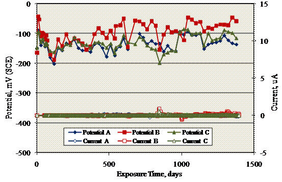
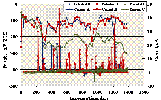
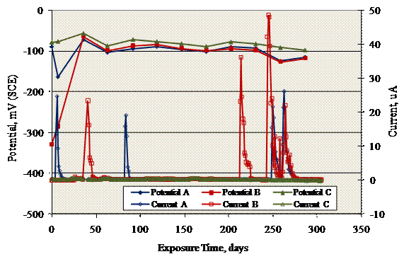
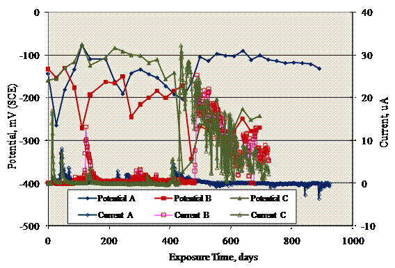
4.1.2 Results for Macrocell Slab (MS) Specimens

4.1.2.1 Results for Improved Performance Reinforcements in MS Specimens

Outdoor Exposures. The potential and macrocell current versus time trends for STD1-MS specimens with improved performance reinforcements were generally similar to those indicated previously for comparable SDS specimens (figure 24 and figure 25), as shown by figure 31 to figure 34. These plots show that macrocell current was nearly 0 mA initially but abruptly increased in most, but not all, cases; the potential correspondingly became more negative. Time-to-corrosion was defined for SDS specimens as initial occurrence of measureable, sustained macrocell current. Because there was only a single top bar (anode) for this specimen type, no bar isolation procedure was performed as was done for SDS specimens.

Figure 31. Graph. Potential and macrocell current results for MS-STD1-BB specimens.

Figure 32. Graph. Potential and macrocell current results for MS-STD1-3Cr12 specimens.

Figure 33. Graph. Potential and macrocell current results for MS-STD1-MMFX-2 specimens.

Figure 34. Graph. Potential and macrocell curent results for MS-STD-1-2101 specimens.

Table 21 lists the T_i values for MS-STD1 specimens reinforced with BB, 3Cr12, MMFX-2, and 2101.

Table 21. Listing of T_i values for MS-STD1 specimens with improved performance reinforcements.

Figure 35 shows a normal distribution CDF plot of T_i. In contrast to results for the SDS specimens (figure 26 and figure 28), the extent to which T_i was enhanced for the improved performance reinforcements in STD1 concrete is modest, particularly when corrosion initiation percentages were low, and the single 3Cr12 datum at 488 days was neglected.

Figure 35. Graph. Cumulative probability plot of T_i for STD1-MS specimens with improved performance reinforcements.

Table 22 shows T_i values for other STD1-MS specimen types reinforced with 3Cr12, MMFX-2, and 2101.

Table 22. Listing of T_i values (days) for MS specimens with improved performance reinforcements other than STD.

* Corrosion initiated at one or more lower black bars;
- indicates that no specimen of the indicated type was fabricated.

Table 22 shows T_i values for other STD1-MS specimen types reinforced with 3Cr12, MMFX-2, and 2201. Figure 34 shows a Weibull CDF plot of T_i that includes data for both the STD (table 21 and figure 36) and BENT, BNTB, BCAT, and USDB (table 22) specimen types based on the assumption that data for each alloy conform to a common population. The results show that T_i is approximately the same for all reinforcements at a relatively low activation percentage but with T_i for 3Cr12, MMFX-2, and 2101 diverging to slightly higher values as the active percentage increases. For specimens with a simulated crack (CBDB, CBNB, CBNT, and CCNB; table 22), corrosion initiated in less than 43 days for 3Cr12 and MMFX-2, but it was greater for 2101.

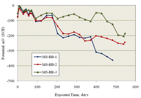
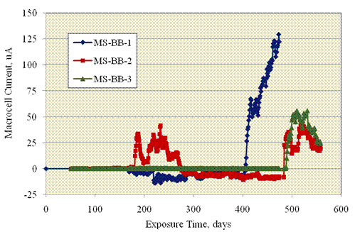
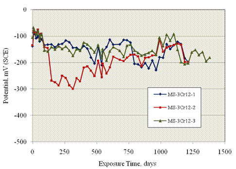
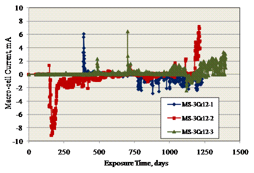
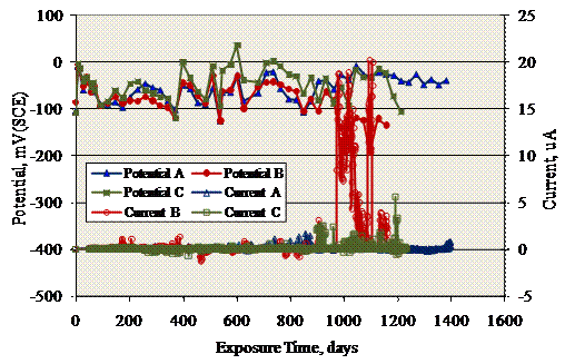
Figure 36. Graph. Weibull CDF plot of T_i for MS-STD1, -BCAT, -BENT, -BNTB, -UBDB, and -USDB specimens.

Data for STD2-MS specimens were not always conducive to definitively identifying T_i. Thus, figure 37 and figure 38 show potential and macrocell current data for the three BB MS specimens, and figure 39 and figure 40 show the data for the three 3Cr12 specimens. As for the SDS specimens, positive macrocell current corresponds to an anodic top bar. Corrosion was assumed to have initiated at the time at which this current increased to above the background level, which was near 0 mA. For MS-BB-1 in figure 38, a negative current occurred after 168 days, indicating that a lower bar (or bars) had initiated corrosion with the top bar serving as a cathode. This situation continued to 405 days, at which time the top bar activated and was anodic to the four lower bars. In the intermediate period, the top bar was cathodically polarized by one or more lower bars. This polarization is expected to have elevated the critical chloride concentration for corrosion initiation of the top bar. For MS-BB-2, corrosion initiated on the top bar after 180 days (positive macrocell current), but this polarity reversed at 275 days. These results indicate that a lower bar had activated, and its potential was more negative than that for the top bar. Corrosion of the top bar reinitiated after 483 days. Specimen MS-BB-3 behaved in a more conventional manner in that macrocell current was 0 mA until the top bar activated after 488 days.

In analysis of these data, a specimen was considered to have initiated corrosion upon initial occurrence of either a positive or negative current. For 3Cr12, current excursions were both positive and negative as for BB specimens, but they were smaller in magnitude and subsequently often reverted to near 0 mA, indicating repassivation. Specimen MS-3Cr12-1 was terminated after 1,233 days, and no corrosion was apparent upon dissection. Because of these complexities, data for 3Cr12 specimens was excluded in the T_i analysis. Specimens reinforced with MMFX-2 and 2101, on the other hand, exhibited better defined corrosion initiation for the top bar only. This is illustrated by figure 41 for STD2-MMFX-2 MS specimens, where specimen B initiated corrosion after 974 days, although the corresponding potential decrease was relatively modest (≤ 100 mV). Specimen C was removed after 1,221 days, and dissection revealed no corrosion. Specimen A remains under testing with no indication of corrosion initiation.

Figure 37. Graph. Potential versus time for STD2 black bar MS specimens.

Figure 38. Graph. Macrocell versus time for STD2 black bar MS specimens.

Figure 39. Graph. Potential versus time for STD2 3Cr12 MS specimens.

Figure 40. Graph. Macrocell current versus time for STD2 3Cr12 MS specimens.

Figure 41. Graph. Potential and macrocell current versus time for STD2 MMFX-2 MS specimens.

Based on the previously stated protocol, table 23 lists T_i values for the MS STD2 specimens. In the case of 3Cr12, one specimen was removed after 1,233 days and dissected; however, no corrosion was apparent. A second specimen apparently initiated corrosion after 1,181 days as an increase in macrocell current from near zero to a range of 4 A to 7 A occurred. The third specimen remains under test after 1,399 days with macrocell current in the range 0 A to 2 A. It is unclear if corrosion has initiated in this case.

Table 23. Listing of T_i values for MS-STD2 specimens with improved performance reinforcements.

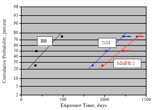
Figure 42 shows a CDF plot of T_iwhere data for 3Cr12 have been omitted because of the uncertainties mentioned previously. Corrosion initiation for BB specimens was considered to have occurred at the initial onset of macrocell current, either positive or negative. Runout data (indicated by arrows at data points in figure 40) were treated as if corrosion had initiated at the indicated time.

Figure 42. Graph. Normal CDF plot of T_ifor MS-STD2 specimens that exhibited a well-defined corrosion initiation.

Because of the limited data, it was necessary in generating this plot to treat runouts (two of the three MMFX-2 data and one of three for 2101) as having initiated corrosion at the time of termination, although either no corrosion was detected upon dissection of these specimens or the specimens remain under test. The data were insufficient for application of Weibull statistics. An attempt was made to project T_i (alloy)/T_i (BB), as was done above for SDS specimens; however, it was complicated by the fact that the best fit line through the three BB data points indicates negative T_iat small percentages active. For this reason, it was assumed that T_i at 2 percent, 10 percent, and 20 percent active was the value for the first BB specimen to become active (168 days). Doing this yields the T_i (alloy)/T_i (BB) results in table 24. However, if data for the lower percentages active were available, the ratios would be greater than indicated.

Table 24. Listing of T_i (alloy)/T_i (BB) for STD2-MS-MMFX-2 and -2101 reinforced specimens.

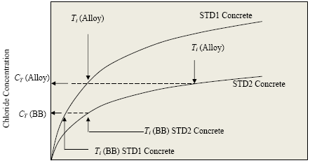
The higher values for these ratios compared to the STD1 results (table 21, figure 35, and figure 36) suggest that when comparing STD2 to STD1, better quality concrete (lower permeability) may be required to realize significantly greater T_ifor these improved performance reinforcements compared to BB. Figure 43 shows a schematic plot of [Cl^-] at a particular depth into concrete versus exposure time, assuming Fickian diffusional transport. The figure illustrates that T_i (alloy)/T_i (BB) for relatively low permeability concrete exceeds T_i (alloy)/T_i (BB) in high permeability concrete.

Figure 43. Chart. T_i for BB and an improved performance reinforcement in STD1 and STD2 concretes.

Controlled Temperature and Relative Humidity Exposures. Table 25 lists the T_i for individual specimens that underwent this exposure-all of which were of the STD1 mix design (designated STD1G in this case)-along with comparable STD1 data (table 21) and the average for each specimen type. This table shows that the average T_i for STD1G and STD1 was approximately the same for BB; however, for the three additional CRR, T_i for STD1G exceeded that for STD1. Variations in temperature and relative humidity, as occurred for the outdoor exposures, may have promoted sorptive transport of the ponding solution in the STD1 specimens, such that C_T was reached at the bar depth in a shorter time than for the STD1G specimens. It is possible that the relatively low C_T for BB specimens precluded this effect being apparent for this reinforcement.

Table 25. Listing of T_i for STD1G and STD1-MS specimens along with the three specimen average for each of the two exposures.

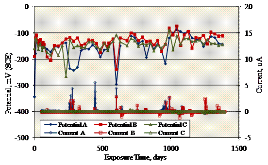
4.1.2.2 Results for High Performance Reinforcement in MS Specimens

Outdoor Exposures. Figure 44 to figure 48 show plots of potential and macrocell current versus time for 316.16SS, 316.18SS, 304SS, STAX, and SMI reinforced STD1-MS specimens. With the exception of the 316.16 data, for which macrocell current excursions were relatively small, the plots consist of occasional current "bursts" to as high as 38 A (figure 47) followed by repassivation. For STD2-MS-304, -316.16, and -316.18 specimens, macrocell current excursions were of lesser magnitude and more infrequent than for STD1. In the case of STD2-MS-SMI and -STAX, the excursions were about the same as for STD1.

Figure 44. Graph. Potential and macrocell current history for MS-STD1-316.16 specimens.

Figure 45. Graph. Potential and macrocell current history for MS-STD1-316.18 specimens.

Figure 46. Graph. Potential and macrocell current history for MS-STD1-304 specimens.

Figure 47. Graph. Potential and macrocell current history for MS-STD1-STAX specimens.

Table 26 lists the maximum and minimum currents that were recorded for the STD1 and STD2 specimens, where the positive current corresponds to the cathodic top bar to a lower bar (or bars) and negative to the anodic top bar.

Figure 48. Graph. Potential and macrocell current history for MS-STD1-SMI specimens.

Table 26. Listing of maximum and minimum macrocell currents for high alloy STD1-MS specimen.

Results for the other specimen types are presented according to type of reinforcement. Thus, table 27 lists the maximum and minimum macrocell currents for 316.16 reinforced specimens.

Table 27. Maximum and minimum macrocell currents for Type 316.16 specimens other than STD1 and STD2.

Figure 49 shows potential and macrocell current versus time for the CCNB specimens, which had the largest and most frequent current excursions. For 316.18, the only non-STD specimen type was CCON, for which the maximum and minimum macrocell currents were 7.0 A and -14.2 A, respectively.

Figure 49. Graph. Potential and macrocell current history for MS-CCNB-316.16 specimens.

Table 28 lists results for non-STD 304 reinforced specimens.

Table 28. Maximum and minimum macrocell currents for Type 304 specimens other than STD1 and STD2.

Figure 50 plots potential and macrocell current for the CCNB specimens with this reinforcement (same specimen type as for 316.16; see figure 49), which exhibited the largest current excursions.

Figure 50. Graph. Potential and macrocell current history for MS-CCNB-304 specimens.

Table 29 shows the maximum and minimum macrocell currents recorded for SMI reinforced specimens. For this alloy, the CSDB and USDB specimens exhibited relatively large current excursions.

Table 29. Maximum and minimum macrocell currents for SMI specimens other than STD1 and STD2.

Figure 51 and figure 52 show the time history for MS-CSDB-SMI speciments. For each reinforcement, the time of exposure is also shown because it varied for the different cases. Exposure time for 316.18 specimens was 1,387 days.

Figure 51. Graph. Potential and macrocell current history for MS-CSDB-SMI specimens.

Figure 52. Graph. Potential and macrocell current history for MS-USDB-SMI specimens.

Calculations were made to determine the corrosion rate associated with the current excursions. To do this, charge transfer was computed as the area under the current-time plots. The charge transfer served as input to Faraday's Law from which mass loss and wastage rate were determined.

Table 30 to table 40 show the results for specimens with relatively high charge transfer. In some cases, the calculations were made for both cathodic and anodic current excursions since these correspond to anodic activity on one or more of the lower bars. The columns labeled "Avg Corr Rate" list corrosion rates based upon the total exposure time, assuming wastage occurred uniformly over the entire exposed surface. For "Avg Corr Rate During Current Spike," the calculations were based on the time during which current excursions occurred. The column "Local Corr Rate," on the other hand, assumes that wastage during the macrocell current spikes occurred solely within a 1-mm² area such that the corrosion was localized, and all current activity occurred at the same location. While localization is likely, activation sites were probably random. Otherwise, successive activation and repassivation events would have occurred repeatedly at a single location. While this assumption is probably unrealistic, the calculation on which it is based does constitute a worst case situation. In most cases, this localized attack was at a rate of several mm/yr or less; however, for CSDB-MS-316.16-B, corrosion rate exceeded 22 mm/yr.

Table 30. Corrosion rate calculations for STD1-MS specimens with relatively high current excursions.

Table 31. Corrosion rate calculations for the STD2-MS specimens with relatively high current excursions.

Table 32. Corrosion rate calculations for CCON-MS specimens with relatively high current excursions.

Table 33. Corrosion rate calculations for BENT-MS specimens with relatively high current excursions.

Table 34. Corrosion rate calculations for the BCAT-MS specimen with relatively high current excursions.

Table 35. Corrosion rate calculations for CBNT-MS specimens with relatively high current excursions.

Table 36. Corrosion rate calculations for CBNB-MS specimens with relatively high current excursions.

Table 37. Corrosion rate calculations for CSDB-MS specimens with relatively high current excursions.

Table 38. Corrosion rate calculations for CCNB-MS specimens with relatively high current excursions.

Table 39. Corrosion rate calculations for CCNB-MS specimens with relatively high current excursions.

Table 40. Corrosion rate calculations for the BCAT-MS specimen with relatively high current excursions.

Controlled Temperature and Relative Humidity Exposures. Table 41 lists maximum and minimum macrocell currents for specimens in this category. Upon comparison to data in table 26, it is apparent that the magnitude of these was less than for specimens exposed outdoors. In most cases, only a single excursion was recorded. Apparently, variable temperature or humidity (or both) enhanced macrocell activity for the higher alloyed reinforcements to a greater extent than when temperature and relative humidity were controlled, although the magnitude of the effect was not of practical significance.

Table 41. Listing of maximum and minimum macrocell currents for MS-STD1G specimens.

Table 42 lists the high-performance reinforcement MS specimens that were tested. It also shows the T_i ratio for MS specimens to the average T_i for STD1-MS-BB specimens (142 days), assuming that the temporal current activity did not constitute corrosion initiation. Because exposure time varied depending on set number, the ratios also differed from one alloy to the next depending upon when testing commenced, with the largest ratio being >9.8.

Table 42. Listing of exposure times and T_i (alloy)/T_i (BB) for high performance reinforced MS specimens.

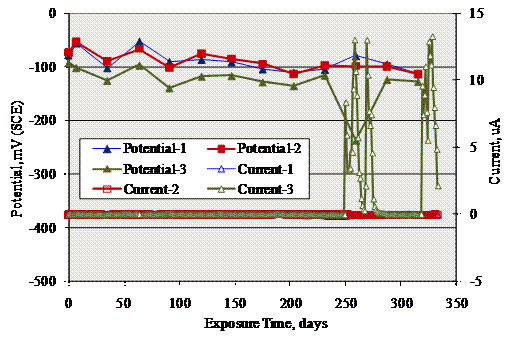
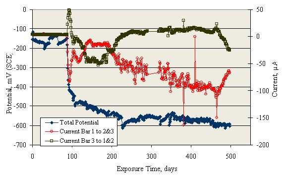
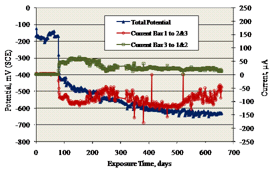
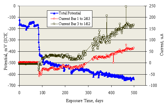
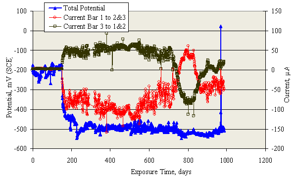
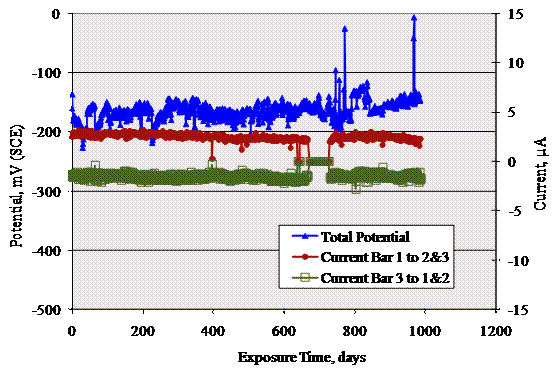
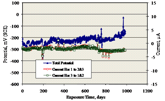
4.1.3 Results for 3-Bar Tombstone Column (3BTC) Specimens

4.1.3.1 Results for Improved Performance Reinforcements in 3BTC Specimens

As noted in section 3.3.4, either three or six standard 3BTC specimens of the STD2 and STD3 mix designs and selected reinforcement types were prepared. The potential of all of the bars that were connected as well as the voltage drop across the resistor between each long bar (designated as bar 1 and bar 2) and the other two bars (designation of the shorter bar was 3) were measured daily. Typical examples of the potential and macrocell current versus time behavior that were observed are illustrated by figure 53 to figure 56. In all cases, a relatively abrupt potential transition to more negative values occurred at a specific time, and this was considered as indicating corrosion initiation. Concurrently, a positive macrocell current excursion for one of the two measurement pairs and a negative excursion for the other were noted; however, the relative polarity of individual bars sometimes changed subsequently such that the macrocell current versus time trends conformed to one of several types of behavior. Thus, in figure 53 (3BCT-BB specimen A), the potential shift and corrosion current (bar 3) occurred at 89 days. However, after 102 days, current from bar 3 was cathodic and remained so until 224 days after which it was anodic until until 476 days. Current from bar 1, on the other hand, was cathodic subsequent to bar 3 activating.

The second example is provided by figure 54 (3BCT-BB specimen B), where corrosion initiated on bar 3 at 80 days with bar 1 serving as the cathode. The fact that the current for the former was less than for the latter indicates that bar 2 must also have been an anode. These relative polarities remained throughout the test. In figure 55 (3BTC-BB specimen D), corrosion initiated after 84 days with the current from both bars 1 and 3 initially being cathodic, indicating that bar 2 was the anode. However, the current from bar 3 to bar 1 and bar 2 reversed after 99 days such that it was now an anode as well and remained so thereafter. However, the current from bar 1 to bar 2 and bar 3 became anodic at 290 days. Lastly, in figure 56 (3BTC-BENT-3Cr12 specimen C), corrosion initiated after 152 days with positive current from bar 3 to bar 1 and bar 2. This demonstrated that bar 3 was an anode with a negative current from bar 1 to bar 2 and bar 3, indicating that bar 1 was a cathode. The current remained positive for bar 3 to 742 days, at which time it became an anode (positive current). Current from bar 1 to bar 2 and bar 3 was anodic for a period after 757 days. These polarities remained until day 838 for bar 1 and day 893 for bar 3, at which times, both currents reversed.

Figure 53. Graph. Potential and macrocell current between indicated bars for 3BCT-BB specimen A.

Figure 54. Graph. Potential and macrocell current between indicated bars for 3BCT-BB specimen B.

Figure 55. Graph. Potential and macrocell current between indicated bars for 3BCT-BB specimen D.

Figure 56. Graph. Potential and macrocell current between indicated bars for 3BCT-BENT-3Cr12-C.

Table 43 lists the improved performance 3BTC specimens, and it provides the T_i for each.

Table 43. Listing of 3BTC specimens with improved performance reinforcements and the T_i for each.

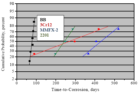
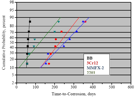
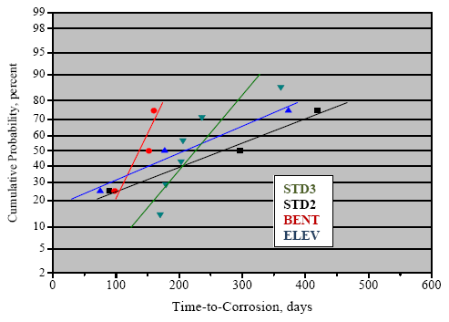
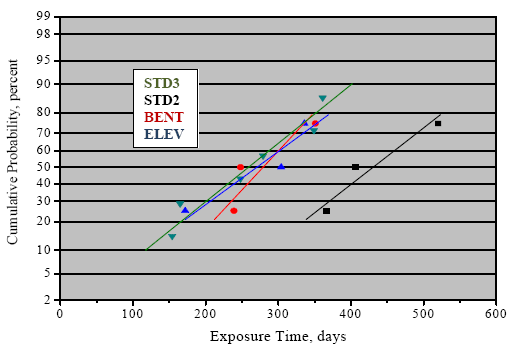
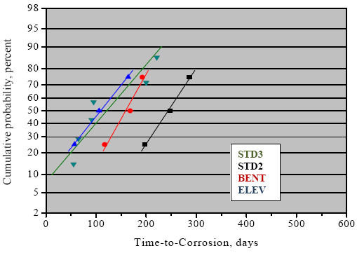
Normal cumulative distribution function plots of T_ifor 3BTC-BB, -3Cr12, -MMFX-2, and -2101 reinforcements in both concretes (STD2 and STD3) are presented in figure 57 to figure 61. The first of these (figure 57) illustrates T_i distribution for the reinforcements in STD2 concrete, and the next figure illustrates STD3.

Figure 57. Graph. Cumulative probability plot of T_i for 3BTC-STD2 specimens for each reinforcement.

Figure 58. Graph. Cumulative probability plot of T_i for 3BTC-STD3 specimens with each reinforcement.

Figure 59. Graph. Cumulative probability plot of T_ifor 3BTC-3Cr12 specimens.

Figure 60. Graph. Cumulative probability plot of T_i for 3BTC-MMFX-2 specimens.

Figure 61. Graph. Cumulative probability plot of T_i for 3BTC-2101 specimens.

Table 44 and table 45 list T_i and T_i (alloy)/T_i (BB) values at 2 percent, 10 percent, and 20 percent corrosion activity for the STD2 and STD3 3BTC specimens, as determined by extrapolating the best fit line for each specimen data set in figure 57 and figure 58. This determination was not made in cases where the extrapolation yielded an unrealistically low or negative T_i value. For all reinforcements, T_i is greater in STD2 than STD3 concrete, which is consistent with the former having lower w/c than the latter (0.41 compared to 0.50; see table 3). Also, the T_i ratio of each corrosion resistant reinforcement to BB at different percentages active was higher for the STD2 than STD3 concrete, which is consistent with results from the MS specimens. Thus, T_i (alloy)/T_i (BB) for MMFX-2 in STD3 concrete ranged from 0.9 to3.4. Whereas in STD2, it ranged from 3.7 to 5.2. The results indicate T_i ordering of these alloys relative to BB (highest to lowest) as MMFX-2 ≈ 3Cr12 > 2101 > BB.

Figure 59 to figure 61, on the other hand, plot normal CDF of T_i for the different bar configurations (straight, bent, and elevated) for 3Cr12, MMFX-2, and 2101 in STD3 concrete with the STD2 data included for comparison. In the latter two cases (MMFX-2 and 2101; figure 60 and figure 61), the difference in T_idistribution for the different bar configurations may be within the range of experimental scatter. The data are more distributed in the case of 3Cr12, however, with the ordering of T_i being (highest to lowest) STD2 > ELEV ≈ STD3 > BENT. Even here, it is unclear if the differences are real of if they simply reflect data scatter.

Table 44. T_idata and T_i (alloy)/T_i (BB) at 2 percent, 10 percent, and 20 percent cumulative active for improved performance 3BTC specimens in STD2 concrete.

- indicates that data for 2101 were not conducive for analysis.

Table 45. T_i data at 2 percent, 10 percent, and 20 percent cumulative active for 3BTC specimens with improved performance reinforcements in STD3 concrete.

- indicates that data for 2101 were not conducive for analysis.

Table 46 to table 48 list the T_i values at 2 percent, 10 percent, and 20 percent active according to the extrapolation of the best fit line in figure 59 to figure 61.

Table 46. T_idata at 2 percent, 10 percent, and 20 percent cumulative active for 3BTC specimens reinforced with 3Cr12.

- indicates that no STD2 or ELEV specimens were tested.

Table 47. T_i data at 2 percent, 10 percent, and 20 percent cumulative active for 3BTC specimens reinforced with MMFX-2.

Table 48. T_i data at 2 percent, 10 percent, and 20 percent cumulative active for 3BTC specimens reinforced with 2101.

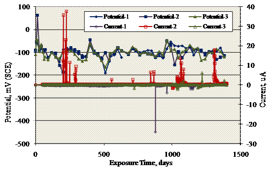
- indicates that no STD2 or ELEV specimens were tested.

4.1.3.2 Results for High Performance Reinforcements in 3BTC Specimens

For all high performance reinforcements that were included in 3BTC specimens (316.16, 304, and SMI), potential remained relatively positive for the duration of the exposures, and no sustained decreases occurred as was the case for specimens with improved performance bars. Figure 62 and figure 63 illustrate the two general types of macrocell current responses that were observed. In both cases, macrocell current, either from bar 1 to bar 2 and bar 3 or bar 3 to bar 1 and bar 2, was typically several microamperes starting from initial exposure. In the former case (figure 62), the two sets of current measurements are approximately the same magnitude but opposite sign, such that bar 3 was the anode, bar 1 was the cathode, and bar 2 provided little apparent contribution. For figure 63, however, both currents were negative, indicating that they served as cathodes to an anodic bar 2. Also, current spikes followed by repassivation are more apparent here than in figure 62. The latter behavior (figure 63) was more typical and reflects bar 2 having a more negative potential than bar 1 and bar 3, although all bars remained passive.

Figure 62. Graph. Potential and macrocell current versus time for 3BTC-SMI-specimen B in STD 3 concrete.

Figure 63. Graph. Potential and macrocell current versus time for 3BTC-316.16-ELEV specimen A.

Table 49 lists the maximum and minimum currents recorded during the exposure of each specimen. As for the higher alloyed MS specimens, corrosion rate associated with these current excursions was minimal.

Table 49. Maximum and minimum macrocell currents recorded for the high alloy reinforcement 3BTC specimens.

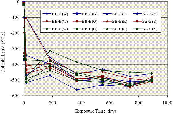
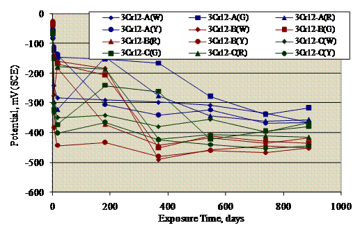
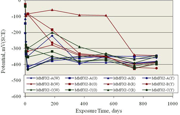
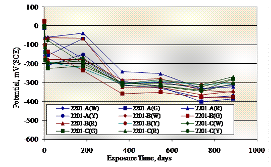
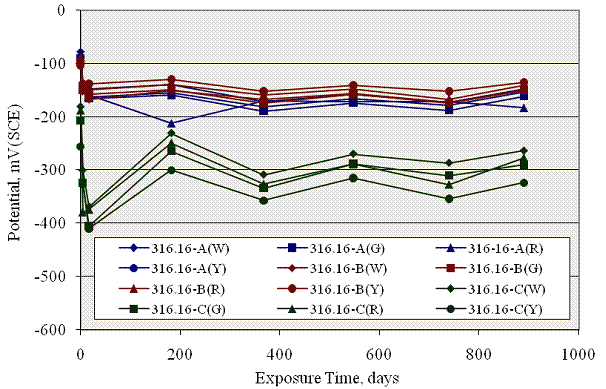
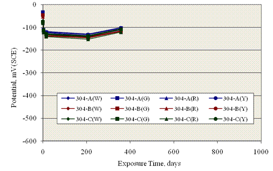
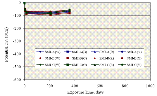
4.1.4 Results for Field Column Specimens

Figure 64 to figure 70 show potential versus exposure time plots for field column specimens with each type of reinforcement (BB, 3Cr12, MMFX-2, 2101, 316.16, 304, and SMI). The letters W, G, R, and Y in the specimen designation identify each of the four reinforcing bars in each column specimen. Data for the improved performance (3Cr12, MMFX-2, and 2101) and BB specimens (figure 64 to figure 67) exhibit a potential shift to relatively negative values. This often occurred within the first few days of exposure. The high permeability concrete (STD1 mix design) facilitated by rapid sorptive Cl^- transport and possible defects in the concrete or cracks caused the threshold concentration for this species to be achieved relatively early in the exposures. The potential time behavior for one of the three 316.16SS reinforced specimens (-C; see figure 64) was similar to that of the improved performance reinforced specimens. However, this particular specimen was damaged upon installation, and the negative potentials compared to the other two 316.16 reinforced specimens probably resulted from this.

Figure 64. Graph. Potential versus exposure time plot for field columns with BB reinforcement.

Figure 65. Graph. Potential versus exposure time plot for field columns with 3Cr12 reinforcement.

Figure 66. Graph. Potential versus exposure time plot for field columns with MMFX-2 reinforcement.

Figure 67. Graph. Potential versus exposure time plot for field column with 2101 reinforcement.

Figure 68. Graph. Potential versus exposure time plot for field columns with 316.16 reinforcement.

Figure 69. Graph. Potential versus exposure time plot for field columns with 304 reinforcement.

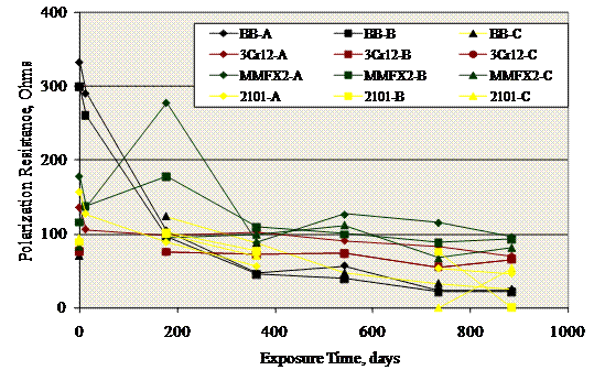
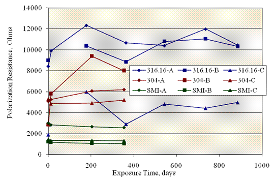
Figure 70. Graph. Potential versus exposure time plot for field columns with SMI reinforcement.

Results of the R_p determinations are presented in figure 71, which illustrates improved performance reinforcements, and in figure 72, which shows the high alloy results. For the former, R_p decreased with exposure time according to a generally common trend. Because corrosion rate is inversely proportional to R_p, the relatively low values are consistent with the corresponding potential data (figure 64 to figure 67) and support the likelihood that corrosion had initiated. Polarization resistances for the high performance bar specimens (figure 72) were generally more than an order of magnitude or more greater than for the improved performance bars. Also, these values remained relatively constant with time and ordered (high to low) as 316.16, 304, and SMI. Specimen 316.16-C, which was discussed previously, is an exception to this. Because surface area of the working electrode for the R_p measurements was unknown, the units are in ohms rather than the more conventional ohms per square centimeter.

Figure 71. Graph. Polarization resistance versus exposure time plot for field columns with improved performance reinforcements.

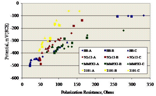
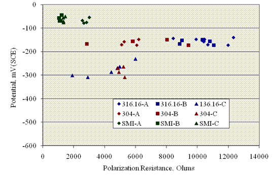
Figure 72. Graph. Polarization resistance versus exposure time plot for field columns with high alloy reinforcements.

Figure 73 and figure 74 show plots of R_p versus potential for the improved and high performance bar specimens. In the former plot, the data generally tracked from high R_p and relatively positive potential to low R_p and more negative potential, according to the decrease in both parameters as the exposures progressed. This trend is displaced somewhat to lower a R_p at a given potential for 2101 and to a higher R_p for MMFX-2. For the high performance specimens (figure 74), 316.16-C and 304-C exhibited potentials near -300 mV(SCE), whereas for other specimens, potentials were positive to -200 mV(SCE). The SMI bars have the most positive potentials compared to the other reinforcements in this category, despite R_p being relatively low. Because of the limited data, no attempt was made to estimate T_i for the different bar types.

Figure 73. Graph. Plot of polarization resistance versus potential for field columns with improved performance reinforcements.

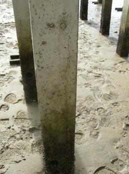
Figure 74. Graph. Plot of polarization resistance versus potential for field columns with high alloy reinforcements.

During each visit to the exposure site, researchers inspected the specimens for visible indications of corrosion damage and cracking. It was determined that each of the three BB field columns exhibited a crack in line with one of the four reinforcing bars after approximately 1 year of exposure. At the end of 2 years, each of the cracks had grown, and the three 2101 field columns also exhibited cracks. Table 50 summarizes observations at these two times, and figure 75 and figure 76 show photographs of cracking on a BB and 2101 reinforced field column specimen after 735 days of exposure.

Table 50. Summary of field observations for cracks that developed on field column specimens.

Figure 75. Photo. Cracking on a BB reinforced field column after 735 days of exposure.

Figure 76. Photo. Cracking on a 2101 reinforced field column after 735 days of exposure.

4.2 Critical Chloride Threshold Concentration for Corrosion Initiation, C_T

4.2.1 Chloride Analyses

Table 51 to table 57 list [Cl^-] analysis results for samples acquired both by coring and milling of SDS specimens. In all cases, [Cl^-] determined from milled samples was from locations along the bar trace where the reinforcement remained passive.

Table 51. Listing of [Cl^-] results for black bar reinforced specimens as acquired from coring.

Table 52. Listing of [Cl^-] results for 3Cr12 reinforced specimens as acquired from cores.

Table 53. Listing of [Cl^-] results for 3Cr12 reinforced specimens as acquired from millings.

Table 54. Listing of [Cl^-] results for MMFX-2 reinforced specimens as acquired from coring.

Table 55. Listing of [Cl-] results for MMFX-2 reinforced specimens as acquired from milling.

Table 56. Listing of [Cl^-] results for 2101 reinforced specimens as acquired from coring.

Table 57. Listing of [Cl^-] results for 2101 reinforced specimens as acquired from and milling.

Figure 77 plots [Cl^-] versus depth for all cores, and figure 78 to figure 80 show individual [Cl^-] versus depth data for both cores and millings for 3Cr12, MMFX-2, and 2101 specimens for which these determinations were made. The core data generally indicate decreasing [Cl^-] with depth into concrete as expected with differences in individual profiles, which were presumably a consequence of spatial concrete inhomogeneity. No trends are apparent from these data that suggest that differences in concrete age at the time of coring were a factor. Scatter of milling [Cl^-] data for individual specimens occured by a factor of 1.25 for 3Cr12 and 2101 specimens but 2.4 for MMFX-2; however, for individual MMFX-2 specimens, the range was 1.1 to 1.4. Differences in coarse aggregate volume percentage (CAVP) in the powder samples acquired by milling and the relatively small sample size (1.0-1.5 g) were probably responsible. Invariably, [Cl^-] for milled samples exceeded that for cores. This is attributed to a combination of the bar obstruction and CAVP effects.^(21,22,23)

Figure 77. Graph. Chloride concentrations as a function of depth into concrete as determined from cores taken from the indicated specimens.

Figure 78. Graph. Chloride concentrations determined from a core and millings for specimen 5-STD-1-3Cr12-2.

Figure 79. Graph. Chloride concentrations determined from a core and millings for MMFX-2 reinforced specimens.

Figure 80. Graph. Chloride concentrations determined from a core and millings for 2101 reinforced specimens.

4.2.2 Diffusion Coefficient and Chloride Threshold

Based upon the [Cl^-] data from individual cores (table 50 to table 55), values for the effective diffusion coefficient, D_e, were calculated using a least squares fit to the one-dimensional solution to Fick's second law (equation 3). They are listed in table 58 below.

Table 58. D_e values calculated from core [Cl^-] data.

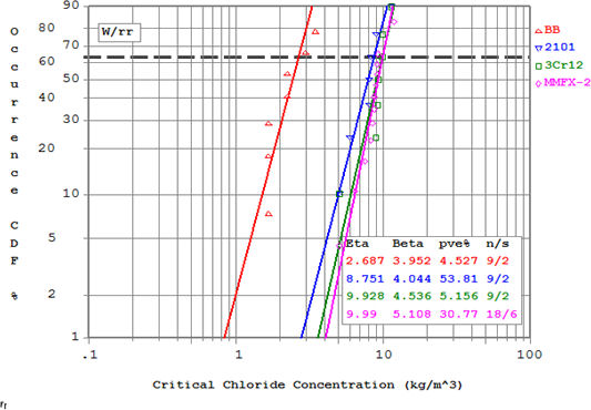
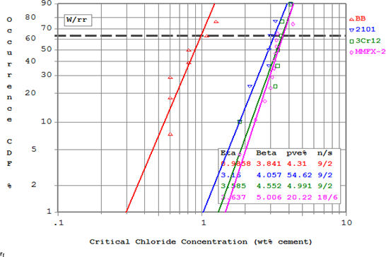
Using the average D_e ( 2.59∙10^-11 m²/s), C_T was calculated for each top bar of all of the improved performance specimens using equation 3, which is based upon T_i for each individual top bar and assuming C_s = 18 kg/m³ (7.22 cement wt percent basis). Figure 81 and figure 82 show Weibull CDF plots of C_T where for the former, C_T is in units of kg Cl^- per m³ of concrete, and in the latter, it is wt percent Cl^- referenced to cement.

Figure 81. Graph. Weibull cumulative distribution of C_T in units of kg Cl^- per m³ of concrete.

Figure 82. Graph. Weibull cumulative distribution of C_T in units of wt percent Cl^- referenced to cement.

Similar to what was done for the T_i data, table 59 lists C_T for each of the four steels at 2 percent, 10 percent, and 20 percent active. It also shows C_T (alloy)/C_T (BB) for 3Cr12, MMFX-2, and 2101. Values for the C_T ratio range from a low of 3.3 for 2101 at 20 percent active to a high of 4.8 for MMFX-2 at 2 percent active. These results are in general agreement with those of Clemeña and Virmani,⁽²⁴⁾ who reported values for C_T (alloy)/C_T (BB) as 4.7-6.0 for MMFX-2 and 2.6-3.4 for 2101 based upon slab experiments in 0.50 w/c concrete.

Table 59. Listing of C_T (kg/m³) for the improved performance reinforcements and black bar and C_T (alloy)/C_T (BB).

Minimal or no corrosion activity occurred for high alloy reinforcements except in conjunction with clad defects and perhaps crevices. Table 60 lists the five stainless steels in this category, the time each was exposed, and the corresponding [Cl^-] that is projected to be present at the bar depth based upon the diffusion analysis explained above (C_s = 18 kg/m³ and D_e = 2.59∙10^-11 m²/s). It is concluded that C_T for the individual bar types is greater than the indicated concentration.

Table 60. Projected [Cl^-] at the bar depth for the different reinforcement types after the indicated times.

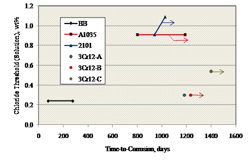
4.3 Comparison of C_T from Concrete Exposures and Accelerated Aqueous Solution Experiments

In the initial interim report for this project, an attempt was made to correlate C_T results from an accelerated aqueous solution test method with T_i data from lots 1-3 reinforced concrete exposures.⁽¹⁹⁾ The former method involved potentiostatic polarization at +100 mV (SCE) of 10 identical specimens of each reinforcement in synthetic pore solution (0.05N NaOH and 0.30N KOH of pH ≈ 13.2-13.25), to which Cl^- was incrementally added. The results indicated a general correlation in the two data sets but with large scatter, which may have resulted from the absence of heat shrink on the reinforcement ends. The possibility of such a correlation was revisited based upon results from set 5 SDS and MS specimen data. Figure 83 reproduces the aqueous solution accelerated C_T results reported previously, and table 61 lists the mean and standard deviation of these data for each alloy.

Figure 83. Graph. Previously reported chloride threshold concentrations as determined from aqueous solution potentiostatic tests.

Table 61. Listing of C_T data (wt percent) from accelerated aqueous solution testing.

Figure 84 plots these data versus those from the SDS-STD1 slabs for 10 percent and 20 percent active and the mean. The accelerated test data indicate that 2101 had the highest C_T of the four reinforcements. The SDS data, on the other hand, indicates that MMFX-2 and 3Cr12 had the highest C_T, although the difference between these and 2101 was small and may have been within experimental variability. However, the average accelerated test C_T data for 3Cr12 was about 60 percent below that for 2101 and MMFX-2. In the figure, the three successive data points with increasing threshold of each alloy correspond to 10 percent, 20 percent, and mean percent activation.

Figure 84. Graph. C_T determined from accelerated aqueous solution testing versus C_T from SDS concrete specimens.

Figure 85 provides a similar plot for STD-MS specimens where accelerated test C_T data at 20 percent and mean active are plotted versus T_i for the concrete specimens. The two successive data points with increasing T_ifor BB, MMFX-2, and 2101 correspond to 20 percent active and mean C_T, whereas the three 3Cr12 are the actual T_i values. Arrows on the MMFX-2 and 2101 data connecting lines indicate that one or both of the two respective points are runouts. These results are similar to those for the SDS-STD1 specimens in figure 84 where the accelerated aqueous solution results indicate C_T for 3Cr12 specimens were only slightly greater than the BB results and well below those for MMFX-2 and 2101. However, T_i for 3Cr12 concrete specimens was among the highest vales recorded. It is concluded that the accelerated test method did not adequately project performance of 3CR12 reinforcement in concrete.

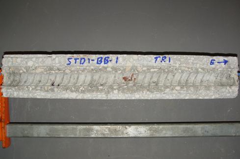
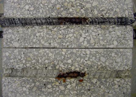
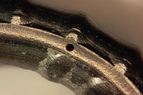
Figure 85. Graph. C_T determined from accelerated aqueous solution testing versus T_ifor STD2-MS concrete specimens.

4.4 Specimen Dissections

4.4.1 Dissection of SDS Specimens

Figure 86 is a photograph of a typical rebar trace upon the dissection of specimen 5-STD1-BB-1 2 weeks after detection of macrocell current. From the figure, a relatively small area of corrosion product is apparent. These observations are taken as confirmation of the experimental approach for defining T_i and C_T.

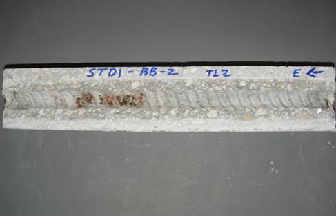
Figure 86. Photo. Upper R bar trace of dissected specimen 5-STD1-BB-1 showing localized corrosion products (circled).

Figure 87 shows an exceptional case where corrosion was more advanced prior to test termination.

Figure 87. Photo. Upper L bar trace of dissected specimen 5-STD1-BB-1 showing corrosion products.

In addition, dissections were performed on selected high performance reinforced specimens that either exhibited corrosion damage or were considered to potentially have corrosion. These specimens are listed in table 62 along with the exposure time at termination for each.

Table 62. Listing of high alloyed specimens that were autopsied.

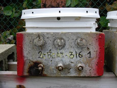
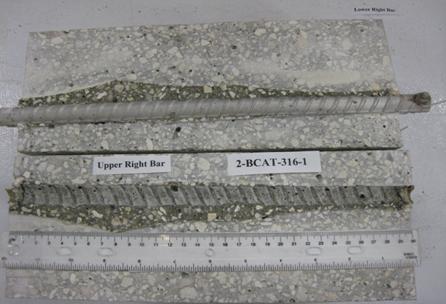
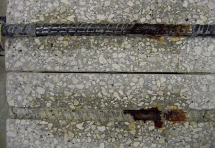
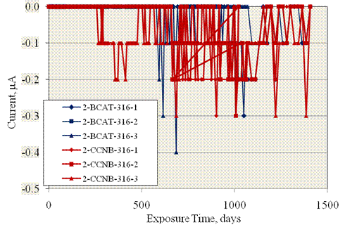
Figure 88 shows a side view photograph of specimen 2-BCAT-316-1 prior to dissection. Corrosion products are apparent extending from the BB on the lower left, and a thin concrete crack emanates from this and extends to the lower center bar.

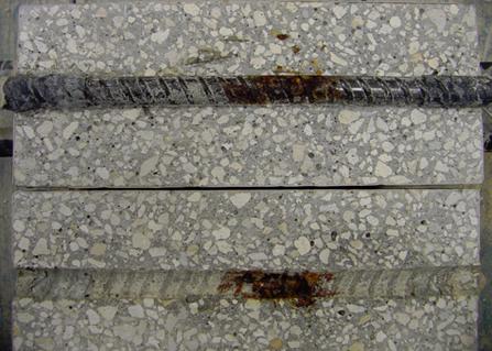
Figure 88. Photo. Specimen 2-BCAT-316-1 prior to dissection (red markings identify specimen for removal).

No corrosion was apparent upon dissection on any of the three top bars (figure 89); however, corrosion was extensive on the bottom BB (figure 90). The fact that corrosion appears most advanced at the bar ends indicates that absence of end sleeves was a contributing factor.

Figure 89. Photo. Top R bar and bar trace of specimen 2-BCAT-316-1 subsequent to dissection.

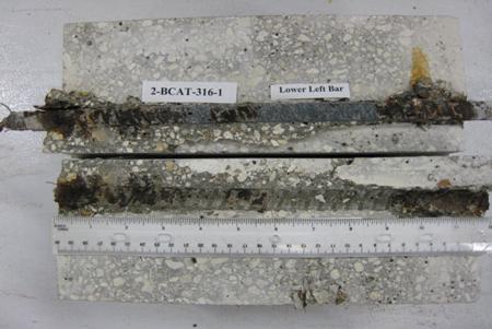
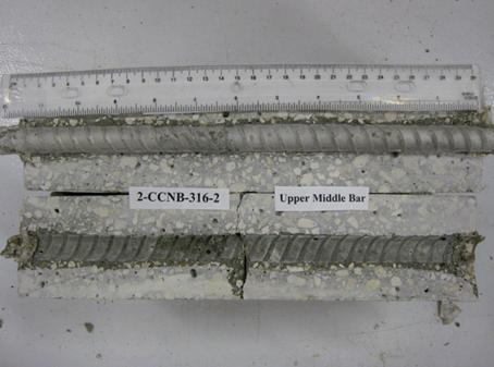
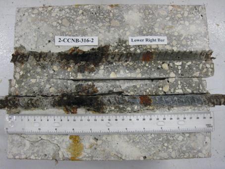
Figure 90. Photo. Lower L BB and bar trace of specimen 2-BCAT-316-1 subsequent to dissection.

Figure 91 shows a photograph of specimen 2-CCNB-316-2 prior to dissection. Although corrosion products are minimal, the concrete was delaminated along the plane of the bottom bars because of corrosion-induced cracking.

Figure 91. Photo. Specimen 2-CCNB-316-2 prior to dissection (red markings identify specimen for removal).

Minor staining was apparent on the top bars at locations beneath the simulated crack, as illustrated in figure 92. Concrete cracks that occurred during dissection are seen in the figure extending from the simulated crack.

Figure 92. Photo. Top C bar and bar trace of specimen 2-CCNB-316-2 subsequent to dissection.

Figure 93 shows the typical condition of the bottom bars, which were heavily corroded.

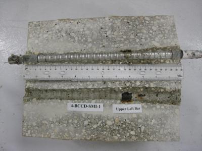
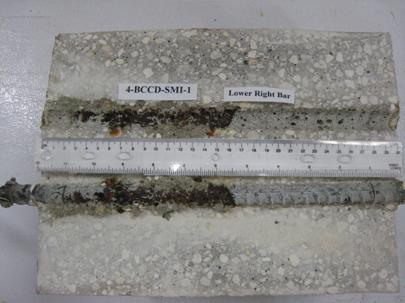
Figure 93. Photo. Lower R bar and bar trace of specimen 2-CCNB-316-2 subsequent to dissection.

Figure 94 and figure 95 show the typical appearance of top and bottom bars from specimen 4-BCCD-SMI-1. In the former case, corrosion has occurred locally at several of the 3-mm-diameter holes drilled through the cladding. Corrosion on the bottom BB was extensive, as seen in figure 95.

Figure 94. Photo. Top L bar and bar trace of specimen 4-BCCD-SMI-1 subsequent to dissection.

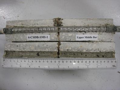
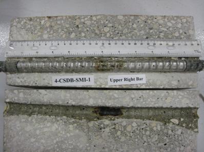
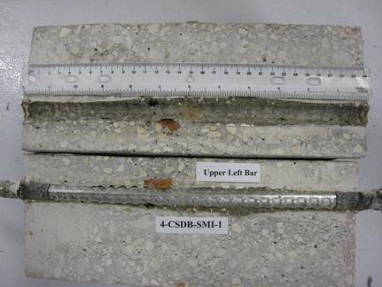
Figure 95. Photo. Lower R bar and bar trace of specimen 4-BCCD-SMI-1 subsequent to dissection.

Figure 96 to figure 98 show the appearance of the three top bars of specimen 4-CSDB-SMI-1 subsequent to dissection. Here, corrosion ranges from slight product staining (figure 98) to extensive staining at the crack base (figure 97). Corrosion at several of the 3-mm-diameter holes drilled through the cladding is also apparent away from the crack in figure 96 and figure 97.

Figure 96. Photo. Top C bar and bar trace of specimen 4-CSDB-SMI-1 subsequent to dissection.

Figure 97. Photo. Top R bar and bar trace of specimen 4-CSDB-SMI-1 subsequent to dissection.

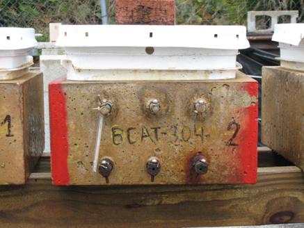
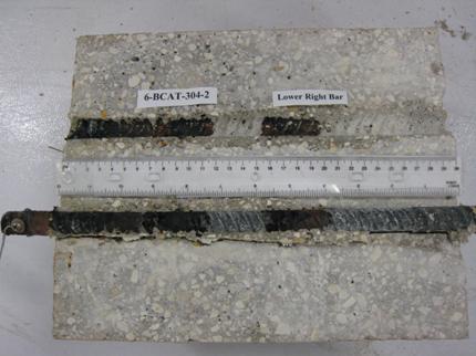
Figure 98. Photo. Top L bar and bar trace of specimen 4-CSDB-SMI-1 subsequent to dissection.

External appearance of specimen 6-BCAT-304-2 prior to dissection was characterized by corrosion product staining from each of the three bottom bars, as shown in figure 99. The red markings identify the specimen for removal.

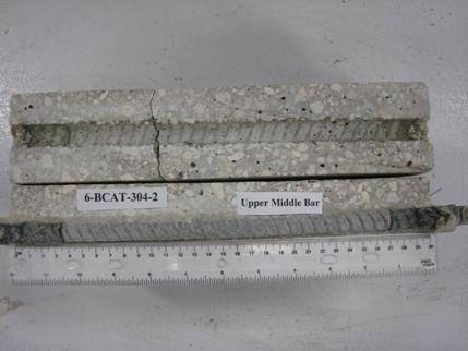
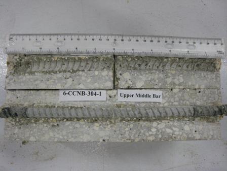
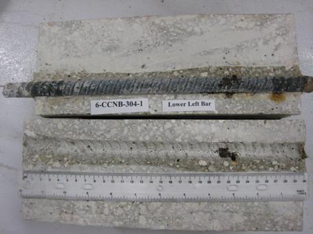
Figure 99. Photo. Specimen 6-BCAT-304-2 prior to dissection.

No corrosion was apparent on any of the top bars (figure 100) and ranged from nil to extensive on the bottom BB (figure 101). Likewise, no top bar corrosion was apparent on any of the three top bars of specimen 6-CCNB-304-1 (figure 102), and only minor corrosion was evident on the bottom BB (figure 103).

Figure 100. Photo. Top C bar and bar trace of specimen 6-BCAT-304-2 subsequent to dissection.

Figure 101. Photo. Lower right BB and bar trace of specimen 6-BCAT-304-2 subsequent to dissection.

Figure 102. Photo. Top C bar and bar trace of specimen 6-CCNB-304-1 subsequent to dissection.

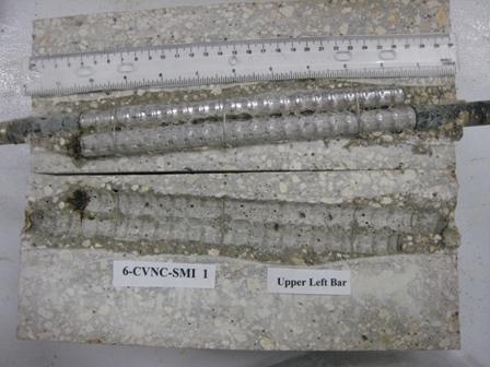
Figure 103. Photo. Lower left BB and bar trace of specimen 6-CCNB-304-1 subsequent to dissection.

Figure 104 shows a photograph of specimen 6-CVNC-SMI-1 after dissection where corrosion of the exposed carbon steel core is apparent (circled areas).

Figure 104. Photo. Top L bar pair and bar pair trace of specimen 6-CVNC-SMI-1 subsequent to dissection.

4.4.2 Dissection of MS Specimens

All but one of the improved performance MS specimens have been terminated and dissected. As indicated by figure 31 to figure 34, this was done well after corrosion had initiated. Table 63 reproduces T_i for these specimens from table 21 and also lists time at termination and time under test subsequent to T_i (propagation time, T_p).

Table 63. Listing of T_i, propagation time (T_p), and total time of testing for BB and improved performance bars in MS specimens.

In general, observations regarding the corrosion of bars from dissected MS specimens were in accord with those for SDS specimens. This is illustrated in figure 105 to figure 107, which show photographs of the three STD1-MMFX-2 specimens. For these and other specimens, the extent of corrosion tended to correspond to the length of T_p. Exceptions to this and examples of interest are discussed subsequently.

Figure 105. Photo. Top bar and bar trace for specimen MS-MMFX-2-A.

Figure 106. Photo. Top bar and bar trace for specimen MS-MMFX-2-B.

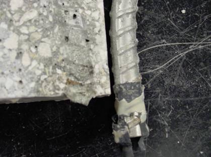
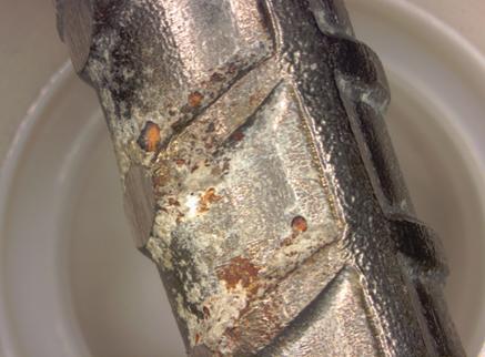
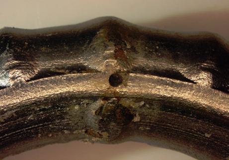
Figure 107. Photo. Top bar and bar trace for specimen MS-MMFX-2-C.

Figure 108 shows specimen MS-CBDB-MMFX-2-A after sectioning above the top bent bar. A small amount of corrosion product is apparent at what was the crack base and also near the bar ends.

Figure 108. Photo. Top bent bar trace in concrete for specimen MS-CBDB-MMFX-2-A.

Figure 109 shows the top bar from this specimen after its removal from the concrete.

Figure 109. Photo. Top bent bar from specimen MS-CBDB-MMFX-2-C after removal.

Corrosion was also disclosed on several of the high performance bars in MS specimens. Figure 110 provides one example where a small amount of corrosion products is apparent on the bar trace of specimen MS-CTNB-316-C (circled region) subsequent to dissection. The attack was beyond the footprint of the ponding bath and appeared to have resulted from crevice corrosion beneath the heat shrink sleeve.

Figure 110. Photo. Top bent bar from specimen MS-BTNB-316-C after removal.

Figure 111 shows similar corrosion that occurred on the top bent bar of specimen MS-CBNB-316-B.

Figure 111. Photo. Localized corrosion on the top bent bar from specimen MS-CBNB-316-B.

Lastly, figure 112 and figure 113 show corrosion at intentional 3-mm-diameter cladding defects on the top bent bar of specimen MS-CBDB-SMI-B. The defect in the first case was directly beneath the simulated crack, whereas the one in the second case was away from the crack in sound concrete.

Figure 112. Photo. Corrosion at an intentional clad defect on the top bent bar from specimen MS-CBDB-SMI-B.

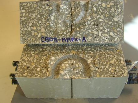
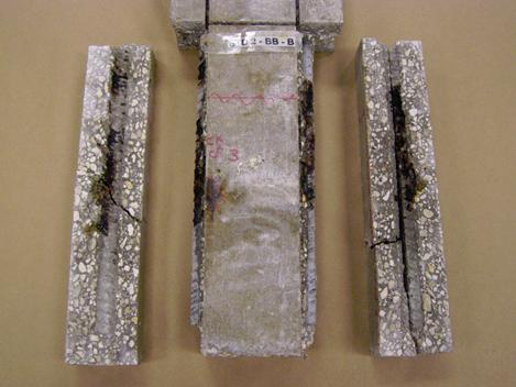
Figure 113. Photo. Corrosion at a second intentional clad defect on the top bent bar from specimen MS-CBDB-SMI-B.

4.4.3 Dissection of 3BTC Specimens

Only two 3BTC specimens, 3BTC-STD2-BB-B and 3BTC-STD2-2101-C, were dissected. Photographs of these are shown in figure 114 and figure 115. In both cases, concrete surface cracks were present in line with the longer bars. Corrosion is apparent upon the exposed bars, and corrosion products are visible along the rebar trace beginning about 200 mm above the specimen base.

Figure 114. Photo. Specimen 3BTC-STD2-BB-B after sectioning and opening along the two longer bars.

Figure 115. Photo. Specimen 3BTC-STD2-2101-C after sectioning and opening along the two longer bars.

4.5 Comparison of Results from Different Specimen Types

Table 64 lists the mean T_i for BB, 3Cr12, MMFX-2, and 2101 reinforced STD1-SDS and -MS specimens and the percent difference. Although caution must be exercised in placing too much emphasis on the differences because results for the MS specimens are based only on data for three bars of each type, T_i was still shorter for MS specimens than for SDS in the case of three of the four rebar types. This is in spite of the fact that the former were ponded with 3.0 wt percent NaCl and the latter with 15.0 wt percent NaCl. Apparently, the rate controlling steps for corrosion initiation were more rapid with the MS specimen design. In addition, comparison of the T_i results shows that for the SDS specimens, T_i (alloy)/T_i (BB) was in the approximate range of 2-4 for 3Cr12, MMFX-2, and 2101 (figure 28 and table 13) at 2 percent to 20 percent active. For the MS (figure 35 and figure 36), this ratio was near unity (within the range of expected experimental scatter). Thus, there was a lack of agreement between the two specimen types for ranking these reinforcements.

Table 64. Comparison of T_ivalues for STD-SDS and -MS specimens.

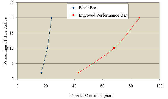
The STD2 mix design was common to both MS and 3BTC specimens, for which T_i (alloy)/T_i (BB) for MS MMFX-2 specimens was 3.4 to > 5.7 and 2.7 to > 4.8 for 2101 (table 23). For 3BTC specimens, these same ratios were 3.7-5.2 and 2.1-2.9 (table 44), indicating general mutual agreement. Data scatter precluded, including results for 3Cr12 in this analysis. For 3BTC STD3 specimens, the ratios were 1.2-3.1 for 3Cr12 and 0.9-3.2 forMMFX-2 (table 45) at 2 percent, 10 percent, and 20 percent active. For this class of specimens, experimental scatter for 2101 rebar specimens was sufficiently large that an analysis could not be performed. These results indicate that the T_i enhancement realized by these improved performance reinforcements was greater the higher the concrete quality. This happened because the greatest T_i (alloy)/T_i (BB) occurred for the STD2 mix design and least T_i (alloy)/T_i (BB) occurred for STD1. The STD1-MS specimens apparently provided too severe an exposure to reveal differences between these reinforcements. As noted in the previous section, macrocell current subsequent to T_i was greater for MS than SDS specimens, suggesting that the relative severity of the MS type specimen applies to the propagation as well as initiation phases.

4.6 Example Analysis

An example projection was made for T_i for a concrete member reinforced both with black steel and an improved performance CRR with properties within the range reported previously. In doing this, the C_T data in table 59 at 2 percent, 10 percent, and 20 percent active for BB and the average for 3Cr12 and MMFX-2 were employed (figure 81). These data are based upon exposures in STD1 concrete; however, for high quality concrete, greater enhancement of C_T for CRR relative to that for BB should result. In which case, an analysis based upon the previously listed choices should be conservative.

An effective Cl^- diffusion coefficient of 10^-12 m²/s, a concrete cover of 63 mm, and a surface [Cl^-] of 18 kg/m³ were assumed. The solution to Fick's second law (equation 3) was then employed to calculate T_i for each C_T. This yielded times-to-corrosion of 17 years and 43 years for BB and the CRR at 2 percent active and 24 years and 86 years at 20 percent active. Figure 116 provides a plot of these results.

Figure 116. Graph. Comparison of T_i at 2 percent to 20 percent activation for BB and an improved performance bar under conditions relevant to actual structures.

A limitation of this analysis is that it is based on mean values for D_e, x, and C_s, whereas, if fact, each of these parameters conforms to a distribution. Consequently, corrosion initiation at locations where D_e or x (or both) are less than the mean values and/or C_s is greater than the mean must be anticipated at lesser times than projected by figure 116. The calculation is based on one-dimensional diffusion; however, a lesser T_i should occur for bars at concrete corners where diffusion is in two dimensions.⁽²⁵⁾ Also, it is assumed that enhanced Cl^- transport along any concrete cracks is not significant. This shorter T_i compared to what is projected in figure 116 should be offset to some extent by the conservative choice for C_T in high performance concrete.

Time-to-corrosion calculations were not possible for the high performance reinforcements since T_iand C_T for these exceeded the exposure times and chloride concentrations that occurred. Certainly, C_T for these was greater than for the improved performance reinforcements, such that maintenance-free service life should extend well beyond the values in figure 116. In addition, the high performance bars provide greater confidence and margin for error.

Previous | Table of Contents | Next