• Federal Highway Administration >
• Publications >
• Research Publications >
• 09044 >
• Chap8.Cfm >
• Integrity of Infrastructure Materials and Structures

Publication Number: FHWA-HRT-09-044
Date: October 2009

Previous | Table of Contents | Next

CHAPTER 8. RESULTS AND DISCUSSION #2

TASK 2.1. LABORATORY TEST METHOD FOR PRODUCTION OF PROTECTIVE AND NONPROTECTIVE OXIDE LAYERS IN CHLORIDE ENVIRONMENTS

Weight Loss

To obtain values that could be compared, a corrosion value was computed, which consisted of a ratio between the weight loss and the exposed area. Time was not taken into account in that calculation. To compare data of a 15-cycle exposure to a 30–Cycle exposure, an average corrosion rate over a single cycle was computed by dividing the corrosion value by the number of cycles to which the coupon was exposed.

Calculations of the exposed surface area were made from the measurement of the four sides of the coupons. An average was performed on each set of two parallel sides and then multiplied with the edge areas summed to obtain the final exposed area. Some SAE1010 coupons had a hole made by the manufacturer for eventual hanging. The area of the hole and the edges were taken into account for the exposed area calculation.

Labeling the coupons was executed by beginning A606 coupon labels with "W" and SAE1010 coupon labels with "0." They were numbered consecutively from 01 to 96 for each kind of steel. The following two exposure charts, table 12 and table 13, provide information on the environments that were applied to the coupon identification numbers.

To assess the advantage of using weathering steel (A606) against carbon steel (SAE1010) in a particular environment, the corrosion value of A606 relative to SAE1010 can be calculated by computing the following:

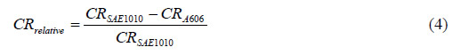
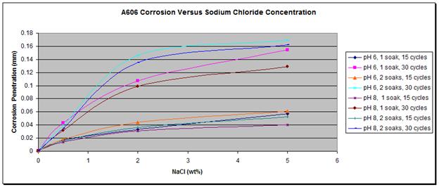
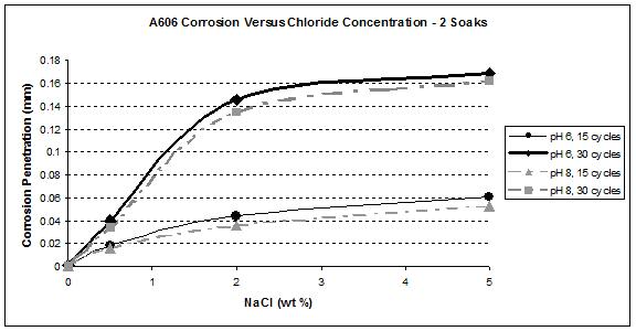
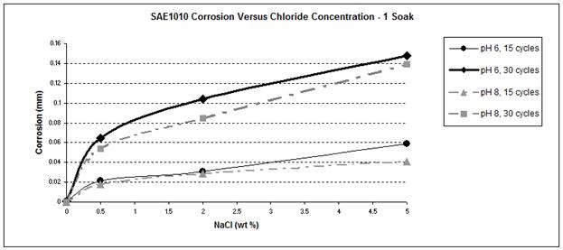
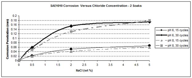
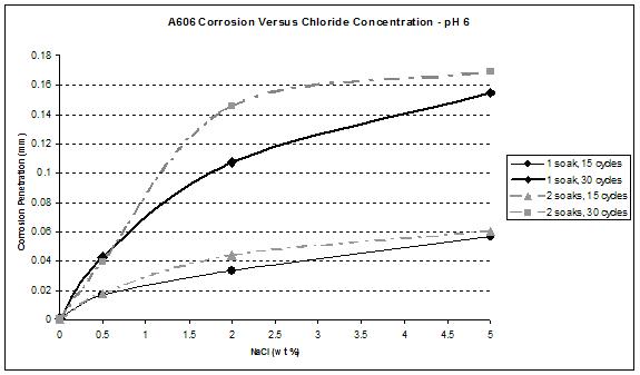
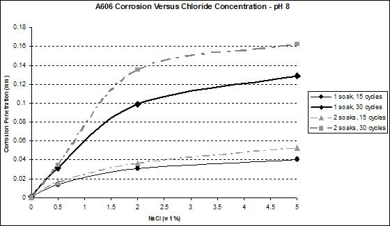
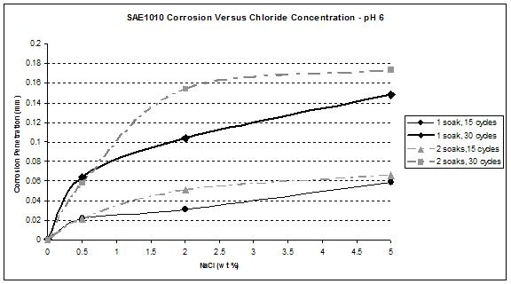
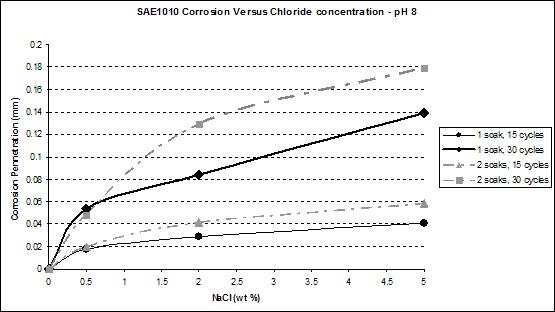
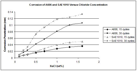
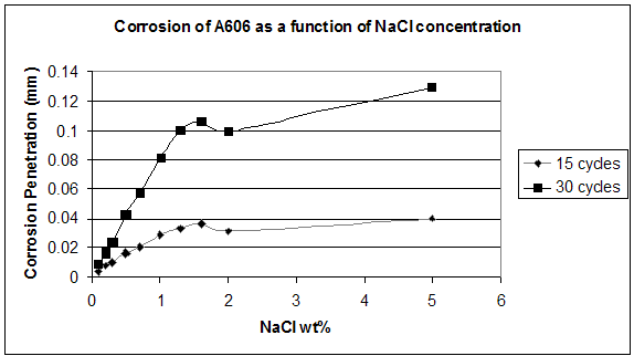
If the relative corrosion value was positive, weathering steel corroded less than the carbon steel during the exposure, meaning the patina impeded corrosion. Conversely, if the relative corrosion rate was negative, carbon steel performed better than weathering steel.

First Set Test

The complete set of data, which included individual specimen dimensions and weights, is available.⁽³¹⁾ An example calculation is given in the appendix for converting the data to units used in this report. Compilations of the data are in the following sections. The data are plotted and discussed as the average results of triplicate specimens unless stated otherwise.

Influence of Sodium Chloride

For both steel types, wetting times, or the pHs, a higher concentration of chloride led to a higher corrosion rate as shown in figure 31 and figure 32.

Figure 31. Graph. A606 corrosion as a function of the concentration of NaCl.

Figure 32. Graph. SAE1010 corrosion as a function of the concentration of NaCl.

During the corrosion process, Fe⁰ (metallic iron) was oxidized to Fe²⁺ in the solution. NaCl was present as the solvated ions, Na⁺ and Cl^-. When no salt was present on the surface of the steel, Fe²⁺ recombined with OH^— to form oxide and hydroxyoxide corrosion products (rust), as follows:

When salt was present, an intermediate product was involved and the following reaction occurred:

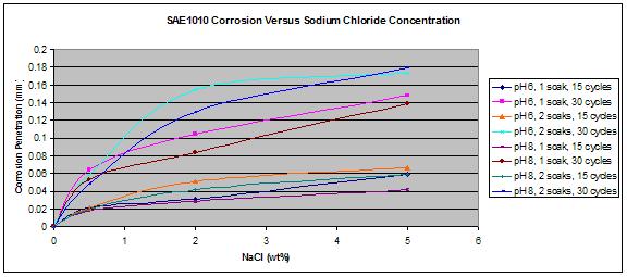
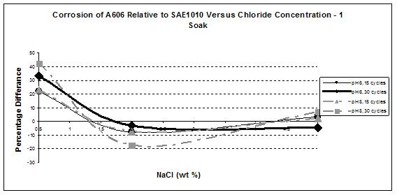
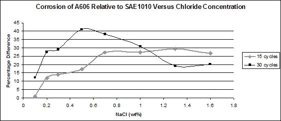
The most interesting feature was the weathering ability of A606 as a function of the chloride concentration. The results obtained from the first set test are summarized in figure 33, which shows the relative corrosion of A606 versus SAE1010. Figure 33 shows that while A606 developed its protective layer when using 0.5 percent NaCl at pH 6 and pH 8 (solutions 1-3 and 1-4), the two-soak exposure made it less protective. When using two soaks, the coupons were more exposed to NaCl (especially Cl- and water).

Figure 33. Graph. Relative corrosion between A606 and SAE1010.

Solutions 1-1 (zero percent NaCl and pH 6) and 1-2 (zero percent NaCl and pH 8) results are not shown in figure 33 because very little corrosion occurred due to the absence of chloride. Consequently, calculating the ratio (percentage) is problematic because the error factors are of the same magnitude as the results themselves. In addition, the ratios are not of interest for such low corrosion rates.

In figure 33, it is apparent that A606 performed very well in 0.5 percent NaCl and pH 6 (solution 1-3) and 0.5 percent NaCl and pH 8 (solution 1-4) for both one and two soaks, whereas poorer performances were found with the higher concentration NaCl solutions. Weathering steel was not as useful when high concentrations of NaCl were present. This result is consistent with suggestions of 0.1—1.0 percent maximum chloride concentrations for well-performing weathering steels.⁽³¹⁾ From these data, the interesting range of NaCl concentration, regarding weathering ability of A606, appears to be zero to 2 wt percent, justifying the choice of solutions for the second set test.

Influence of pH

Two different pH values were selected to study pH's influence on the corrosion of steel. Figure 34 through figure 37 present the corrosion values observed during the first set test. To clearly study pH's influence, the only parameter varied in each graph was the pH of the solution used during the soaking process. Data after 15 and 30 cycles are presented.

Figure 34 through figure 37 suggest that regardless of the type of steel, wetting time (one or two soaks/cycle), or exposure time, a lower pH yields a slightly higher corrosion rate. The variation of the pH does not appear to have a critical role in the early corrosion stage when the corrosion value is slightly affected.

Regarding the weathering ability of A606, figure 38 suggests that pH had a stronger effect with low NaCl. Conversely, at a high concentration of NaCl (5 percent) and a high number of cycles (30), pH had no effect.

Figure 34. Graph. A606 corrosion as a function of chloride concentration
during a one soak/cycle exposure.

Figure 35. Graph. A606 corrosion as a function of chloride concentration
during a two soak/cycle exposure.

Figure 36. Graph. SAE1010 corrosion as a function of chloride concentration
during a one soak/cycle experiment.

Figure 37. Graph. SAE 1010 corrosion as a function of chloride concentration
during a two soak/cycle experiment.

Figure 38. Graph. Relative corrosion versus NaCl concentration during
exposure to a one soak/cycle environment.

Influence of Wetting Time

Environments including one soak/cycle and two soaks/cycle were used to study the influence of the wetting time on the corrosion of the steels and the weathering ability of A606. Results are presented in figure 39 through figure 42.

Figure 39. Graph. A606 corrosion as a function of chloride concentration at pH 6.

Figure 40. Graph. A606 corrosion as a function of chloride concentration at pH 8.

Figure 41. Graph. SAE1010 corrosion as a function of chloride concentration at pH 6.

Figure 42. Graph. SAE1010 corrosion as a function of chloride concentration at pH 8.

Figure 41 and figure 42 show that the wetting time with high NaCl concentrations had a strong effect on SAE1010 as well as A606. Values with two soaks were much greater than those with one soak, especially for pH 8. Considering pH 6, corrosion values were becoming similar for the highest NaCl percentage. Increased wetting time and higher NaCl concentration had less influence on corrosion. A possible explanation is that at a high NaCl concentration, the oxide layer was saturated with NaCl, and the additional NaCl did not cause further change. However, at a lower pH of 6, corrosion increased, which suggests that a lower pH had a synergistic effect with NaCl to further saturate the oxide layer with chloride.

Second Set Test

The complete set of data, which includes individual specimen dimensions and weights, is available.₍₃₃₎ An example calculation is given in the appendix for converting the data to units used in this report. Compilations of the data are presented in figure 43 and figure 44. The data are plotted and discussed as the average results of triplicate specimens unless stated otherwise.

Figure 43. Graph. Corrosion of A606 and SAE1010 versus chloride
concentration for the second test set.

Figure 44. Graph. Relative corrosion versus chloride concentration.

Based on the first set of test results, an interesting range of chloride concentration was determined for the soaking solution, which was greater than zero and less than 2 percent NaCl. In these tests, only pH 8 was used with chloride concentration (0.1—1.6 percent NaCl), which was the only factor that was varied.

A606 performed well for 15 cycles. For a NaCl concentration greater than 0.5 wt percent, the weathering ability after 30 cycles seemed to decrease. This decrease is observed in figure 44 where the 30–Cycle data falls below that of the 15-cycle data. Issues might be encountered for longer exposure times because the corrosion rates for A606 increase for 30 cycles compared to 15 cycles.

XRD and Corrosion Rate

Several corrosion specimens were analyzed by XRD and correlated with their corrosion rates. The results are given in table 14 and discussed below. Table 14 presents the peaks and their intensities relative to the individual compound's major peak. These are semiquantitative percentages and do not intend to represent a quantitative rust composition. The results give indications concerning the composition of the rust and can be related to the results found in field studies. Additional XRD analyses are discussed in chapter 8.

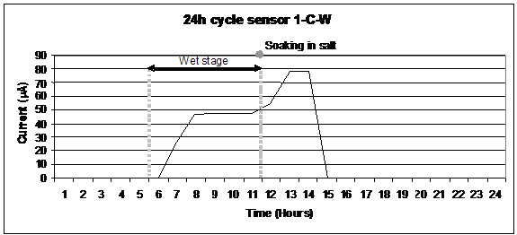
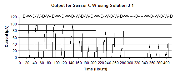
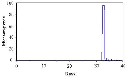
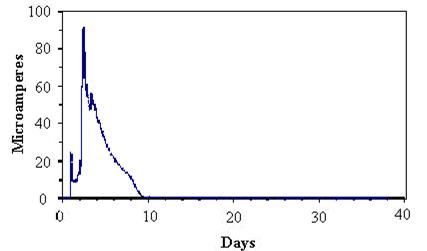
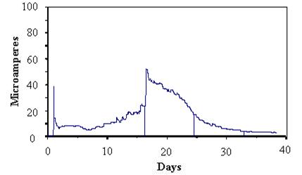
Weathering Steel—15–Cycle Exposure with Protective Patina

Coupon W67 was exposed to a solution of pH 8 containing 2 percent NaCl using one soak/cycle. Weight loss results showed that it developed a protective layer (see table 14).

The intensity peak was achieved by metallic iron (the substrate) at 44.7 degrees. The second peak of this pattern was at 21.7 degrees, which was the goethite strong peak. Its second strongest peak was present at 36.5 degrees. A small 27.8-degree peak indicated that lepidocrocite was present in the oxide layer.

Weathering Steel—30–Cycle Exposure with Protective Patina

Coupon W23 was exposed to a solution of pH 8 containing 0.5 percent NaCl using one soak/cycle. Weight loss results showed that it developed a protective layer (see table 14). The peak with the highest intensity at 21.7 degrees corresponded to the goethite peak, which was 81 percent of the protective patina. The second peak was also identified at 36.3 degrees. Peaks at 14.8 and 27.6 degrees corresponded to lepidocrocite. These smaller peaks indicated that there was little of this crystal phase in the oxide layer.

Weathering Steel—30–Cycle Exposure with Nonprotective Patina Exposed to High Chloride Concentration

Coupon W88 was exposed to 5 percent NaCl using one soak/cycle. Weight loss results showed that it did not develop a protective layer (see table 14).

Goethite was the main constituent of the oxide layer with peaks at 21.6 and 36.3 degrees. An iron peak was also present at 44.9 degrees and was likely due to metallic iron particles being undermined from the surface by corrosion or from scraping the coupon surface to remove the oxide for analysis. A small amount of maghemite was identified at 63.5 degrees. The first two maghemite peaks may have coalesced with the 36.3-degree peak of goethite.

Weathering Steel—30–Cycle Exposure with Nonprotective Patina Exposed to High Time of Wetness

Coupon W70 was exposed to 2 percent NaCl at pH 8 using two soaks/cycle (see table 14). Weight loss results showed that it did not develop a protective layer.

Goethite was identified by its main peak at 21.5 degrees. Its second peak was also present at 36.19 degrees. The relatively high intensity peak at 63.3 degrees indicated that a large fraction of maghemite was present in the oxide layer. The first two peaks of maghemite coalesced with the 36.3-degree peak of goethite.

Carbon Steel—30–Cycle Exposure with Nonprotective Patina Exposed to High Chloride Concentration

Coupon 070 was exposed to 2 percent NaCl at pH 8 using two soaks/cycle (see table 14). Weight loss results showed that it did not develop a protective layer. Goethite was the main constituent of the oxide layer. Maghemite was also observed at 63.6 degrees.

Analyses of Carbon and Weathering Steel Corrosion Products

XRD analyses were made on corrosion products obtained from additional specimens after completion of the cyclic tests. These are discussed in the next section.

Summary of XRD Analysis

The XRD results obtained from the coupons tested in the accelerated exposure chamber were in general agreement with the field study results given in table 14.(24) High wetting time developed maghemite and lepidocrocite, while high chloride developed maghemite and sometimes akaganeite. Goethite was present in every corrosion product whether it was protective or not. Thus, increasing the concentration of chloride, providing additional chloride exposure (a second soak), and increasing the wetting time all had the same effect in the laboratory as in field exposure. For example, specimens W67 and W23 exhibited low corrosion relative to W88, W70, and 070. The conditions of 2 percent NaCl (or lower) with a single soak represented low chloride and relatively drier conditions for W67 and W23. Conversely, conditions of 2 percent NaCl (or higher) with two soaks represented higher chloride and wetness exposures. The exposure chamber experiments produced results similar to those observed for steel in field exposure. Maghemite was found in almost all nonprotective corrosion products. One anomaly was the absence of akaganeite in the high chloride-soaked specimens, which may have been due to fresh water condensing humidity rinsing away chloride during the wet cycle portion. Generally, the laboratory tests were able to reproduce the conditions found during field exposure, especially with regard to high corrosion rate and maghemite correlation. Comparison of the laboratory and field exposures was not straightforward because the laboratory conditions could be controlled while the field conditions were dependent on natural (variable) environmental changes during the exposure.

TASK 2.2. CORROSION RATES OF ACCELERATED TEST SPECIMENS USING GALVANIC SENSORS

Reaction to Humidity and Salt Application

One of the successes of the sensor design described in the previous chapter was due to its very good response to humidity and NaCl. In figure 45, when the wet cycle began, the output immediately increased due to the completion of the current path, and the current was recorded by the data logger. The current remained stable during the time the metal was corroding; salt deposits and amorphous corrosion products were washed out by the ambient condensing humidity. Once the salt was applied, the current increased, responding to the corrosion rate of the material being exposed to a more aggressive environment. The wet stage occurred between the 6th and 12th hours, and soaking occurred at the 11th hour. After soaking the specimen, the dry cycle began, resulting in an increased current as the electrolyte layer dried. This increased the conductivity and infusion of oxygen through the thinner layer. When the drying was complete, the current dropped to zero. In the dry cycle, localized corrosion could occur as well as corrosion product crystallization and resizing of the crystallites.

Sensor output for the 15-cycle exposures is presented in figure 46. During the eighth cycle, the wet stage did not start because of an experimental chamber failure. The salt soaking was still performed, and each sensor responded the same way but with differing magnitudes. The outputs had the shape of a spike corresponding to the time needed for the salt solution to dry in the chamber. This unplanned event shows the reproducibility of the output for a given event over the whole sensor population, showing another success for the sensors. In the figure, D-W indicates approximate dry-wet periods.

Figure 45. Graph. Output for a Cu-A606 atmospheric corrosion sensor using soaking solution 3-1.

Figure 46. Graph. Output for Cu-A606 sensor during a 15-cycle test.

The output for the last three cycles after the weekend break was also interesting. Current readings dropped for each kind of steel, even more for A606. In the standard SAE J2334, the weekend break was optional. The reason why the corrosion rate decreased may be related to the crystallization time needed for the oxides to form. Oxides that constitute the protective layer needed to crystallize during the dry stage. If the dry stage was too short, the final crystallographic reformation was not complete, and consequently the protective layer was not completely formed. It is known that weathering steel requires dry and wet cycles to perform well, but the time required has not been characterized. If a corrosion performance test is to be developed further, drying time during weekends should be required or perhaps extended. Other data support this last statement. For the first set test (weight loss coupons), six weekend dry stages were performed, whereas for the second set test, only two weekend breaks were performed. By combining data obtained with the two exposure tests (see figure 40 and figure 43), figure 47 was created.

Figure 47. Graph. Corrosion of A606 versus NaCl concentration.

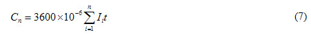
In figure 47, the corrosion value dropped between 1.6 and 2.0 wt percent NaCl. The data for 1.6 wt percent concentration was from the second set test, whereas the data for 2.0 wt percent concentration was from the first set test. The drop was due to the option of the experimental protocol that was not supposed to have a significant effect on the results according to standard SAE J-2334. The results show that drying time was an important factor when dealing with the corrosion of weathering steel. Weekend drying time should be included in the standard and should be a topic for additional study. The role of drying time was easily studied by cyclic coupon and sensor tests.

Corrosion Rate Determination

The sensors were intended to provide information about the corrosion rate of the material from which they were fabricated. To verify that the output of the sensors represents the actual corrosion rate in the same environment, the output of the sensors can be compared (see table 15) with the results obtained during the exposure of the coupons.

By integrating microamperes over the time, coulombs (i × t = C) are found, which are related to weight loss using Faraday's law. All microampere readings were averaged by the data logger over the sampling time of 1 hour (3,600 s). An example calculation is given in the appendix.

A coulomb is equal to amperes multiplied by seconds, as seen in equation 7.

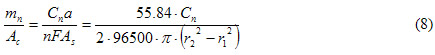
Note: G = gold; C = copper; W = A606; Q = SAE1010

To obtain a value that can be compared with the coupon data, equation 8 is used.

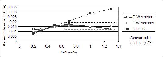
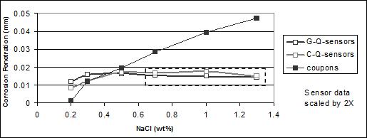
Plotting the sensor data and the coupons data gives figure 48 and figure 49. For both figures, the dashed boxes identify over-range sensor data.

Figure 48. Graph. Corrosion (weight loss) of A606 coupons and calculated mass-loss for
A606 sensors versus NaCl concentration for 15-cycle exposure.

Figure 49. Graph. Corrosion (weight loss) of SAE1010 coupons and calculated mass-loss
for SAE1010 sensors versus NaCl concentration for 15-cycle exposure.

For A606 steel (see figure 45), corrosion values calculated from the sensors were lower than those from the weight loss experiment (even after applying a 2X factor). However, the first three data points of sensors and coupons followed the same trend. The trend indicated that the more chlorides present in the solution, the higher the corrosion value. The last three (higher) concentrations reached a maximum corrosion value for the sensors. An explanation is that the output was off-scale, as can be seen on the sensors' output data. The amperes or coulombs obtained reached the maximum value (scale) that the data logger could record, indicated by a plateau with increasing chloride concentration. Consequently, those six data points (three for the G-W sensors and three for the C-W sensors) were invalid and should not be compared to weight loss data.

The same phenomena occurred for the SAE1010 sensors output. These sensors indicated that sensors made of SAE1010 were providing higher output values than (higher corrosion rate) that those made of A606. The higher rate was inferred by the coulomb values achieving maximum (plateau) values at lower chloride concentrations in figure 48 and figure 49 or higher values in table 15, especially for the copper cathode sensors. This result was reasonable due to the weathering ability of A606. Above a chloride concentration of 0.7 wt percent, the sensors produced an off-scale output that was invalid for quantitative comparisons. The first three sensor data points for both A606 and SAE1010 followed the trend of the coupon data where higher NaCl concentration indicated a higher corrosion value.

In general, sensors were able to indicate the corrosion rate of material exposed to the same environment, although a scale (proportionality) problem should have been considered. The sensors were sensitive to chloride concentration. A smaller active anode area or a wider range data logger is suggested for future studies. Table 15, figure 48, and figure 49 suggest that copper cathodes provide more consistent results than the gold cathodes.

RESULT OF TASK 2.3. PROTOTYPE CABLE CORROSION SENSORS

The main sources of moisture for cables are rainwater and condensation. These moistures are often mimicked by dilute Harrison solution for corrosion testing.(33) The solution contains ammonium sulfate and NaCl usually found in atmospherically deposited moisture.

Cable Sensor Response to Test Conditions

Figure 50 presents the sensor responses of dry specimens exposed to SAE J2334 cyclic conditions (except no soaking) followed by a experiencing a single soak in dilute (1/10 concentration) Harrison solution after 32 days and continuing the cycling without additional soaks. In each case, the sensors yielded little or no response until wetted by the dilute Harrison solution after 32 days. Each sensor showed a large increase in response after wetting. The responses observed were expected for wetted sensors. The specific nature of the response varied somewhat depending upon wetness saturation of the sensor within the specimen. In figure 50, the large response after wetting was followed by a large decrease corresponding to drying of the sensor. Subsequently, small responses that corresponded to the high humidity phase in the exposure chamber were observed every 24 hours.

Figure 50. Graph. Response of cable sensor before and after dilute Harrison solution.

Soaked

Figure 51 presents typical cable sensor responses of specimens soaked for 15 minutes in dilute (1/10 concentration) Harrison solution followed by equilibration under static conditions of 50 percent RH. Figure 52 presents the typical responses for similar tests for 100 percent RH. The responses showed that the more tightly wrapped specimens and those under the higher relative humidity maintained higher levels of current for longer times than loosely wrapped specimens or those under lower RH. These responses were consistent with corrosion that occurred in the presence of sufficient moisture.

Figure 51. Graph. Response of cable sensor during constant 50-percent RH
exposure after dilute Harrison solution.

Figure 52. Graph. Response of cable sensor during constant 100-percent RH exposure
after dilute Harrison solution.

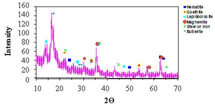
XRD Results for Cable Test Specimens

Table 16 and figure 53 show the XRD results for the corrosion products that were obtained from the cable specimen rods. The most notable difference compared to the coupon materials was the presence of butlerite. Butlerite is a ferrihydroxysulfate compound, and its formation is due to the presence of sulfate from the dilute Harrison solution used to wet the sensors

The bolded text, "0," represents SAE1010 material.
— Indicates that data was not found.
L = loose wrap.
T = tight wrap.
C = cyclic exposure.

Figure 53. Graph. XRD pattern of steel rods in cable sensor bundle after single soak in
dilute Harrison solution and exposure in cyclic chamber for 40 days.