Geosynthetic Reinforced Soil Integrated Bridge System Interim Implementation Guide

CHAPTER 4. DESIGN METHODOLOGY FOR GRS–IBS

4.1 OVERVIEW OF GRS–IBS DESIGN METHOD

During the past 30 years, GRS technology has been used to build walls, shallow foundations, culverts, bridge abutments, and rock fall barriers. The technology also has been used to stabilize slopes and repair roadways. This chapter focuses on the GRS design method used for GRS–IBS including an abutment and wing walls. While GRS technology can provide solutions in a variety of applications and under certain extreme conditions, the design method described in this manual provides a recipe for design of GRS–IBS with limitations on abutment heights, bridge spans, and design loads.

The design methods described in this chapter are appropriate for GRS structures (an abutment and wing walls) with a vertical or near vertical face and at a height that does not exceed 30 ft. Although the majority of bridges built with GRS–IBS have spans of less than 100 ft, spans of up to 140 ft have been constructed. While larger spans are possible, the bearing stress on the GRS abutment is limited to 4,000 lb/ft². The demands of longer spans on GRS–IBS are not fully understood at this time, and it is recommended that engineers limit bridge spans to approximately 140 ft until further research has been completed.

GRS–IBS abutment capacities are dependent on a combination of the strength of the fill material and the strength of the reinforcement when built in accordance with the two rules of GRS construction: (1) good compaction (95 percent of maximum dry unit weight, according to AASHTO T99) of high–quality granular fill and (2) closely spaced layers of reinforcement (12 inches or less). It is recommended that design or allowable bearing pressure be limited to 4,000 lb/ft².

For design pressures larger than 4,000 lb/ft², the performance criteria must be checked against the applicable stress–strain curve resulting from a performance test (discussed later in this chapter and in appendix B). The performance criteria for GRS–IBS consist of a tolerable vertical strain of 0.5 percent and lateral strain of 1 percent. A significant amount of research and practical experience has shown that GRS–IBS designed and constructed within the limits defined in this manual will produce safe, durable systems.

The design process starts with establishing the project requirements from which the preliminary geometry of GRS–IBS is determined. Once the geometry is defined, it is then evaluated against external and internal modes of failure. An iterative process is used to assess the geometry and make adjustments as necessary to facilitate construction and assure long–term performance. Economy should also be a consideration when evaluating each design alternative (e.g., deeper embedment versus larger footing).

A general and identifying feature of the GRS–IBS design is a mass built with alternating layers of compacted granular fill material and closely spaced reinforcement (less than or equal to 12 inches). In nearly all of the GRS masses built in the United States as full–scale experiments or as in–service structures, however, the design has been based on an 8–inch layered system. There are other features and principles common to a GRS mass. Most GRS walls have been built with dry–stacked concrete facing blocks and are flexible (in terms of global bending stiffness).

A GRS abutment is a type of gravity structure. Therefore, external stability should be evaluated for the direct sliding, bearing capacity, global stability, and overturning failure modes limiting this type of construction. However, because a GRS mass is relatively ductile and free of tensile strength, overturning about the toe, in a strict sense, is not a possible response to earth pressures at the back of the mass or loading on its top. Other attributes of GRS–IBS also tend to preclude overturning as a mode of failure. GRS–IBS consists of two abutments supporting an integrated superstructure that would function as a strut to resist overturning, and each GRS mass has a reinforced integration zone above its heel, also resisting the overturning mode of failure. Consequently, while direct sliding, bearing capacity, and global stability are evaluated in conventional ways, overturning is sometimes addressed by inspection and comparison to observations of past performance.

Observations of past performance show that the flexible, internally stabilized soil mass of GRS IBS construction, in combination with an RSF, results in more uniform stress distribution, resisting any applied vertical and lateral loads. Observations also show that, in addition to lack of overturning, the combination of vertical and lateral loads, as limited by analysis of direct sliding, bearing capacity, and global stability, does not cause excessive deformation at the face of the GRS mass or other undesirable performance.

While this combination of unique features and behavior eliminates the need to analyze overturning as a failure mode for completed GRS–IBS, the engineer may choose to analyze for overturning during an intermediate phase of construction with consideration for the time needed for an overturning mechanism to develop and the concurrent level of loading or for project configurations different from those described herein. For example, overturning may still be a viable failure mode for abutment wing walls constructed with GRS technology if they retain soil other than reinforced soil from the abutment or opposite wing wall (i.e., if they retain natural soil).

GRS is inherently internally stable because of the interaction between the soil and the reinforcement layers. The strength and stiffness of a GRS mass depends on the unique combination of compacted soil and reinforcement. The vertical capacity of the GRS abutment can be determined either empirically or analytically.

Empirically, the capacity is found using a stress–strain curve specific to the combination of the reinforcement type and granular fill material. If the designer uses a combination of the materials previously tested, then the appropriate stress–strain curve can be used for design. If the designer decides to change the materials from those already tested, then a performance test can be performed to obtain an applicable stress–strain curve for the empirical method. Guidelines on how to conduct a performance test are given in appendix B.

Alternatively, the designer can predict the ultimate vertical capacity of the GRS abutment by using an analytical equation. The equation is a function of reinforcement spacing, soil strength, and soil grain size. Note that the analytical method does not predict vertical deformation. A performance test is needed to adequately predict the deformation behavior of the GRS abutment. This design method is based on the results of many full–scale experiments and verified using case history performance data collected on several in–service GRS structures more than 20 years old.

The design of GRS–IBS is based on the following assumptions:

• The spacing of the reinforcement (12 inches or less) is a principal factor in the performance of GRS–IBS.

• A GRS mass is a composite material that is stabilized internally.

• Both the compacted granular fill and the reinforcement layers strain laterally together in response to vertical stress until the system approaches a failure condition.

• A GRS mass is not supported externally, and therefore, the facing system is not considered a structural element in design.

• Lateral earth pressure at the face of a GRS mass (i.e., thrust) is not significant, eliminating connection failure as a possible limit state.

• The facing elements of a GRS mass are frictionally connected to the geosynthetic reinforcement.

• Under the prescribed granular fill and reinforcement conditions, reinforcement creep is not a concern for the sustained loads. Therefore, individual reduction factors for reinforcement creep are not necessary. Creep can be accommodated safely within the factor of safety used for design.

As described in greater detail in subsequent sections of this manual, GRS–IBS design and construction processes follow from these basic assumptions and principles.

4.2 BASIC DESIGN STEPS FOR GRS–IBS

There are nine basic steps in the design of GRS–IBS (see figure 9). Note that the design philosophy illustrated in this section is Allowable Stress Design (ASD). It is FHWA policy that design for all Federal–aid funded projects be conducted using the AASHTO Load and Resistance Factor Design (LRFD) methodology. Guidelines to design GRS–IBS in an LRFD format are presented in appendix C. The LRFD format presented was normalized to produce the same results as the ASD method and does not represent a statistically based calibration that would be consistent with other AASHTO LRFD methods. After sufficient data is produced and collected as a result of this technology deployment and other efforts, a thorough statistical analysis will be performed to produce LRFD specifications for the design of GRS–IBS.

Figure 9. Chart. Steps for GRS–IBS design.

4.3 GRS–IBS DESIGN GUIDELINES

4.3.1 Step 1–Establish Project Requirements

The following parameters must be defined:

• Geometry of abutment and wing walls.

  • Height.
  • Length.
  • Batter (vertical or near vertical).
  • Wall placement with respect to ground conditions: back slope, toe slope.
  • Skew.
  • Grade.
  • Superelevation.

• Loading conditions.

  • Soil surcharge.
  • DL.
  • LL.
  • Seismic load.
  • Impact loads.
  • Loads from adjacent structures.

• Performance criteria.

  • Design format (e.g., ASD, LRFD).
  • Tolerable movements.
    • Vertical settlement.
    • Lateral displacements.
    • Differential settlement.
    • Angular distortion between abutments.
  • Design life.
  • Constraints.
    • Environmental.
    • Construction.

4.3.2 Step 2–Perform a Site Evaluation

To properly assess conditions at the site, a site visit must be conducted. During this visit, the following must be performed by the agency and/or its designer:

• Study the existing topography with respect to the proposed GRS–IBS.

• Check any existing structures/roads for problems to aid in the assessment and design.

• Conduct a subsurface investigation. Refer to AASHTO's Standard Practice for Conducting Geotechnical Subsurface Investigations for more information. Alternatively, refer to FHWA's Soils and Foundations Manual.( ⁶,⁷ )

  • Foundation soil properties (γ_f, Φ'_f, C'_f, C_u).
  • Groundwater conditions.

• Evaluate soil properties for the retained earth (γ_b, Φ_b, C'_b, C'_b).

• Evaluate soil properties for the reinforced backfill (γ_r, Φ_r , C_r, d_max). In addition to the basic soil properties, the maximum diameter of the granular backfill (d_max) is necessary to determine the ultimate capacity and required reinforcement strength. The gradation of the reinforced backfill is also important.

• Evaluate hydraulic conditions. This can be accomplished through consultation with a qualified hydrologist.

4.3.3 Step 3–Evaluate Project Feasibility

The feasibility of the project should be evaluated in terms of cost, logistics, technical requirements, and performance objectives. In particular, in the case of abutments for bridges constructed over water, the potential for scour, sedimentation, and/or channel instability must be evaluated in accordance with the policy and procedures of both FHWA and AASHTO. It is necessary to determine the potential for scour at all bridges constructed over water. If the abutment will be impacted by scour, additional design requirements are necessary (see chapter 6). These additional design requirements can be determined and implemented through a hydraulic and scour analysis of the site. Once the scour potential is determined, a countermeasure can be designed to protect the abutment against failure during a flood due to the scour that will occur at the toe of the abutment. A designed countermeasure will also protect the abutment from lateral channel migration that could undermine the foundation.

4.3.4 Step 4–Determine Layout of GRS–IBS

The layout of GRS–IBS is ultimately based on site conditions (e.g., desired road alignment, right of way, geotechnical issues, and hydraulic considerations). A survey should be conducted to determine the location of the GRS abutment and the layout. The layout of the abutment face wall needs to coincide with the wing walls because the system is built from the bottom up one course at a time. Both walls are built at the same time. Use the following steps to design the abutment:

1. Define the geometry of the abutment face wall and wing walls.

2. Layout the abutment with respect to the superstructure (skew, superelevation, grade).

   • The recommended minimum bearing width (b) for the superstructure is 2.5 ft for span lengths (L_span) greater than or equal to 25 ft, as shown in figure 10. For span lengths (L_span) less than 25 ft, the minimum bearing width is 2.0 ft.

3. Account for setback and clear space to calculate the elevation of the abutment face wall and the span length of the bridge.

   • The setback distance (a_b) between the back of the face and the beam seat should be the height of a standard CMU (nominally 8 inches) or more, as shown in figure 10.

   • The minimum clear space (d_e), defined as the distance from the top of the uppermost facing block to the bottom of the superstructure, should be 3 inches or 2 percent of the abutment height, whichever is greater (see figure 11). The gap is to ensure that the superstructure does not bear on the facing block due to an unforeseen event.

Figure 10. Photo. Bridge seat and setback distances.

Figure 11. Illustration. Clear space distance.

4. Determine the depth and volume of excavation necessary for construction. A GRS abutment is inherently stable and therefore can be built with a truncated base to reduce the excavation. Truncation also reduces the requirements for backfill and reinforcement.

   • For span lengths (L_span) greater than or equal to 25 ft, a minimum base width of the wall including the block face (B_total) of 6 ft should initially be chosen. For span lengths (L_span) less than 25 ft, a minimum base width of the wall including the block face (B_total) of 5 ft should initially be chosen. Whether a cut or fill situation, there should be a minimum base–to–height (B_total/H) ratio of 0.3. If GRS–IBS is to cross water, the base of the abutment should be placed at the calculated scour depth (see chapter 5).

   • Excavation of one–quarter the total width of the base of the abutment including the block face should be made at the base in front of the face of the wall to accommodate for construction of the RSF. The total width of the RSF should extend beyond the base of the GRS abutment by one – fourth the width of the base (see figure 12).

   • The depth of the excavation for the RSF (D_RSF) should equal one–quarter the total width of the base of the GRS abutment including the block face (see figure 12). Additional excavation may be necessary depending on the soil conditions (e.g., compressible soils) and should be determined by the engineer. In some situations, it may be beneficial to improve the ground beneath the RSF to reduce settlement of the bridge system.

   • Before designing and constructing an RSF, it is prudent to conduct a soil investigation of the existing foundation soil including applicable lab tests to determine the soil's properties, as discussed in section 4.3.2.

Figure 12. Illustration. RSF dimensions.

5. Select the length of reinforcement for the abutment. The minimum reinforcement length at the lowest level should extend the width of the base (B_total) and have a minimum base–to–height ratio (B/H) (not including the facing block) of 0.3. The minimum reinforcement length at the lowest level should extend the width of the base (B_total), with a minimum of 5–6 ft or a base–to –height ratio (B/H) of 0.3 (see previous step). Once the base length of the reinforcement is chosen, the reinforcement schedule should follow the cut slope, if applicable, up to a B/H ratio of 0.7. From there, the reinforcement length can get progressively longer in reinforcement zones (see figure 13). Not every layer will need to extend fully to the cut slope. The progressively longer lengths of reinforcement serve to improve the quality of construction and overall stability of the GRS abutment. The reinforcement zones also serve to provide a transition from the substructure to the superstructure. The exact details of the reinforcement zones, such as number of layers and length, are left to the designer. For cut slopes flatter than 1:1, reinforcement zones with lengths larger than 1H may not be necessary. The backfill between the reinforced zone and the cut slope or retained soil must be the same structural backfill as the reinforced fill and compacted to the same effort (see chapter 3). The reinforcement spacing should be no more than 12 inches at the wall face, in accordance with the two rules of GRS construction.

6. Add a bearing reinforcement zone underneath the bridge seat to support the increased loads due to the bridge (see figure 13). This bearing bed reinforcement serves as an embedded footing in the reinforced soil mass. The bearing bed reinforcement spacing directly underneath the beam seat should be, at a minimum, half the primary spacing (e.g., for an 8–inch primary spacing, the bearing bed reinforcement spacing will equal 4 inches). In general, the minimum length of the bearing bed reinforcement should be twice the setback plus the width of the bridge seat. The depth of the bearing reinforcement zone is determined based on internal stability design for required reinforcement strength (see section 4.4.7.3.1 4.4.7.3). At a minimum, there should be five bearing bed reinforcement layers (see figure 13).
   AMENDED May 24, 2012

Figure 13. Illustration. Reinforcement schedule for a GRS abutment.

7. Blend the reinforcement layers in the integration zone to create a smooth transition. The layers should extend to the cut slope, if applicable, with the exception of the top reinforcement layer, depending on the site. This top layer should extend beyond the cut slope to prevent moisture infiltration. The integration zone is part of the integrated approach of GRS–IBS (see figure 13). It is added behind the bridge superstructure to limit the development of a tension crack at the cut slope and reinforced soil interface and to blend the approach way on to the roadway to create a smooth transition. The number of reinforcement layers in the integration zone depends on the height of the superstructure, but each wrapped layer should be no more than 12 inches in height. Additional work is needed to integrate the substructure with the superstructure within the integration zone. This is described in chapter 7.

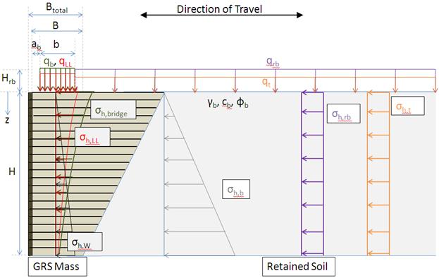
4.3.5 Step 5–Calculate Applicable Loads

The applicable external pressures and loads (permanent and transient) on the reinforced zone of the GRS abutment should be calculated. The most common pressures (which may be resolved into forces) on GRS–IBS for stability computations are depicted in figure 14.

Figure 14. Illustration. Vertical and lateral pressures on a GRS abutment.

The applicable pressures on a GRS abutment are as follows:

4.3.5.1 Lateral Pressures and Stresses

The lateral earth pressure can be calculated according to classical soil mechanics for active earth pressure. The active earth pressure coefficient (K_a) is calculated according to equation 1.

Where Φ is the friction angle of interest (for example, substitute Φ_b when calculating K_ab for the retained soil). The lateral stress distribution due to the weight of the GRS fill ( σ_h,W) is found using Rankine's active stress condition, shown in equation 2.

(2)

Where γ_r is the unit weight of the reinforced fill, z is the depth from the top of the wall, and K_ar is the coefficient of active earth pressure (equation 1) using the friction angle of the reinforced fill (Φ_r).

The lateral stress distributions due to the equivalent roadway LL surcharge (Σ_h,t) and structural backfill of the integrated approach ( Σ _h,rb) are found according to equation 3 and equation 4, respectively.

(3)

(4)

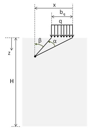
Where q_t is the equivalent roadway LL surcharge, q_rb is the surcharge due to structural backfill (road base), and K_ab is the coefficient of active earth pressure (equation 1) using the friction angle of the retained backfill (Φ_b). Note that equation 3 and equation 4 assume that the loading is continuous across the retained soil.

Where the loads are not continuous across the GRS abutment or retained soil, the lateral pressure is based on Boussinesq theory for load distribution through a soil mass for an area transmitting a uniform stress a distance x from the edge of the load (see figure 15 ).⁽⁸⁾ The actual pressure using this theory depends on the location of interest. For required reinforcement strength calculations, the location of interest is directly underneath the beam seat centerline (e.g., x = b_q/2 for the bridge DL).

Figure 15. Illustration. Boussinesq load distribution with depth for a strip load.

The lateral pressure due to surcharge loading (Σ_h,q) is calculated according to equation 5.

(5)

Where q is the surcharge pressure (e.g., q_b for the bridge surcharge), K_a is the coefficient of activeearth pressure (equation 1), and α and β are the angles shown in figure 15 , found using equation 6 and equation 7, respectively. Note that α and β must be input in radians in equation 5.

(6)

(7)

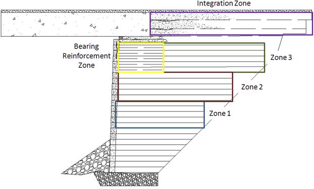
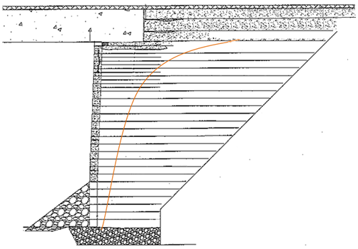
The lateral pressure in the GRS abutment due to the superstructure DL and LL will have a trend similar to that shown in figure 16 , where the stress is highest at the top of the GRS abutment and lowest at the base. Note that the bearing bed reinforcement underneath the beam seat helps to mitigate the increased vertical (and thus lateral) pressures in this location. In fact, the bearing bed reinforcement is recommended in the design of GRS abutments for this reason.

Figure 16. Illustration. Internal lateral stress in GRS abutment wall due to bridge loading.

Note that other load distributions are available besides Boussinesq. For example Westergaard is more applicable to a GRS mass than Boussinesq. However, it gives lower stresses than Boussinesq, and therefore, using Boussinesq will provide a more conservative estimate of stresses.

4.3.5.2 Dead Loads

4.3.5.2.1 Bridge: In a GRS–IBS design with adjacent concrete box beams, the bridge superstructure bears directly upon the GRS abutment. For superstructures with spread girders, a footing (which bears directly upon the GRS abutment) is necessary to ensure even load distribution on the GRS abutment. The equivalent DL design pressure on the abutment seat includes the dead loads due to the bridge beams, asphalt, overlay, guardrail, and any other applicable permanent loads related to the superstructure.

4.3.5.2.2 Road Base: Behind the bridge beams, road base is wrapped in geotextile (called the integrated approach). The wrapped face controls lateral load from the road base on the beam or abutment sill.

4.3.5.3 Live Loads

There are two applications of LL that affect the design of GRS–IBS: LL on the approach pavement and LL on the superstructure. Both of these live loads are defined by AASHTO and should be appropriately quantified by the design engineer.^{( 9 )}

4.3.5.3.1 LL on the Approach Pavement: An LL surcharge (q_t) is used to account for the vehicular load on the approach pavement leading up to the superstructure. This load consists of a uniform height (h_eq) of earth that produces an equivalent lateral effect on the abutment as the application of the vehicular LL specified for the superstructure. The equivalent height of earth is dependent on the abutment height and the orientation of the abutment with respect to the roadway (e.g., perpendicular). This load is used for both internal and external stability analyses.

4.3.5.3.2 LL on the Superstructure: The vehicular LL used for designing GRS–IBS is determined by applying the HL–93 LL model to the superstructure. This model consists of appropriately locating a design truck or design tandem in combination with a design lane load in each design lane of the bridge to create the maximum force effect at each abutment. The vehicular portion of the LL model is amplified for dynamic load allowance (impact). The governing LL is distributed to the abutment by multiplying by the number of design lanes and dividing by the bridge seat bearing area. This equivalent distributed LL pressure on the abutment seat (q_LL) can be determined using equation 8.

(8)

Where N_lanes is the number of design lanes on the bridge, b is the bridge seat bearing width (see figure 14), B_b is the width of the bridge, and (LL+IM)_total is the governing abutment reaction for the HL–93 LL model for one lane.

If the bridge seat bearing width is unknown and needs sizing, the LL from the superstructure should be quantified as a reaction (Q_LL) rather than a pressure (see equation 9).

(9)

4.3.5.4 Design Pressure

Adding LL on the superstructure and bridge DL per abutment will give the total load that the bridge seat must support. Dividing this total load by the area of the bridge seat will give the bearing pressure. For abutment applications, the bearing pressure should be targeted to around 4,000 lbs/ft². If this is exceeded, the width of the bridge seat should be increased. Although higher design pressures have been successfully applied to in–service GRS–IBS, this is not encouraged.⁽¹⁾

4.3.6 Step 6–Conduct an External Stability Analysis

The external stability of GRS–IBS is evaluated by looking at the following potential external failure mechanisms:

• Direct sliding (shown in figure 17 ).

• Bearing capacity (shown in figure 18 ).

• Global stability (shown in figure 19 ).

Figure 17. Illustration. External stability: direct sliding.

Figure 18. Illustration. External stability: bearing capacity.

Figure 19. Illustration. External stability: global stability.

4.3.6.1 Direct Sliding

The GRS abutment must resist translation, or direct sliding. The LL on the approach pavement (q_t)is assumed to act only over the retained backfill and not the reinforced soil mass. While the contribution of q_t (and q_LL) is ignored for both a wall and an abutment, the bridge load (q_b) has a stabilization effect against direct sliding when considering an abutment. Since the road base extends over the GRS abutment and the retained backfill, it acts to both stabilize and drive direct sliding. Contributions to both the driving force and to the resisting force from the road base must be taken into account because it is a permanent load.

The thrust forces behind the GRS abutment from the retained backfill (F_b), the road base (F_rb), and the roadway LL surcharge (F_t) are calculated using equation 10, equation 11, and equation 12.

(10)

(11)

(12)

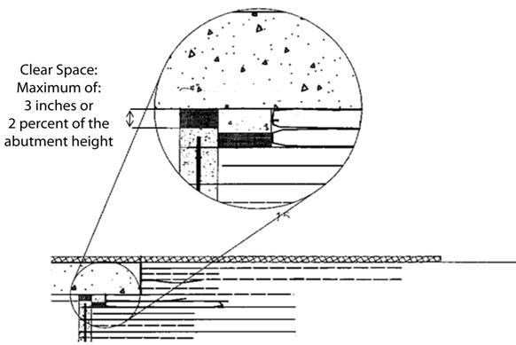
Where γ_bis the unit weight of the retained backfill, K_ab is the active earth pressure coefficient for the retained backfill (equation 1), H is the height of the wall including the clear space distance, q_rb is the road base DL, and q_t is the roadway LL.

The total driving force (F_n) is calculated by summing each thrust force previously calculated, as shown in equation 13.

(13)

The resisting force (R_n) is calculated according to equation 14.

(14)

Where W_t is the total resisting weight (calculated in equation 15), μ is the friction factor between the wall base and the foundation (taken as tan Φ_crit), and Φ_crit is the critical friction angle. Since the RSF is encapsulated with geotextile, sliding at the base of the GRS abutment will occur between soil and the geotextile reinforcement. The critical friction angle will therefore be the interface friction angle between the soil and reinforcement. The interface friction angle should be determined with an interface direct shear test for the particular combination of geosynthetic and reinforced fill material (ASTM D5321). If this information is not available for geotextiles and geogrids, assume that the friction factor is equal to ²/₃ times the tangent of the reinforced granularfill friction angle (μ = ²/₃tan(Φ_r)).

(15)

Where W is the weight of the GRS abutment (calculated in equation 16), q_b is the bridge DL, b is the width of the bridge load (measured along the direction of the roadway), q_rb is the road base DL, and b_rb,t is the width over the GRS abutment where the road base DL acts (see figure 14 ). The LL on the approach pavement and the superstructure are not included as resisting forces because they are transient loads.

(16)

Where γ_r is the unit weight of the reinforced fill, H is the height of the GRS abutment including the clear space distance, and B is the base width of the GRS abutment not including the wall facing. Direct sliding should also be checked at the interface between the RSF and the foundation soils.
AMENDED May 24, 2012

The factor of safety against direct sliding (FS_slide) is computed according to equation 17. The factor of safety must be greater than or equal to 1.5. If not, consider lengthening the reinforcement at the base.

(17)

4.3.6.2 Bearing Capacity

To prevent bearing failure, the vertical pressure at the base of the RSF must not exceed the allowable bearing capacity of the underlying soil foundation. The vertical pressure is a result of the weight of the GRS abutment, the weight of the RSF, the bridge seat load, the LL on the superstructure, and the LL on the approach pavement. The pressure at the base (σ_v,base,n) is calculated according to a Meyerhof–type distribution, shown in equation 18.⁽¹⁰⁾

(18)

Where ΣV is the total vertical load on the GRS abutment (calculated in equation 19), B_RSF is the width of the RSF, and e_B,n is the eccentricity of the resulting force at the base of the wall (calculated in equation 20).

(19)

Where W is the weight of the GRS abutment (equation 16), W_RSF is the weight of the RSF, W_face is the weight of the facing elements, q_tis the roadway LL, b_rb,t is the width of the traffic and road base load over the GRS abutment, q_rb is the road base surcharge, q_b is the bridge DL, b is the width of the bridge seat, and q_LL is the LL on the superstructure.

(20)

Where ΣM_D is the total driving moment, ΣM_R is the total resisting moment, and ΣV is the total vertical load (equation 19). The moments should be calculated about the bottom and center of the RSF for the specific layout of the GRS abutment. If e_B,n is negative, take e_B,n equal to zero for the term B_RSF–2e_B,n.

The bearing capacity of the foundation (q_n) can be found using equation 21.^{( 9 )}

(21)

Where c_f is the coehsion of the foundation soil, N_c, N_γ, and N_q are dimensionless bearing capacity coefficients as shown in table 4 , γ_f is the unit weight of the foundation soil, B' is the effective foundation width (equal to B_RSF–2e_B,n), and D_f is the depth of embedment. The friction angle in table 4 should be taken as the foundation's friction angle ( φ_f). If groundwater is present, modifications to equation 21 may be necessary and are provided by AASHTO.^{( 9 )}

Table 4. Bearing capacity factors.^{( 9 )}

The factor of safety against bearing failure (FS_bearing) is computed according to equation 22. The factor of safety must be greater than or equal to 2.5. If not, increase the width of the GRS abutment and RSF (by increasing the length of the reinforcements), replace the foundation soil with a more competent soil, or add embedment depth.

(22)

Beyond bearing capacity, consolidation settlement should be evaluated to ensure excessive deformations will not occur over the life of the bridge. Design considerations such as excavation and the RSF reduce the pressure on the foundation soil. Nevertheless, settlement of the foundation soil should be assessed as with any other spread footing according to FHWA guidance.^{( 7 )} Determining the criterion for tolerable foundation settlement is left up to the engineer.

A stress history analysis should be conducted to ascertain settlement and stability prediction. Answers to the following questions will provide insight on the stress history for an efficient design:

• Is the site bridge a replacement project built in the same location?

• What was the performance of the existing bridge?

• Were there any chronic maintenance issues associated with the existing structure?

• What was the combined weight of the abutment and superstructure within the footprint of the new bridge foundation? How does that stress compare with the stress of the new structure?

• Does the site involve an excavation equivalent to the weight of the new GRS–IBS?

• Can the new bridge be built behind the existing foundation?

4.3.6.3 Global Stability

Global stability is evaluated according to classical slope stability theory using either rotational or wedge analysis. To facilitate the global stability check, it is prudent to collect accurate soil property information. Standard slope stability computer programs can then be used to assess the global and compound stability of a GRS structure. The factor of safety for global stability should equal at least 1.5.

4.3.7 Step 7–Conduct Internal Stability Analysis

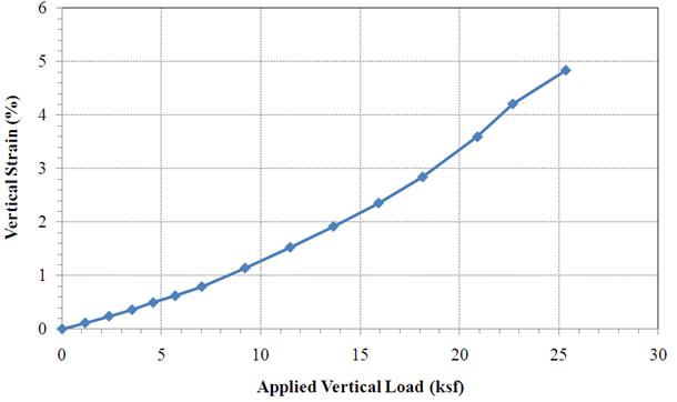
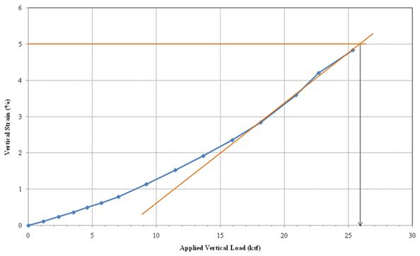
The internal stability analysis will vary slightly depending on the whether ASD or LRFD is the chosen design method. ASD is presented in this chapter. For guidance on LRFD, refer to appendix B C.
AMENDED May 24, 2012

4.3.7.1 Ultimate Capacity

The ultimate vertical capacity of a GRS abutment is found either empirically or analytically. It is recommended that the ultimate capacity be found empirically if possible. A performance test should be conducted to determine the ultimate capacity if the reinforced fill is different from those used in the performance tests reported in this guide (see appendix A). Testing will provide the most accurate results for the design. If a performance test cannot be performed, the analytical method can be used to determine the ultimate capacity.

4.3.7.1.1 Empirical Method: Empirically, the results of an applicable performance test using the same geosynthetic reinforcement and compacted granular backfill as planned for the site should be used. The ultimate vertical capacity in this case is defined as the stress at which the performance test mass strains 5 percent vertically. The ultimate vertical capacity is found in figure 20. For this performance test, the nominal capacity (q_ult,emp) is equal to 26 ksf for a vertical strain of 5 percent.

Figure 20. Graph. Design envelope for vertical capacity and strain at 8–inch reinforcement spacing.

Note that figure 20 represents the load–settlement performance of a GRS structure with reinforcement spaced at 8 inches, well–compacted AASHTO No. 89 fill material (having a friction angle of 48 degrees and no cohesion), and 4,800 lb/ft woven PP geosynthetic reinforcement. Other materials have also been tested and are shown in the synthesis report.^{( 1 )}

If the materials used are outside the recommendations provided in chapter 3, then a performance test must be performed to obtain the applicable stress–strain curve similar to figure 20. Guidance on setting up a performance experiment is given in appendix B. The total allowable pressure on the GRS abutment (V_{allow, emp}) is the ultimate capacity (q_ult,emp) divided by a factor of safety for capacity (FS_capacity) of 3.5, as shown in equation 23.

(23)

The applied vertical stress (V_applied), which is equal to the unfactored sum of the vertical pressures on the bridge bearing area, must be less than V_allow,emp (see equation 24). This includes the DL from the bridge (q_b) and the LL on the superstructure (q_LL). The DL due to the road base (q_rb) and the LL due to the approach pavement (q_t) are located behind the bearing area and are therefore not included in vertical capacity calculations related to the bridge superstructure.

(24)

4.3.7.1.2 Analytical Method: As an alternative, the load–carrying capacity of a GRS wall and abutment can also be evaluated using an analytical formula called the soil–geosynthetic composite capacity.^{( 11 )} The analytical formula was originally developed for GRS walls, but it is applicable to GRS abutments as well. Note that the analytical method assumes that the backfill satisfies the criteria outlined in chapter 3.

The ultimate load–carrying capacity (q_ult,an) of a GRS wall constructed with a granular backfill can be determined by the soil–geosynthetic composite capacity equation shown in equation 25.^{( 11 )}

(25)

Where S_v is the reinforcement spacing, d_max is the maximum grain size of the reinforced backfill, T_f is the ultimate strength of the reinforcement, and K_pr is the coefficient of passive earth pressure for the reinforced fill (calculated in equation 26).

(26)

Where Φ_r is the friction angle of the reinforced backfill. The friction angle should be determined from a large–scale direct shear device (ASTM D3080).

The total allowable pressure on the GRS abutment (V_allow,an) is the ultimate capacity found analytically (q_ult,an) divided by a factor of safety for capacity (FS_capacity) of 3.5 (see equation 27).

(27)

The applied vertical stress (V_applied), which is equal to the unfactored sum of the vertical pressures on the bridge bearing area, must be less than V_allow,an(see equation 28). This includes the DL from the bridge (q_b) and the equivalent LL on the bridge (q_LL). The DL due to the road base (q_rb) and the LL due to the approach pavement (q_t) are located behind the bearing area and are therefore not included in capacity calculations related to the bridge superstructure.

(28)

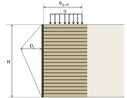
4.3.7.2 Deformations

The approach for determining vertical deformation involves empirically finding the strain from an applicable performance test curve. If the materials used are within the specifications given in chapter 3, then the curve shown in figure 20 can be used. Otherwise, a performance test must be conducted (see appendix B). The lateral strain is then determined analytically assuming the theory of zero volume change.^{( 12 )}

4.3.7.2.1 Vertical: The vertical strain of the GRS abutment is found from the intersection of the applied vertical stress due to the DL (q_b) and the performance test design envelope for vertical strain (see figure 20 ). The vertical strain should be limited to 0.5 percent unless the engineer decides to permit additional deformation. The vertical deformation, or settlement, of the GRS abutment is the vertical strain multiplied by the height of the wall or abutment. Because the GRS abutment is built with a granular fill, the majority of settlement within the GRS abutment will occur immediately after the placement of DL (q_b) and before the bridge is opened to traffic.

The settlement of the underlying foundation soils is determined separately using classic soil mechanics theory for immediate (elastic) and consolidation settlement. Factors such as excavation and the RSF should be taken into account, as the removal of overburden relieves stress on the foundation soil. Settlement of the foundation soil can be calculated using the FHWA Soils and Foundations Reference Manual.^{( 7 )}

4.3.7.2.2 Lateral: In response to a vertical load, the composite behavior of a properly constructed GRS mass is such that both the reinforcement and soil strain laterally together. This fact can be used to predict both the maximum lateral reinforcement strain and the maximum face deformation at a given load. The method conservatively assumes a zero volume change in the GRS abutment, which represents a worst–case scenario. The maximum lateral displacement of the abutment face wall can be estimated using equation 29.^{( 12 )} The lateral strain ( ε_L) is then found using equation 30 and should be limited to 1 percent.

(29)

(30)

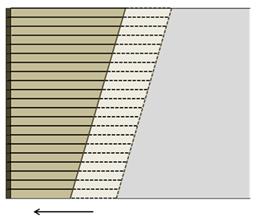
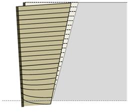
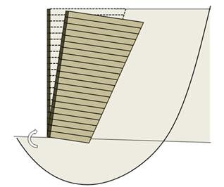
Where b_q,volis the width of the load along the top of the wall (including the setback), D_v is the verticalsettlement in the GRS abutment, H is the wall height including the clear space distance, and ε_Vis the vertical strain at the top of the wall. Note that equation 29 and equation 30 come from the assumptions of a triangular lateral deformation and a uniform vertical deformation (see figure 21 ). This assumption is based on observed deformation behavior of GRS. Also note that the location of the maximum lateral deformation depends on the loading and fill conditions, but the volume gained will still equal the volume lost. The maximum deformation of a GRS abutment often occurs in the top third of the abutment/wall.^{( 11–13 )}

Figure 21. Illustration. Lateral deformation of a GRS structure.

4.3.7.3 Required Reinforcement Strength

The required reinforcement strength in the direction perpendicular to the wall face (T_req) can be determined analytically by equation 31.^{( 11 )} The required reinforcement strength should be calculated at each layer of reinforcement to ensure adequate strength throughout the GRS abutment.

(31)

Where S_vis the reinforcement spacing, d_max is the maximum grain size of backfill, and σ_h is the total lateral stress within the GRS abutment at a given depth and location (calculated in equation 32).

(32)

Where σ_h,Wis the lateral earth pressure using Rankine's active stress condition (equation 2), σ_h,bridge,eq is the lateral pressure due to the equivalent bridge load (calculated in equation 33), σ_h,rb is the lateral pressure due to the road base (calculated in equation 34), and σ_h,t is the lateral pressure due to the roadway LL (calculated in equation 35). To simplify calculations, the approach LL and road base DL are extended across the abutment. The vertical components of these loads are then subtracted from the bridge DL and LL, giving an equivalent bridge load. The lateral stress due to the equivalent bridge load is then calculated according to Boussinesq theory. The location of interest to determine the maximum lateral pressure is directly underneath the centerline of the bridge bearing width.

(33)

(34)

(35)

Where q_b, q_rb, q_t, and q_LL are the bridge DL, road base DL, roadway LL, and bridge LL surcharges,respectively, and α_band β_bare the angles shown in figure 15, found using equation 36 and equation 37, respectively.

(36)

(37)

The required reinforcement strength (T_req) must satisfy two criteria: (1) it must be less than the allowable reinforcement strength (T_allow), and (2) it must be less than the strength at 2 percent reinforcement strain () in the direction perpendicular to the abutment wall face.
AMENDED May 24, 2012

In design, a minimum value of the ultimate reinforcement strength (T_allow) is needed to ensure adequate ductility and satisfactory long–term performance. In addition, it is prudent to specify the resistance required at the working load () to ensure satisfactory performance under the in–service condition.

For abutments, a minimum ultimate tensile strength (T_f) of 4,800 lb/ft is required. The allowablereinforcement strength (T_allow) is found by applying a factor of safety for reinforcement strength (FS_reinf) of 3.5 to the ultimate strength (see equation 38). The required reinforcement strength (T_req) must be less than T_allow.

(38)

Since geosynthetic reinforcements of similar strength can have rather different load–deformation relationships depending on the manufacturing process and the polymer used, it is important that T_req be less than the strength at 2 percent reinforcement strain. The strength of the reinforcement at 2 percent () is often given by the geosynthetic manufacturer. If T_reqis greater than , a different geosynthetic must be chosen, the ultimate strength must be increased, or the reinforcement spacing must be decreased.

While the strength of the reinforcement can theoretically vary along the height of the GRS abutment, it is recommended that only one strength of reinforcement be used throughout the entire abutment. This simplifies the construction process and avoids placement errors for the reinforcement.

4.3.7.3.1 Depth of Bearing Bed Reinforcement: The required reinforcement strength (T_req) is found at each 8–inch primary spacing layer. If T_req is greater than the allowable reinforcement strength (T_allow) or the strength at 2 percent strain (), then the reinforcement spacing must be reduced to 4 inches to the depth at which T_req is less than T_allow or .This depth is termed the bearing reinforcement bed. The minimum required depth is five courses of block.

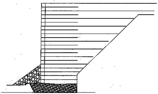
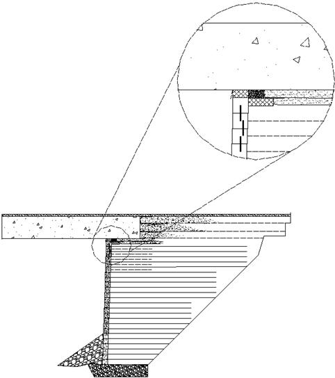
To check that 4–inch spacing for the bearing reinforcement bed is adequate, calculate the required reinforcement strength again for this new spacing in the top layers to ensure that T_req is less than T_allow and for all layers throughout the GRS abutment.

4.3.8 Step 8–Implement Design Details

figure 22 and figure 23 are typical cross sections of a GRS wall (or wing wall) and an abutment face wall and illustrate design details that will be discussed in this section.

Courtesy of Defiance County , OH
Figure 22. Illustration. Typical cross section of a GRS wing wall.

Courtesy of Defiance County , OH
Figure 23. Illustration. Typical cross section of a GRS abutment face wall.

In the case of an abutment, finalize the design layout for ease of construction, drainage, and other considerations that might affect the performance, serviceability, or efficiency of design. The following are some GRS design implications and related details for consideration:

• Conduct a hydraulic analysis in accordance with all appropriate regulatory and policy guidance (see chapter 5). Consult a licensed hydraulic engineer if necessary.

• Ensure that the face of the abutment (which includes the parapet) is wide enough to accommodate the installation of guardrails (see figure 24 ). The additional width should be enough to allow the guardrail to lay down. This lay–down length is approximately 4 ft. Steel rail posts should be used because wooden posts are nearly impossible to drive into the GRS mass.

Figure 24. Photo. Guardrail lay–down distance.

• Consider a core of native soil in the center of the abutment face and two adjacent wing walls to minimize excavation (see figure 25 ). The wing walls can be truncated like the abutment. Extend the wing walls sufficiently into the cut slope to prevent erosion caused by undermining or piping. This should be a minimum of two facing–block lengths.

Figure 25. Photo. GRS abutment and wing walls built around core of native soil

• Determine whether to build wing walls with either a full face or a stepped face that leads into the cut slope. The decision depends on several factors related to the height of the abutment, grade of fill slope (which is usually at 2:1), and time and materials. For abutments less than 12 ft in height, a full face is probably most efficient as it is the easiest to construct. However, for abutments greater than 12 ft, it might be more efficient to design a stepped –face wall (i.e., tiered wall) that leads into the cut slope. Stepped walls use less material but require additional labor in building the second foundation to support the extended stepped wall. In either case, all facing blocks should be supported on well–compacted structural fill.

• Include channel drains along the wings walls to facilitate runoff. The drain path should not be located directly against the wall face. Armor the drain path with a strip of geotextile beneath a layer of channel rock. Grade in compacted native soil against the wing walls with a slope leading to the drainage path.

• GRS–IBS has been used for bridges with skew, superelevation, and grade without problems or serviceability issues.

  • For a skewed bridge, it is important to maintain the minimum bearing area of 2.5 ft along the length of the abutment face wall.

  • For a bridge with superelevation, it is important to ensure that the minimum number of bearing bed reinforcement layers beneath the beam seat (calculated in step 7) are installed across the length of the abutment face.

  • At this time, there are no special considerations for opposing GRS abutments that support a bridge on a grade.

• Contain the GRS integrated approach fill by wrapping the geotextile layers adjacent to the beam ends to prevent lateral spreading (see chapter 7). Extend the reinforcement layers at the approach back onto the road, as indicated in figure 23.

• Avoid any abrupt transition of soil type from the roadway to the bridge. While the RSF and abutment should use a reinforcement with a minimum ultimate strength of 4,800 lb/ft, a lighter geosynthetic of about 2,400 lb/ft could be used for the integrated approach. However, it is recommended that only one strength of reinforcement be used on site to simplify the construction process and avoid placement errors.

• Plan ahead to avoid trenching, and account for the possible installation of utilities.

• Locate and plan to accommodate existing and potential future utilities.

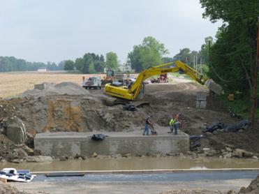
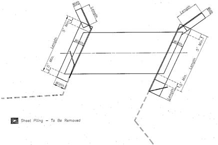
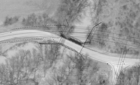
4.3.9 Step 9–Finalize Material Quantities and Layout

To develop the reinforcement schedule, choose a reinforcement length that makes use of the entire roll of the reinforcement material. Reinforcement material is usually 12– to 18–ft wide. For example, the width of a PP geosynthetic roll is 12 ft, and the base of a GRS wall is 6 ft including the width of the wall face. The roll can be cut in half by a chainsaw, and a 6–ft–wide roll can be used to build the base of the wall. The remaining 6–ft–wide rolls can be used for secondary or intermediate layers of reinforcement in the walls.

Draw the layout to scale to avoid errors in the calculation of quantities. Add 10 percent to the estimate of all materials. When using CMU, use the exact dimensions of 7⁵/₈ inches by 7⁵/₈ inches by 15⁵/₈ inches and buy both corner and face blocks.

Building GRS abutments vertically without a batter eliminates the need to trim blocks. This will make it more difficult to hide lateral movement and may give an illusion of instability when the structure is, in fact, stable. Use only high–quality, well–graded gravel, as specified in chapter 3.

4.4 DESIGN EXAMPLE: BOWMAN ROAD BRIDGE , DEFIANCE COUNTY , OH

Construction of Bowman Road Bridge was completed in October 2005 by a Defiance County, OH,construction crew. This project represents the initial deployment of GRS–IBS. The structure was chosen for a design example because it demonstrates many of the variables that can be accommodated by GRS–IBS technology and illustrates the versatility of the construction method.

4.4.1 Step 1–Establish Project Requirements

GRS–IBS was used for the Bowman Road Bridge project. The project included an abutment and a wing wall on each side of the bridge. A top view of the proposed project is shown in figure 26. figure 27 is an aerial view of the site with the proposed bridge superimposed.

Figure 26. Illustration. Top view of Bowman Road Bridge showing the bridge, abutments, and wing walls.

Figure 27. Illustration. Aerial view of the existing site with the planned Bowman Road Bridge superimposed.

Schematics of the proposed abutments are shown in figure 28 and figure 29 . The project requirements are as follows:

• Geometry.

  • Wall height (H_abut): 15.25 ft.

  • Abutment length (L_abut): 43.6 ft.

  • Bridge width (B_b): 34 ft.

  • Batter ( ω ): 2 degrees.

  • Wall placement with respect to ground conditions (back slope, toe slope): None.

  • Skew (S_k): 24 degrees.

  • Grade (G): 0.006 ft/ft.

  • Superelevation (S_e): 7.6 degrees.

• Loading Conditions.

  • Soil surcharge: Road base will be placed behind the bridge beam to create a smooth transition.

  • DL: DL includes the weight of the bridge beam along with any corresponding components.

  • LL: LL includes traffic and truck loads which are simulated as a surcharge.

  • Seismic load: Seismic effects are negligible in this area.

  • Impact loads: No impact loads are considered.

  • Loads from adjacent structures: Not applicable.

• Performance Criteria.

  • Design code: ASD.

  • Tolerable movements.

    • Vertical settlement: Vertical strain ( ε_V) is limited to 0.5 percent.

    • Lateral displacements: Lateral strain (ε_L) is limited to 1 percent.

  • Design life: 100 years.

  • Constraints.

    • Environmental: None.

    • Construction: Sheet piling from the existing bridge remains in place, reducing the need for two wing walls in the IBS. Only one wing wall is required.

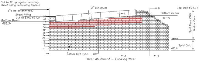
Figure 28. Illustration. Schematic of the west abutment for Bowman Road Bridge.

Figure 29. Illustration. Schematic of the east abutment for Bowman Road Bridge.

4.4.2 Step 2–Site Evaluation

The previous bridge at the site was replaced because it was functionally obsolete and structurally deficient. The previous bridge did not experience any problems related to settlement or excessive deformations due to the site conditions. However, a sheet pile wall was installed to protect the stone wall abutments from erosion. The site evaluation determined that the existing sheet piling should remain in place to support the stream bank. This eliminated the need for wing walls on one side adjacent to the old bridge.

The replacement structure required realignment to meet current road design standards for roadway safety because the location had been prone to accidents. The new Bowman Road Bridge crosses Powell Creek. The proposed location of the new abutments adjacent to the old bridge was not expected to cause any problems with the stream flow.

A hydraulic analysis confirmed that the existing bridge did not have any appreciable potential scour. Therefore, an RSF with appropriate scour countermeasures (in this case, riprap) was used.

A subsurface evaluation was conducted by performing standard penetration tests (SPTs) near the site. The physical characteristics of the soil were determined through index tests taken on split spoon samples. The foundation soil at the site was an overconsolidated clay (with intermediate layers of sandy silt and gravels) with N–values greater than 50 blows per ft at the elevation of the bottom of the abutment (determined from figure 28 and figure 29). Local experts indicated the clay had historically been preloaded with a nearly 1–mi–thick sheet of ice. The clay in this region is also known to be fat and sticky when wet. The bearing capacity of the stiff clay had not been a problem in past projects in the area.

The N–value of the foundation soil can be correlated into an undrained shear strength using published guidance.^{( 8 )} For blow counts greater than 30 blows per ft, the unconfined compressive strength is greater than 8,000 lb/ft². The undrained shear strength is therefore estimated as at least 4,000 lb/ft². The design properties for the foundation soil are shown in table 5 .The retained backfill is composed of the same material as the foundation soil.

Table 5. Foundation and retained backfill soil properties.

The road base was a granular fill material that was brought to the site. For the Bowman Road Bridge project, the properties of the road base are given in table 6.

Table 6. Road base soil properties.

The reinforced fill for the GRS abutment was a select granular fill (AASHTO No. 89 stone). Testing was performed on this fill to determine the c and Φproperties. The properties of this fill are provided in table 7.

Table 7. Reinforced fill properties.

4.4.3 Step 3–Evaluate Project Feasibility

As mentioned in step 2, scour was not a significant concern for this bridge. The project was therefore considered feasible for this site. Scour protection was added as a precaution. The riprap was sized for 8.8–10.2 ft/s to create a scour protection apron adjacent to and in front of the abutment face and wing walls. Prior to placement, a 5– to 8–ft–wide strip of geotextile reinforcement between the face of the RSF and the riprap was pinned under the first course of facing blocks to secure it in place. The purpose of the geotextile reinforcement was to create a barrier to mitigate loss of soil beneath the riprap.

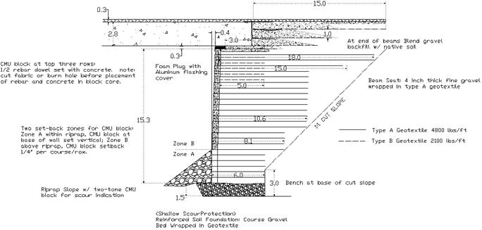
4.4.4 Step 4–Determine Layout of GRS–IBS

1. Define the geometry of the abutment face wall and wing walls: See step 1.

2. Layout the abutment with respect to the superstructure: See figure 29. The distance between the abutment faces was 72 ft. Therefore, since the length of the bridge was greater than 25 ft, the minimum bearing width (b) for the superstructure was 2.5 ft. A bearing width of 4 ft, however, had been chosen for this bridge.

3. Account for setback and clear space: The bridge seat had a setback of 8 inches from the edge of the wall. The clear space was 4 inches, which was greater than 2 percent of the wall height.

4. Determine the depth and volume of excavation necessary for construction:

   • A base width of the wall including the block face of 6 ft was chosen for this abutment since the span length was greater than 25 ft and 0.3H was less than the 6–ft minimum. Subtracting the wall face width (7.625 inches), the reinforcement length at the base of the wall was 5.4 ft. This equates to a B/H ratio of 0.35, which is greater than the minimum B/H ratio of 0.3.

   • Excavation of 1.5 ft (one–quarter the width, including the block face) was made at the base in front of the face of the wall to accommodate for construction of the RSF. The total width of the RSF was therefore 7.5 ft.

   • The depth of the excavation for the RSF was equal to one–quarter the width of the base including the block face–1.5 ft (see figure 12 ).

5. Select the length of reinforcement for the abutment: The reinforcement length at the base of the wall was equal to 6 ft (or 5.4 ft not including the reinforcement necessary for the frictional connection). The reinforcement lengths up the wall were chosen based on the cut slope angle and an optimization of the width of the reinforcement rolls. The reinforcement schedule is shown in figure 30.

Figure 30. Illustration. Reinforcement schedule and RSF dimensions for Bowman Road Bridge.

6. Add a bearing reinforcement zone underneath the bridge seat: The primary reinforcement spacing was 8 inches at the wall face. The spacing of the bearing reinforcement bed was 4 inches, half of the primary spacing. The length of the bearing reinforcement bed was 5 ft. The depth of the bearing reinforcement bed would be determined when the internal stability analysis was conducted (step 7). At a minimum, however, there would be five intermediate layers between the primary reinforcement layers (at 8–inch spacing) in the bearing reinforcement zone (see figure 12 ).

7. Blend the reinforcement layers in the integration zone to create a smooth transition: Additional work was needed to integrate the substructure with the superstructure within the integration zone at the approach (see figure 12 ). There were three layers of wrapped geotextile reinforcement spaced at 0.9 ft. This is described in chapter 7.

4.4.5 Step 5–Calculate Loads

The applicable surcharges and loads associated with the structure were a combination of vertical and lateral components. The vertical components include the surcharges due to the DL (superstructure and road base from the integrated approach) and the LL (superstructure and roadway), along with the weight of the GRS abutment. The lateral earth pressure due to the retained backfill, shown in table 8, were also considered. Lateral loads resulting from the DL and LL were calculated separately during the external and internal stability calculations performed in step 6 and step 7.

Table 8. Loads and surcharges for Bowman Road Bridge.

Note that the weight of the GRS abutment was calculated with B equal to the shortest reinforcement layer not including the width of the wall face. This is a conservative assumption to simplify hand calculations. Several software programs are available that can account for the varying shape due to different reinforcement lengths along the height of the abutment. The weight of the facing blocks (W_face) is the weight of an individual CMU block (42 lb) divided by the length of theblock (15.625 inches), multiplied by the total number of blocks in a single column (24 in this case).

4.4.6 Step 6–Conduct an External Stability Analysis

4.4.6.1 Direct Sliding

The driving forces on the GRS abutment include the lateral forces due to the retained backfill, the road base, and the traffic surcharge.

The force due to the backfill is calculated in equation 39.

(39)

The lateral force due to the road base and traffic surcharges are calculated in equation 40 and equation 41, respectively.

(40)

(41)

The total driving force (F_n) is then calculated in equation 42.

(42)

The resisting force (R_n) is calculated according to equation 14. The total resisting weight (W_t) includes the weight of GRS plus the weight of the bridge beam plus the weight of the road base over the GRS abutment. Since the live loads are not permanent, they cannot be counted as a resisting force. Total resisting weight (W_t) is calculated in equation 43.

(43)

The friction force (μ) is equal to tan Φ_crit. The interface friction angle between the reinforced fill and the geotextile was measured at 39 degrees by conducting an interface direct shear test. The resisting force (R_n) calculation is shown in equation 44.

(44)

The factor of safety against direct sliding (FS_slide) is calculated in equation 45 to make sure it is greater than 1.5.

(45)

4.4.6.2 Bearing Capacity

Before calculating the applied vertical bearing pressure, the eccentricity of the resulting force at the base of the wall must first be calculated using equation 20.

The moments are calculated around the center of the base of the RSF. The driving moments (calculated as a counterclockwise moment) include the lateral force due to the retained backfill, the road base DL, and the roadway LL. The calculation is shown in equation 46.

(46)

The resisting moments (calculated as a clockwise moment) include the vertical force due to the bridge and road base DLs and the bridge and roadway LLs. The weight of the GRS abutment is also included as a resisting moment. This calculation is shown in equation 47.

(47)

The total vertical load is equal to the sum of the weight of the GRS abutment, the weight of the RSF, and the load due to the DLs (bridge and road base) and LLs (bridge and roadway). This calculation is shown in equation 48.

(48)

Thus, the eccentricity of the resulting force at the base of the RSF is calculated in equation 49.

(49)

The applied vertical pressure is then calculated in equation 50.

(50)

The bearing capacity is calculated in equation 51. The bearing capacity factors N_c, N_γ, and N_q were found using table 4 for the foundation friction angle of 0 degrees.

(51)

The factor of safety against bearing capacity failure is calculated in equation 52 to make sure it is greater than 2.5.

(52)

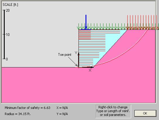
4.4.6.3 Global Stability

Global and compound stability was checked using the software program ReSSA. Figure 31 is a screenshot of the global stability failure mode. The factor of safety was found to equal 6.6, much greater than the minimum requirement of 1.5. Global and compound stability were satisfied.

Figure 31. Screenshot. ReSSA results for global stability for Bowman Road Bridge.

4.4.7 Step 7–Conduct Internal Stability Analysis

4.4.7.1 Ultimate Capacity

The ultimate capacity of a GRS abutment can be determined using two different methods: empirical or analytical.

4.4.6.1.1 Empirical Method: The empirical method uses the load test results of a performance test on a GRS composite material identical (or very similar) to that used in the field. The ultimate capacity is found empirically as the stress at 5 percent vertical strain from the stress–strain curve shown in figure 32. For this curve, the ultimate capacity (q_ult,emp) is 26 ksf.

Figure 32. Graph. Stress–strain curve for Bowman Road Bridge showing ultimate capacity.

The total allowable pressure on the GRS abutment (V_allow,emp) is the ultimate capacity (q_ult) divided by a factor of safety for capacity (FS_capacity) of 3.5, as shown in equation 53.

(53)

The applied vertical stress (V_applied), which is equal to the unfactored sum of the vertical pressures on the bridge bearing area, must be less than V_allow,emp. This includes the DL from the bridge (q_b) and the LL due to the notional HL–93 load model (q_LL), as shown in equation 54.

(54)

4.4.7.1.2 Analytical Method: Alternatively, the ultimate capacity can be found analytically for a granular backfill. S_v is equal to 8 inches, d_max is equal to 0.5 inches,T_f is equal to 4800 lb/ft, and Φ_r is equal to 48 degrees ( see table 7 ). Although the spacing under the bridge bearing area was 4 inches, 8 inches was chosen in equation 55 to be conservative.

(55)

The passive earth pressure for the reinforced fill was determined with equation 56.

(56)

The total allowable pressure on the GRS abutment (V_allow,an) is the ultimate capacity (q_ult,an) divided by a factor of safety for capacity (FS_capacity) of 3.5, as shown in equation 57.

(57)

The applied vertical stress (V_applied), which is equal to the unfactored sum of the vertical pressures on the bridge bearing area, must be less than V_allow. This includes the DL from the bridge (q_b) and the LL due to trucks (q_LL). Applied vertical stress is calculated in equation 58.

(58)

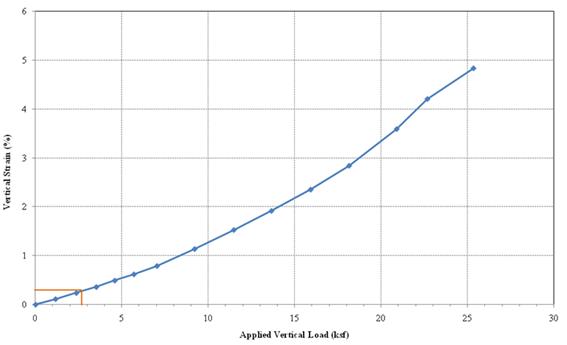
4.4.7.2 Deformations

4.4.7.2.1 Vertical: The vertical strain is estimated by using figure 32 , as illustrated in figure 33 for the bridge DL (q_b) of 2,600 psf. The vertical strain is therefore about 0.3 percent–under the tolerable limit of 0.5 percent. The road base surcharge is not included since it does not act over the same location.

Figure 33. Graph. Vertical strain for Bowman Road Bridge.

The vertical deformation is the product of the vertical strain and the height of the GRS abutment (including the clear space distance), as shown in equation 59.

(59)

4.4.7.2.2 Lateral: The lateral strain and deformation are found in equation 60 and equation 61.

(60)

(61)

4.4.7.3 Required Reinforcement Strength

The strength of the reinforcement used at Bowman Road Bridge was 4,800 lb/ft. Applying a factor of safety of 3.5, the allowable reinforcement strength is 1,371 lb/ft. According to the manufacturer, is equal to 1,370 lb/ft.

The maximum required reinforcement strength is found as a function of depth, as shown in equation 62.

(62)

The lateral stress (σ_h) is a combination of the lateral stresses due to the road base DL (σ_h,rb), the roadway LL (σ_h,t), the GRS reinforced soil (σ_h,W), and an equivalent bridge load (σ_h,bridge,eq). To simplify calculations, the roadway LL and road base DL can be extended across the abutment. The vertical components of these loads are then subtracted from the bridge DL and LL, giving an equivalent bridge load. The lateral stresses due to the equivalent bridge load are then calculated according to Boussinesq theory. The lateral stress is calculated for each depth of interest (each layer of reinforcement). All lateral stresses are calculated and shown in table 9.

Table 9. Depth of bearing bed reinforcement calculations.

Distance from top of wall	Equivalent Bridge Load			Road Base DL and Roadway LL		GRS Fill	Total	Required Strength	Ultimate Check	2 Percent Check
z (ft)	α	β	σh,bridge,eq (psf)	σh,rb (psf)	σh,t (psf)	σh,W (psf)	σh,total (psf)	Treq (lb/ft)	Treq > Tallow	Treq >
0.7	2.50	–1.25	482	57	44	11	593	1024	NO	NO
1.3	1.97	–0.98	449	57	44	22	572	987	NO	NO
2.0	1.57	–0.79	400	57	44	32	533	920	NO	NO
2.7	1.29	–0.64	350	57	44	43	493	852	NO	NO
3.3	1.08	–0.54	305	57	44	54	460	794	NO	NO
4.0	0.93	–0.46	269	57	44	65	434	749	NO	NO
4.7	0.81	–0.40	239	57	44	76	415	716	NO	NO
5.3	0.72	–0.36	214	57	44	86	401	692	NO	NO
6.0	0.64	–0.32	193	57	44	97	391	675	NO	NO
6.7	0.58	–0.29	176	57	44	108	385	664	NO	NO
7.3	0.53	–0.27	162	57	44	119	381	658	NO	NO
8.0	0.49	–0.24	149	57	44	130	380	655	NO	NO
8.7	0.45	–0.23	139	57	44	140	380	655	NO	NO
9.3	0.42	–0.21	129	57	44	151	381	658	NO	NO
10.0	0.39	–0.20	121	57	44	162	384	663	NO	NO
10.7	0.37	–0.19	114	57	44	173	388	669	NO	NO
11.3	0.35	–0.17	108	57	44	184	392	676	NO	NO
12.0	0.33	–0.17	102	57	44	195	397	685	NO	NO
12.7	0.31	–0.16	97	57	44	205	403	695	NO	NO
13.3	0.30	–0.15	92	57	44	216	409	705	NO	NO
14.0	0.28	–0.14	88	57	44	227	415	717	NO	NO
14.7	0.27	–0.14	84	57	44	238	422	729	NO	NO

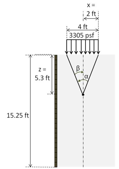
An example calculation for the required reinforcement strength at a depth (z) of 5.3 ft, or the eighth reinforcement layer from the top (see figure 34 ), is presented here. First, the lateral pressure is found in equation 63. Remember, the location of interest is directly under the centerline of the bridge load (where x = 0.5b =0.5(4ft) = 2 ft).

(63)

The calculation of each aspect of the lateral pressure is shown in equation 64 through equation 67.

(64)

(65)

(66)

(67)

The values for α and β are found in equation 68 and equation 69.

(68)

(69)

Figure 34. Illustration. Lateral pressure due to the bridge load.

Based on table 9, the required reinforcement strength does not exceed the allowable strength or the strength at 2 percent at any reinforcement layer. Therefore, no bearing bed reinforcement is needed; however, the minimum requirement is that the bearing bed reinforcement should extend through five courses of blocks. In actuality, six courses of block were chosen to extend the bearing reinforcement bed in this case (to a depth of 4 ft below the top of the wall). This was chosen to be conservative since this was the first bridge built with GRS technology.

Applying 4–inch spacing to the top six courses of blocks and 8–inch spacing for the remaining height of the wall, the required reinforcement strength was found (see table 10 ). The maximum required reinforcement is 716 lb/ft, which is less than the factored reinforcement strength of 1,371 lb/ft and the reinforcement strength at 2 percent. There should, therefore, be no issues with reinforcement strength in the abutment.

Table 10. Required reinforcement along height of wall.

4.4.8 Step 8–Implement Design Details

All design details were considered. Since it was a skewed bridge, the bearing area of 3 ft was maintained along the length of the face wall. The bearing bed reinforcement schedule was also maintained across the abutment face due to the superelevation, as shown in figure 35.

Figure 35. Illustration. Secondary reinforcement for superelevation at Bowman Road Bridge.

4.4.9 Step 9–Finalize Material Quantities and Layout

The amount of reinforcement necessary is based on the reinforcement schedule. Reinforcement material came in 12– to 18–ft–wide rolls. The number of facing blocks was determined from the height and length of the abutment and wing walls. The amount of backfill required was determined in a similar fashion. Once final quantities are established, it is a good rule of thumb to order at least 10 percent more to account for unforeseen conditions.