U.S. Department of Transportation
Federal Highway Administration
1200 New Jersey Avenue, SE
Washington, DC 20590
202-366-4000
Federal Highway Administration Research and Technology
Coordinating, Developing, and Delivering Highway Transportation Innovations
 |
| This report is an archived publication and may contain dated technical, contact, and link information |
|
Publication Number: N/A
Date: November 1996 |
The purpose of these measurements is to determine absolute DGPS signal strengths at various distances from eight different Coast Guard beacons transmitting DGPS signals and to measure signal strength at various distances from an FAA beacon located in the same frequency band. Four of the measured DGPS beacons are located along the Gulf Coast and four are on the West Coast. The measured FAA beacon is located in Bennett, Colorado east of Denver. Each of the transmitters are described in Table 1. Results of the measurements are used to provide model inputs and to compare results to actual model predictions.
Table 1. Beacon Characteristics
| Location | Freq (kHz) | Antenna | Tran Rate BPS | Latitude (N) | Longitude (W) |
| Aransas Pass, TX | 304 | PA90B | 100 | 27 50 18 | 97 03 33 |
| English Turn, LA | 293 | PA90B | 200 | 29 52 44 | 89 56 31 |
| Galveston, TX | 296 | PA90B | 100 | 29 19 45 | 94 44 10 |
| Mobile Point, AL | 300 | 150 ft Tower | 100 | 30 13 38 | 88 01 24 |
| Pigeon Point, CA | 287 | PA90B | 100 | 37 10 55 | 122 23 35 |
| Point Blunt, CA | 310 | PA90B | 200 | 37 51 12 | 122 25 04 |
| Cape Mendocino, CA | 292 | PA90B | 100 | 40 26 29 | 124 23 56 |
| Fort Stevens, OR | 287 | PA90B | 100 | 46 12 18 | 123 57 21 |
| Bennett, CO | 321 | Unknown | N/A | 39 47 31 | 104 26 03 |
 |
|
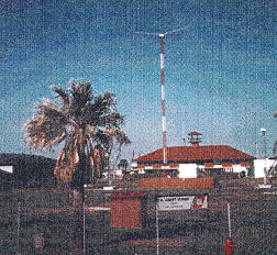
Figure 1. Transmitter at Aransas Pass.
|
Measurements in the southern region were conducted by driving along the Gulf between Corpus Christi, Texas and Mobile Alabama. On the first day, the measurement van was driven to the Coast Guard station at Aransas Pass (Figure 1). Starting approximately 17 km from the transmitter, signal strength measurements (304 kHz band only) were performed as the measurement vehicle was driven along the southwest edge of the bay, through Corpus Christi, circling around the bay to the north. On the second day, measurements were conducted between Corpus Christi, Texas and Lafayette, Louisiana while traveling along highways 77, 59, and Interstate 10. All four Coast Guard transmitters were monitored continuously (except for a short break as the vehicle came in close proximity to the Galveston site). The vehicle was driven to the town of Galveston via Highway 6 and then transported by ferry across the bay. Measurements resumed on the opposite shore.
 |
|
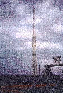
Figure 2. Transmitter at Mobile Point.
|
Data were acquired to within five km of the Galveston transmitter. Shortly after reaching the opposite side of the bay (approximately 6:00 p.m.), the sun set. For the remainder of the distance between Galveston and Lafayette, data were acquired at nighttime. On the third day, measurements were conducted continuously on all four Gulf State transmitters as the vehicle traveled between Lafayette, Louisiana and Mobile, Alabama along Interstate 10. En route, the measurement vehicle came within 11 km of the English Turn transmitter. On the fourth day, measurements were conducted near the Mobile Point transmitter (300 kHz band only) as the vehicle was driven to the transmitter site from the west side of the bay. Data were acquired to within 10 km of the transmitter (Figure 2).
On the West Coast, signal strength measurements were conducted on each of the four DGPS transmitters by driving the following routes: Data were acquired on the Cape Mendocino signal while driving north from Santa Rosa, California along Highway 101 within 12 km of the transmitter and continuing north to Crescent City, California. From there, the measurement vehicle was driven along Highway 199 to Grants Pass, Oregon. Cape Mendocino is located approximately halfway between Santa Rosa and Grants Pass along Highway 1. Data were acquired on the Fort Stevens signal starting at a distance of 10 km from the transmitter on Highway 30, traveling along the Columbia River east to The Dalles. Both nighttime and daytime data were acquired on the Pigeon Point and Point Blunt transmitters. Pigeon Point is located approximately 45 km north of Santa Cruz along Highway 1, and Point Blunt is located on Angel Island in the San Francisco Bay. Nighttime data were acquired by driving south from Willits, California along Highway 101 to the Golden Gate Bridge and continuing along Highway 1 to Santa Cruz. Daytime data were acquired by starting 6 km south of the Pigeon Point transmitter traveling south to Santa Cruz, across the coastal mountains on Highway 17, north on the eastern border of the bay along Interstate 680, east along Interstate 80, over the Sierra Nevada mountains, and past Reno, Nevada.
Data on the FAA beacon at Bennett, Colorado were acquired on two different routes. The first route started at the transmitter traveling west along Interstate 70 over the Rocky Mountains to Grand Junction, Colorado. The second route started at the transmitter traveling west along Interstate 70 to Interstate 25 and then north to approximately 50 km north of Cheyenne, Wyoming. The primary reason for measuring the signal strength on the FAA beacon is to examine the propagation characteristics through the Rocky Mountains west of Denver.
Figure 3. Block diagram of measurement system.
The measurement system (seen in Figure 3) consists of a receiving antenna, low pass filter, amplifier, spectrum analyzer, GPS/DR receiver, and a computer. The antenna was calibrated for antenna correction factors at 2 kHz intervals between 285 kHz and 325 kHz (see Appendix D). The low pass filter serves to filter out all frequencies above 400 kHz, particularly the AM broadcast bands. The computer is used to control the spectrum analyzer, download raw data, gather GPS information, and perform various computations. The overall gain of the system (including cables) is approximately 24 dB. The noise figure of the system is 9.6 dB, giving a sensitivity of 7.85 dB µV / m for a bandwidth of 300 Hz (see Appendix C). The GPS receiver has a dead reckoning system such that, if satellite lock is lost, the proper coordinate information is maintained.
The computer controls the acquisition of data using GPIB and RS232 commands sent to the spectrum analyzer and GPS receiver, respectively. Data are also downloaded via GPIB and RS232. Two types of data are acquired: noise and DGPS signal strength.
Prior to acquiring data on the DGPS signal, the power of the noise is determined by making measurements 500 Hz offset from the DGPS carrier frequency. The purpose of measuring noise is simply to determine if the signal, as a whole, can be detected against the noise background. The purpose is not to determine environmental noise, even though, in many cases, this may be the primary source of noise. Three types of measurement procedures were used: type 1 in the Gulf States, type 2 for Cape Mendocino, and type 3 for all the remaining beacons along the West Coast and Colorado. Type 1 measurements use a 500 Hz span and sweep across the frequencies in that span. To avoid measuring power from the adjacent DGPS signal itself, the resolution bandwidth is set to 30 Hz. A single sweep is performed in 360 ms, after which the mean, the standard deviation, and the peak noise power are determined from 601 data points evenly spaced across the 500 Hz bandwidth. Type 2 measurements use a zero span with a 300 Hz bandwidth and sweep in time. A single sweep is performed in 700 ms, after which the mean, the standard deviation, and the peak noise power are determined from 601 data points evenly spaced in time. In addition, 50 samples evenly spaced across the 601 data points are stored in the record header. Because the filters on the HP8563 spectrum analyzer have a gentle roll-off and the measured signals are only 500 Hz offset from the location of the noise measurements, this technique results in an upward bias due to the contribution of power by the adjacent signal. Therefore, the measurement technique was changed to a type 3 noise measurement shortly after completing data acquisition on the Cape Mendocino beacon. The type 3 measurement uses a 200 Hz span with a 10 Hz bandwidth and sweeps across the frequency band. A single sweep is performed in 350 ms, after which the mean, the standard deviation, and the peak noise power are determined from 601 data points evenly spaced in time. In addition, 50 samples evenly spaced across the 601 data points are stored in the record header. For all three techniques, there is an upward bias when the noise measurements are conducted in close physical proximity to the transmitter because the signal can significantly contribute to the power received within the bandwidth. This, again, is because the filters in the HP8563 spectrum analyzer have a gentle roll-off and the measured signals are only 500 Hz offset from the location of the noise measurements.
The DGPS signal strength is measured by performing 50 separate sweeps of a 500 Hz span spaced between one to five seconds apart. After each sweep, the signal power is determined and recorded in the data file. For a type 1 acquisition, the peak power over the entire span is determined and recorded. For a type 2 and 3 acquisition, the power is determined at the DGPS center frequency. The latter is believed to be better since the former may cause a slight upward bias from spurious noise spikes. Based on the antenna correction factor and the known frequency, the signal field strength is calculated as described in Appendices A and B. With each sweep, a data string from the GPS / DR system is downloaded and placed in the file to mark the location of the acquisition. Each of the four parameters (frequency, power, field strength, and GPS coordinate string) are recorded for each of the 50 sweeps. The DGPS transmission rates are either 100 or 200 bps with minimum shift keyed modulation (MSK). For MSK, 99% of the power is contained within a bandwidth equal to 1.17 times the bit rate. Therefore, the resolution bandwidth of the spectrum analyzer is set at 300 Hz when acquiring DGPS signal strength data. When more than one band is monitored, the system acquires noise data and DGPS signal strength data (on the 50 sweeps for a particular frequency band) and then performs the same operations on each of the successive bands. After completing the data acquisition on each of the bands, the entire process is repeated continuously. The structure of the data files is described in greater detail in Appendices A and B.
Two calibration procedures are performed before acquiring data. The first procedure is used to determine the total gain between the output of the antenna and the measured power determined by the spectrum analyzer. This gain is subtracted from the measured power so as to determine the power at the output of the antenna. The procedure amounts to putting a signal of known power into the cable normally connected to the antenna and measuring the power on the spectrum analyzer. The difference between the known power and the measured power is the gain of the system, which in this case is approximately 24 dB.
The second calibration procedure is used to determine any differences in antenna characteristics between those measured in a laboratory (during which the antenna correction factor is determined) and the characteristics of the antenna when placed on the measurement van. First, the antenna is placed at the center of a 1.3 meter round backplane which, in turn, is mounted on a tripod approximately one meter above ground. This is used to simulate the measurement conditions in the laboratory. The power of a known transmitted signal (such as a DGPS signal) is measured. Then the antenna is mounted on the measurement van and the power of the same signal is measured at eight different azimuth orientations by the van (approximately 45o apart). Results show essentially no difference between the two different antenna mounts and among the eight different azimuth orientations.
Data processing consists of ordering the data and placing the results in an ASCII file for plotting. Since the distance between a specific transmitter and the receiver is not necessarily monotonically increasing or decreasing with each successive data point, the data is processed by ordering the data according to distance. This is performed for each of the nine transmitters in Table 1. After ordering the data, several parameters are written to an ASCII file: distance, DGPS field strength, and noise field strength for an equivalent 300 Hz bandwidth.
Table 2. Y-intercept and Slope of Least Squares Fit
| Location | Y-intercept dB µV/m |
Slope (dB µV/m) / log(km) |
Data Points Used |
|---|---|---|---|
| Aransas Pass | 99.35 | -20.17 | All points < 350 km |
| Galveston | 100.42 | -20.09 | All points < 200 km |
| English Turn | 116.44 | -26.10 | All data points |
| Mobile Point | 95.09 | -19.05 | All points < 350 km |
| Pigeon Point - Night | 106.02 | -27.88 | All data points |
| Point Blunt - Night | 96.91 | -23.92 | All data points |
| Cape Mendocino | 101.58 | -29.04 | All points < 150 km |
| Fort Stevens | 100.75 | -29.12 | All data points |
| FAA Beacon at Bennett, CO, en route to Cheyenne |
82.71 | -19.05 | All data points |
Results showing the signal strength as a function of distance from each of the transmitter sites can be seen in Figures 4 - 15. The noise is represented as an equivalent field strength for a 300 Hz bandwidth. An additional 10 and 15 dB are added to noise data acquired at 30 Hz and 10 Hz bandwidths, respectively.(1) For the Gulf Coast measurements, the signal strength and equivalent peak and average noise (for a 300 Hz bandwidth) are plotted against the distance on the abscissa. For the West Coast and FAA beacon measurements, the signal strength and equivalent noise (for a 300 Hz bandwidth) are plotted against the distance on the abscissa. The noise, in this case, is not a statistical summary but simply the raw equivalent noise as it is measured. For all Gulf and West Coast data, a reference line is also plotted whereby the ordinate is represented by 100 - 20 * log10 (distance in km). For the Pigeon Point, Point Blunt, and Cape Mendocino sites, there is an additional reference line where the ordinate is represented by 80 - 20 * log10 (distance in km). Because the FAA beacons are approximately 12 dB lower in signal power, the graphs for these transmitters have a reference line whereby the ordinate is represented by 100 - 20 * log10 (distance in km). The purpose of these reference lines is to compare slopes and signal levels of the different transmitters. The least squares fit for signal strength as a linear function of the log base 10 of the distance is also determined for each of the transmitter sites shown in Table 2.
As a check of the system calibrations, expected signal levels at a specified distance from the transmitter can be compared against measured values. At the Galveston site, the Coast Guard reports an antenna efficiency of 15 to 20 percent with a signal input to the antenna of 1 kW. This is consistent with the approximate measured signal level of 80 dB µV/m at 10 km (see Appendix E).
Cumulative distribution curves and histogram plots for deviation from the least squares fit are shown in Figures 16 - 33. The same data points used to calculate the least squares fit are used for these plots. Negative numbers represent signal strength occurring below the least squares fit. The upper and lower bounds for the 99% confidence interval are included on each of the cumulative distribution curves [1]. The numerical values for the 80% and 99% confidence interval are shown in Table 3.
Table 3. Error Bounds on the Sample Cumulative Distributions
| Location | Sample Size | Error Bounds (in probability units) | |
|---|---|---|---|
| 80% Confidence |
99% Confidence |
||
| Aransas Pass | 5018 | +0.058 | +0.088 |
| Galveston | 2449 | +0.022 | +0.033 |
| English Turn | 6200 | +0.014 | +0.021 |
| Mobile Point | 5750 | +0.014 | +0.021 |
| Pigeon Point - Night |
2749 | +0.020 | +0.032 |
| Point Blunt - Night | 2658 | +0.021 | +0.032 |
| Cape Mendocino | 4107 | +0.017 | +0.025 |
| Fort Stevens | 4950 | +0.015 | +0.023 |
| FAA Beacon at Bennett, CO |
2999 | +0.020 | +0.030 |
1 The equivalent noise power Pe expressed in terms of a given bandwidth Be is given by

where Pm is the power measured at bandwidth Bm
When plotted against the log of the distance, most of the DGPS signal data appear relatively linear with a roll-off of 20 dB per decade. Deviations from this linearity appear in several cases. Aransas Pass and Mobile Point data both show higher than expected signal levels between 300 and 500 km (Figure 4 and 7). The cause of this is unknown but is probably due to excess noise. Both the Pigeon Point and Point Blunt daytime data show patterns of deviation that are similar (Figures 8 and 10). There are two regions of signal attenuation both of which are located physically in areas of rough terrain. The first dip coincides with crossing the coastal mountain range between Santa Cruz and San Jose on Highway 17 (92 km from Point Blunt and 33 km from Pigeon Point). The second dip coincides with crossing the Sierra Nevada maintain range east on Interstate 80 (200 km from Point Blunt and 250 km from Pigeon Point). It is interesting to note that the Sierra Nevadas behave much the same as an attenuator. As the rough terrain is traversed, the signal strength drops at a much faster rate, but once the relatively flat terrain of Nevada is approached, the signal drops off at approximately the same slope as before (20 dB per decade when compared against the yellow reference line). What appears to be a very strong signal at approximately 400 km for both transmitters is, in actuality, noise from a relatively severe but short-lived spring storm while crossing the plains of Nevada. This elevated environmental noise was prolonged (lasting several minutes) and as strong or stronger than the DGPS signals at any time during the measurement, demonstrating the need to use the Type 9 message for broadcasting corrections. Cape Mendocino data (Figure 12) show a wide scattering of signal levels but when examined carefully appear to be bimodal. About half the data track the red reference line represented by the equation S = 100 - 20 * log10 (d) where S is the signal strength in dB µV / m and d is the distance in km. The other half track a line with the same slope but 20 dB lower (represented by the yellow reference line). This is particularly evident in the histogram of deviation from the least squares fit (Figure 29). It is believed that the reason for the bimodal distribution is that data were acquired in two directions from the transmitter. South of the transmitter, the terrain is characterized by rolling hills separated by relatively flat regions. North of the transmitter, there are cliffs, heavy forests, deep ravines, and mountainous areas. Fort Stevens data (Figure 13) show a relatively wide deviation from a 20 dB per decade roll-off. Much of these data were acquired in areas of rough terrain, rolling hills, and the gorge of the Columbia River. The FAA beacon data going north to Cheyenne, Wyoming have a narrow deviation from the least squares fit (Figures 32 and 33) and track very closely to a roll-off of 20 dB per decade (Figure 14). Data collected on the same signal going west across the Rocky Mountains, however, look quite different (Figure 15). In this case, the signal shows considerable attenuation when crossing the mountainous terrain. It is interesting to note that when acquiring data through the Denver area (between 20 and 70 km from the transmitter) the environmental noise was considerably higher. All four of the Gulf Coast beacons show higher signal strengths, but this may be due in part to the upward bias caused by picking the peak power across a 500 Hz span (previously mentioned).
Cumulative distributions of the deviation from the least squares fit are relatively consistent among the four different transmitter sites in the Gulf States (Figures 16 - 23). There is a probability in this case, of approximately 0.98 that the DGPS signal will be greater than 10 dB below the least squares fit. There is a slightly greater spread for nighttime data acquired on Pigeon Point and Point Blunt, and daytime data for Fort Stevens (Figures 24 - 27 and 30 - 31). Cape Mendocino data, as previously mentioned, show wide variations with a bimodal distribution (Figure 28 and 29).
One purpose of carrying out the field strength measurements described in this report is to compare the measurements with the predictions of propagation models. Agreement between the measurements and model predictions serves to validate the models and provides confidence in the use of the models to predict field strengths in regions where measurements have not been performed. On the other hand, disagreements between the measurements and model predictions can provide insight regarding limitations of the models or indicate a need to modify the models.
Predictions of field strength versus distance have been generated for the four DGPS beacons along the Gulf Coast and for the FAA beacon in Bennett, Colorado. The propagation models are described by Haakinson et al. [2] and references contained therein. The model inputs include transmitter location, frequency, measured field strength at a reference distance, time of day, and ground conductivity. Three types of field strength predictions are possible: smooth earth, which neglects terrain and uses a fixed value of conductivity along the path; smooth earth mixed path, which also neglects terrain but allows the user to construct a path along which the conductivity varies; and irregular terrain, which uses a mixed path and also takes into account terrain features from a terrain database.
Model predictions have not been developed for the beacons on the West Coast, because the complicated routes during the measurement campaign and irregularities in terrain and ground conductivity would make a comparison between predicted and measured field strengths quite tedious, although in principle such a comparison could be made. In the case of the Gulf Coast beacons, the relatively high values of ground conductivity and absence of terrain features result in field strengths (versus distance) that are nearly omnidirectional, and model predictions were made using the smooth earth model. In the case of the FAA beacon, there are dramatic variations in both terrain and ground conductivity, but the routes were quite simple (essentially due north and due west), so that mixed paths of ground conductivity could be developed for both routes using a conductivity database; model predictions were made using both the smooth earth mixed path and irregular terrain models.
The model predictions and measured values of field strengths versus distance for the four DGPS beacons along the Gulf Coast are shown in Figures 34 - 37. Values of the measured field strengths and corresponding reference distances, used as model inputs, are listed in Table 4. The values of conductivity that were used are the values at the transmitter location, obtained from a conductivity database. The model was run for daytime hours, since most of the data were obtained during the day. The model and measurements show good agreement at most distances, although the measured values are somewhat larger than the predicted values at large distances. This could be due to noise, which is expected to have a greater upward bias on the measured field strengths at lower values of the field strengths (greater distances), because the scale is logarithmic (dB). It could also be due to the fact that the field strength data for these beacons were acquired by recording the peak power over an entire span, as described in Section 4, resulting in an upward bias of the measured signal strengths.
The measured field strengths and model predictions for the FAA beacon are shown in Figures 38 - 41. Again, measured field strengths that were used as model inputs are listed in Table 4, and the models were run for daytime hours. Comparisons have been made for both routes that were driven (Bennett to Cheyenne and Bennett to Grand Junction) using both the smooth earth mixed path model and the irregular terrain model; thus, the effects of varying ground conductivity and irregular terrain can be separated. Not surprisingly, both models make similar predictions and are in good agreement with the data for the route from Bennett to Cheyenne, over which the terrain is relatively flat. However, the measured field strengths show considerable attenuation when crossing the Rocky Mountains between Bennett and Grand Junction. This is partly due to the relatively poor ground conductivity in the mountains (rock), as can be seen from the smooth earth mixed path model predictions, which neglect terrain. However, the deviations between this model and the measured field strengths, which are as large as 15 dB or more, indicate that terrain features also play a role in the large propagation losses that were observed in this region. Note that these propagation losses are fairly well described by the irregular terrain model. The magnitude of these deviations was somewhat unexpected, because the effects of terrain features on field strengths are not generally this large at these frequencies. For example, the report by DeMinco [3] contains numerous comparisons of predictions of the smooth earth and irregular terrain models for various path profiles and frequencies; these comparisons do not show deviations as large as 15 dB, although deviations as large as 10 dB do occasionally occur.
To further investigate the effects of irregular terrain, comparisons between the smooth earth and irregular terrain models were made for a path going west from Colorado Springs, Colorado, over the continental divide in the Rocky Mountains, and for a path going northeast from Sacramento, California, into the Sierra Nevadas. In both cases, the differences between the field strength predictions of the two models are not more than 0.1 dB. However, it has been shown by Furutsu et al. [4] that deviations as large as 15 dB or more can in principle occur in extremely irregular terrain for certain configurations of the transmitter and receiver.
We conclude that irregular terrain is unlikely to have a significant effect on field strength predictions at these frequencies; however, the effects need to be investigated on a case-by-case basis in extremely irregular terrain. The fact that the model predictions and measured field strengths are generally in good agreement provides confidence in the use of these models.
Table 4. Model Input Parameters
| Location | Measured Field Strength/ Reference Distance |
|---|---|
| Aransas Pass, TX | 75 (dBµV/m) / 20 (km) |
| Galveston, TX | 80 (dBµV/m) / 10 (km) |
| English Turn, LA | 80 (dBµV/m) / 20 (km) |
| Mobile Point, AL | 80 (dBµV/m) / 10 (km) |
| Bennet, CO to Grand Junction, CO | 66 (dBµV/m) / 10 (km) |
| Bennet, CO to Cheyenne, WY | 66 (dBµV/m) / 10 (km) |

