U.S. Department of Transportation
Federal Highway Administration
1200 New Jersey Avenue, SE
Washington, DC 20590
202-366-4000
Federal Highway Administration Research and Technology
Coordinating, Developing, and Delivering Highway Transportation Innovations
 |
| This report is an archived publication and may contain dated technical, contact, and link information |
|
Publication Number: FHWA-HRT-06-108
Date: May 2006 |
As with traffic signal controllers, loop detector electronics units were developed and marketed by numerous manufacturers, each using a different type of harness connector and detection technique. To overcome subsequent interchangeability problems, NEMA developed a set of standards known as "Section 7. Inductive-Loop Detectors." These were released early in 1981. This section of the NEMA Standards defined functional standards, physical standards, environmental requirements, and interface requirements for several inductive-loop electronics unit configurations.
Section 7 described only the basic functions associated with inductive-loop detector electronics units. Users identified the need for additional functions for specific locations, particularly delay and extension timing. To cover this gap, NEMA developed and in 1983 released "Section 11. Inductive-Loop Detectors with Delay and Extension Timing." This section was basically identical to Section 7 with the addition of requirements for the timing of delayed call and extended call features. A further revision resulted in a new Section 15, which was released February 5, 1987 (a reproduction is provided in Appendix J). This new standard combines, updates, and supersedes Sections 7 and 11.
The NEMA Standards define two basic types of electronics unit configurations: shelf mounted and card-rack mounted. Shelf mounted units are commonly used in NEMA controllers and are available in both single-channel and multichannel (two- or four-channel) configurations. Figure 2-31 shows an example of a shelf-mounted unit, which is powered by the 120-volt AC supply in the cabinet. Outputs are generated by electromechanical relays or by electrically isolated solid-state circuits. Physical dimensions and connector requirements are included in the NEMA Standards in Appendix J
Card-rack mounted electronics units, illustrated in Figures 2-32 and 2-33, fit into a multiple card rack and operate with external 24-volt DC power generated in the rack assembly or elsewhere in the controller cabinet. These devices are an effective way to reduce cabinet space requirements where large numbers of inductive-loop detector electronics units are needed.
Electronics units have one of two output types: relay or solid-state optically isolated. Relay outputs use electromechanical relays to generate a circuit closure and generate a detection call to the controller. Solid-state outputs have no moving parts and are, therefore, generally more reliable and more accurate in tracking the presence of vehicles. This factor can be important in some traffic signal timing operations.
The relay outputs are designed to fail "on" (contacts closed) when power to the electronics unit is interrupted. The solid-state output fails "off" (nonconducting) in the same circumstances. Therefore, a relay output may be more desirable for use with intersection actuation because a constant-call would be safer than a no-call situation. A solid-state output is more desirable where accurate presence detection is desired.
NEMA electronics units are free-standing shelf modules.They are connected to a NEMA-style controller using a cable that attaches to circular connectors on the electronics unit and the controller. |
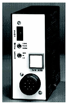
Figure 2-31. Shelf-mounted NEMA electronics unit.
Card-rack mounted electronics units contain an edge connector. The card slides into the rack cage where the male edge connector fits snuggly into the female connector in the card cage. |
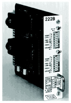
Figure 2-32. Two-channel card rack mounted electronics unit.
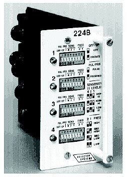
Figure 2-33. Four-channel card rack mounted electronics unit.
Two modes of operation are selectable for each electronics unit channel: presence and pulse. The presence mode of operation provides a constant output while a vehicle is over the loop detection area.
NEMA Standards require the electronics unit to sustain a presence output for a minimum of 3 minutes before tuning out the vehicle. Most units will maintain the call for periods up to 10 minutes. This mode is typically used with long loop installations on intersection approaches with the controller in the nonlocking detection memory mode.
Nonlocking detection memory is a controller function whereby the controller retains a call (vehicle detection) only as long as the presence inductive loop is occupied (vehicles are passing over or stopped on the loop). The controller drops the call if the calling vehicle leaves the detection area.
The pulse operating mode generates a short pulse (between 100 and 150 ms) each time a vehicle enters the loop detection area. Pulse operation is typically used when inductive-loop detectors are located well upstream of the intersection with the controller in the locking detection mode. That is, the controller does not drop the vehicle call when the calling vehicle leaves the detection area. Chapter 4 contains additional information about applications of locking and nonlocking controller operation.
When two loops constructed of the same wire diameter have the same loop dimensions, number of turns, and lead-in length, they have the same resonant frequency. When these two loops are near each other or when the lead-ins from these loops are in close proximity (perhaps running in the same conduit), a phenomenon known as "crosstalk" can occur. This effect is caused by an electrical coupling between the two loop channels and will often manifest itself as brief, false, or erratic actuations when no vehicles are present.
NEMA Standards require inherent, automatic, or manual techniques to be utilized to prevent crosstalk. The most common feature is a frequency selection switch that varies the operating frequency of the adjacent loop channels.
As contained in Section 15 of the NEMA standards (Appendix J), the timing features include delay and extension timing. Delay timing can be set from 0 to 30 seconds, indicating the time that the electronics unit waits, from the start of the continuous presence of a vehicle until an output begins, as shown in Figure 2-34. The output terminates when the vehicle leaves the detection area. If the vehicle leaves the detection area before the delay time has expired, no output is generated. Extension time, shown in Figure 2-35, defines the amount of time the output is extended after the vehicle leaves the detection area and can be set from 0 to 15 seconds.
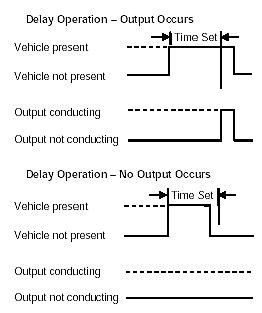
Figure 2-34. Delay operation.
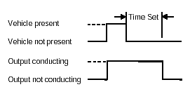
Figure 2-35. Extension operation.
Timing features can be controlled by external inputs to the electronics unit. For units with relay outputs, a delay/extension inhibit input is provided and requires 110 volts to activate. Electronics units with solid-state outputs have a delay/extension enable input, which requires a low-state DC voltage (0 to 8 volts).
A typical delayed call installation might be a semiactuated intersection with heavy right-turns-on-red from the side street, which has long loop presence detection. Using a relay output electronics unit, the side street green field output (110 volts AC) is connected to the delay/extension inhibit input. Thus, a delay is timed, allowing right-turns-on-red to be made without unnecessarily calling the controller to the side street. (Heavy right-turn movements will bring up the green anyway, as the loop will be occupied by following vehicles.) However, when the side street has the green, the delay is inhibited, permitting normal extensions of the green.
Conversely, extended call detectors could be used on high-speed approaches to an intersection operated by a basic (non-volume-density) actuated controller. Using this technique, the apparent zone of detection is extended, and different "gap" and "passage" times are created without the volume-density controls (this does not, however, replace volume-density functions). The delay/extension enable input on a solid-state output unit could be tied to the controller's "Phase On" output.(5)
Simultaneously with the evolution of the NEMA Standards, the States of California and New York developed the Type 170 controller specification.(6,7) As with the NEMA Standards, the development of this new controller was a direct response to the problems of noninterchangeability. The Type 170 system was to be interchangeable between all manufacturers supplying equipment for either state.
Unlike the NEMA Standards, which standardize functions, the Type 170 Specification standardizes hardware. The Type 170 system stipulates cabinet, controller, and all required accessories including sensors. A 170 controller is shown in Figure 2-36. The California 170 system, shown in Figure 2-37, specifies a large, base-mounted cabinet with full component layout for 28 two-channel electronics units. The New York system features a smaller, pole-mounted cabinet with 14 two-channel electronics units. New York subsequently revised its specification to require a new microprocessor. This system, denoted as a Type 179, includes the same cabinet and electronics units as the original Type 170.
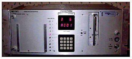
Figure 2-36. Model 170 controller (Photograph courtesy of Lawrence A. Klein).
All 170-system modules are shelf or card-rack mounted as the controllers are housed in standardized cabinets. The electronics units are mounted on an edge-connected, printed circuit board. One card slot in the cabinet will support two detector input channels. Cards supporting four detector input channels require two card slots. The electronics unit's front panel has a hand pull for insertion and removal from the input file.
An Institute of Transportation Engineers (ITE) committee composed of members from industry, Federal Highway Administration, various States and cities, and NEMA developed the concept for the advanced transportation controller (ATC). The development of a functional standard was subsequently assigned to a committee composed of affiliates from the American Association of State and Highway Transportation Officials (AASHTO), ITE, and NEMA. This group was charged with completing a consensus-based standard.(8)
The advanced transportation controller is designed to control or process data from one or more roadside devices. It operates as a general-purpose computer with a real-time operating system. One or more applications are stored in a FLASH drive. The application software is loaded and launched from the FLASH drive into dynamic random access memory (DRAM). The open architecture found in the ATC allows hardware modules and software to be purchased from a variety of vendors. A future central processor unit (CPU) option will support a daughter-board CPU that incorporates an applications program interface (API), allowing use of different microprocessors and real-time operating systems.
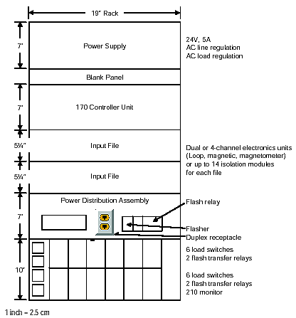
Figure 2-37. Type 170 cabinet layout (California).
The California Department of Transportation (Caltrans) has continued development of the ATC and issued standards for the development of a Model 2070 ATC.(9)
The 2070 controller contains eight module types as follows:
Figure 2-38 shows a 2070 ATC controller. An optional NEMA module may be mounted below the main chassis. Table 2-10 describes the options available for each of the modules.(9)
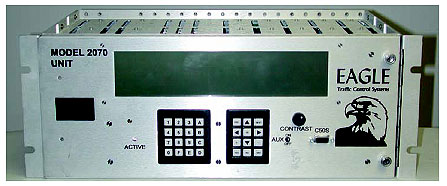
Figure 2-38. Model 2070 controller. The 2070 ATC controller is manufactured by Econolite, Eagle, Naztec, Safetran, GDI Communications, and McCain Traffic Supply at present.
Module |
Option |
Description |
|---|---|---|
CPU |
1A | Two-board CPU using Motorola 68360 microprocessor and MicroWare OS-9 operating system or PTS real-time Linux operating system. |
| 1B | One-board CPU using Motorola 68360 microprocessor and MicroWare OS-9 operating system or PTS real-time Linux operating system. | |
1C |
Daughter-board CPU using applications program interface (API) to allow use of different processors and real-time operating systems. |
|
Field I/O module |
2A | Isolates the EIA-485 internal signal line voltages between the CPU module and external equipment, and the drive and receive interfaces on external equipment. |
2B |
170 cabinet module: Field controller unit (FCU); 64-bit parallel I/O ports; other circuit functions (60-Hz square wave line synchronization signal, jumper to activate monitoring of the watchdog timer input signal (used with Model 210 cabinet monitor unit only), watchdog timer, 1-kHz reference signal, 32-bit millisecond counter, loss of communications message, logic switch to disconnect C12S connector upon command); EIA-485 serial communications; C1S, C11S, and C12S connectors; +12Vdc to +5Vdc power supply; any required software. Directly accommodates 64 inputs and 64 outputs. 2070 cabinet module: EIA-485 serial communications, DC power supply, C12S connector. Current serial bus #1 address scheme accommodates a maximum of 120 inputs and 42 outputs. |
|
Front panel assembly |
3A | FPA controller that interfaces with the CPU, 16-key pad for hexadecimal alphanumeric entry, 12-key pad for cursor control and action symbol entry, liquid crystal backlighted display of 4 lines with 40 characters per line, minimum character dimensions of 0.26-inch- (5.00-mm-)wide by 0.4- inch- (10.44-mm)-high, auxiliary switch, alarm bell. |
| 3B | FPA controller that interfaces with the CPU, 16-key pad for hexadecimal alphanumeric entry, 12-key pad for cursor control and action symbol entry, liquid crystal backlighted display of 8 lines with 40 characters per line, minimum character dimensions of 2.65 mm wide by 4.24 mm high, auxiliary switch, alarm bell. | |
3C |
No display, system serial port. |
|
Power supply |
4A | +5VDC (±5%) at 10 A, ±12VDC (±8%) at 0.5 A, +12VDC (±8%) at 1.0 A. |
4B |
+5VDC (±5%) at 3.5 A, ±12VDC (±8%) at 0.5 A, +12VDC (±8%) at 1.0 A. |
|
Chassis |
5A | Contains VME cage assembly compatible with 3U boards, metal housing, serial motherboard, backplane, power supply module supports, slot card guides, wiring harness, cover plates. |
5B |
Contains two-board CPU (option 1A) mounting assembly, metal housing, serial motherboard, backplane, power supply module supports, slot card guides, wiring harness, cover plates. |
|
Modem |
6A | Two channels of 300 to 1,200 baud asynchronous EIA-232 serial communications. |
6B |
Two channels of 0 to 9,600 baud asynchronous EIA-232 serial communications. |
|
Modem |
7A | Two channels of 300 to 1,200 baud asynchronous EIA-485 serial communications. |
7B |
Two channels of 0 to 9,600 baud asynchronous EIA-485 serial communications. |
|
NEMA interface |
8 |
Contains four NEMA connectors and EIA-485 serial communications to interface with the 2B field I/O module. Accommodates 118 inputs and 102 outputs. |
Back cover |
9 |
Protects the interface harness connecting the NEMA interface module with the 2070 controller chassis. |
Five Intelligent Transportation System (ITS) cabinet styles are manufactured to house the 2070 ATC controller and associated electronics, which includes the cabinet monitoring system, power distribution system, control and data communications systems, inductive-loop detector electronics assemblies, batteries, and power supplies. The ITS cabinets incorporate three serial buses. The first bus supports command and response communications needed for real-time control of the modules in the cabinet. A serial interface unit (SIU) can be connected to serial bus #1 to accommodate 54 inputs or outputs, including detector calls or status reports. Alternatively, each SIU can support up to 14 load switches. Serial bus #1 also sends polling commands to the emergency cabinet monitor unit (CMU) located in the power distribution assembly. The function of the CMU is to query various cabinet conditions, such as power supply voltages and line synchronization signal, and if warranted, transfer control from the ATC to a safe control mode. The second bus supports command and response communications between the 2070 controller and the controlled field devices. Serial bus #3 supports the cabinet emergency system. This system senses and monitors load outputs, various operational functions, and the bus controls and communications. When an abnormal operational condition is encountered, the cabinet emergency system controls cabinet emergency actions, through the CMU, and reports the condition to the ATC.
An advantage of serial communications between the controller and the field devices is the simplified wiring and connector utilized in the ITS cabinets as contrasted with the 104-pin C1S parallel connector found on the 170 controller or the three NEMA connectors on TS-1 controllers. The C1S connection may still be made in the 2070 using the C1S connector found on the front panel of the 2070—2 field input/output (I/O) module. Any required NEMA connections may be made through the optional NEMA module, which is mounted below the 2070.
The cabinets, constructed of aluminum sheet, contain front and rear doors. Designed to be rainproof, they are ventilated using a thermostatically controlled fan. Table 2-11 describes the cabinet styles recommended for traffic signal control and traffic management applications.
Application |
Model |
Description |
|---|---|---|
Traffic signal control1 |
340 | 4-door cabinet with P-base ground mount |
| 342 | 2-door cabinet with 170-base ground mount | |
346 |
2-door cabinet with 170-base adapter mount |
|
Traffic management1 (e.g., ramp metering) |
354 | 2-door cabinet with 170-base ground mount |
356 |
2-door cabinet with 170-base adapter mount |
1. The cabinets utilized for traffic signal control and traffic management differ in the types and numbers of cages, power supplies, power distribution and output assemblies, and serial bus harnesses.
Five models of the 2070 ATC have been designated to incorporate the VME cage and cabinet options as shown in Table 2-12.
Model number |
Description |
|---|---|
| 2070 V | 2070 containing a VME cage and mounted in a 170 or TS2 cabinet |
| 2070 N | 2070 containing a VME cage and mounted in a TS2 cabinet |
2070 L |
2070 without a VME cage and mounted in a 170 or TS2 cabinet |
2070 LC |
2070 without a VME cage and mounted in an ITS serial communications cabinet |
2070 LCN |
2070 without a VME cage and mounted in a TS2 cabinet |
Table 2-13 relates the 2070 ATC module options of Table 2-10 to the model and cabinet options of Table 2-12.
Module designator |
Module description |
Model 2070 V |
Model 2070 N |
Model 2070 L |
Model 2070 LC |
Model 2070 LCN |
|---|---|---|---|---|---|---|
— |
Unit chassis |
1 |
1 |
1 |
1 |
1 |
2070-1A |
Two-board CPU |
1 |
1 |
— |
— |
— |
2070-1B |
One-board CPU |
— |
— |
1 |
1 or |
1 or |
2070-1C |
Daughter-board CPU |
— |
— |
— |
1 |
1 |
2070-2A |
Field I/O for 170 cabinet |
1 |
— |
1 |
— |
— |
2070-2B |
Field I/O for ITS and NEMA cabinets |
— |
1 |
— |
1 or none |
1 or none |
2070-3A |
Front panel 4-line display |
1 |
1 |
— |
— |
— |
2070-3B |
Front panel 8-line display |
— |
— |
1 |
— |
— |
2070-3C |
No front panel display |
— |
— |
— |
1 |
1 |
2070-4A |
+5 VDC (±5%) at 10 A power supply |
1 |
1 |
1 or |
1 or |
1 or |
2070-4B |
+5 VDC (±5%) at 3.5 A power supply |
— |
— |
1 |
1 |
1 |
2070-5A |
VME cage assembly |
1 |
1 |
— |
— |
— |
2070-5B |
Two-board CPU mounting assembly |
1 |
1 |
— |
— |
— |
2070-8 |
NEMA interface |
— |
1 |
— |
— |
1 |
2070-9 |
2070 N back cover |
— |
1 |
— |
— |
1 |
Chapter 5 of the California Department of Transportation (Caltrans) Transportation Electrical Equipment Specifications (TEES), (reproduced in Appendix K) provides a general description, functional requirements, and electrical requirements for the Model 222 Two-Channel Loop Detector Electronics Unit and Model 224 Four-Channel Loop Detector Electronics Unit. These were illustrated in Figures 2-32 and 2-33.
Each channel in an electronics unit has panel-selectable sensitivity settings for presence and pulse operation. As with the NEMA standards, the TEES requires some mechanism to prevent crosstalk with other modules. It also requires that the selected channel not detect moving or stopped vehicles at distances of 3 ft (1 m) or more from any loop perimeter. The timing features are incorporated into the various Type 170 software programs such as the Caltrans Local Intersection Program (LIP).
Several operational characteristics influence the selection of an electronics unit model. These characteristics depend on the application and its requirements.
Tuning RangeNEMA requires that an inductive-loop detector electronics unit be capable of tuning and operating as specified over a range of inductance from 50 µH to 700 µH. For most applications, this range is adequate. Some units, however, are capable of tuning and operating over a range of 1 µH to 2,000 µH. This larger operating range permits extra long lead-in cables and/or several loops to be connected in series to one unit.
Response TimeThe time required for an electronics unit to respond to the arrival and departure of a vehicle is critical when the output is used to calculate speed and occupancy. Systems for the control of surface street traffic signals and monitoring of freeway conditions usually perform these calculations.
If the time for vehicle call pick-up is close to the time for drop-out, little or no bias in the vehicle occupancy time is introduced. If there is a significant difference, but the difference is about the same from unit to unit, a correction for the bias is easy to apply.
NEMA specifies that an electronics unit respond to the arrival or departure of a small motorcycle into and out of a 6- x 6-ft (1.8- x 1.8-m) loop within 125 ms. An automobile call must be initiated or terminated within 50 ms. NEMA also states that shorter response times might be required for specific surveillance applications that involve vehicle speeds in excess of 45 mi/h (72 km/h).
Modern traffic management systems often demand small response times. Whereas speed and occupancy measurements averaged over many vehicles to a marginal accuracy were adequate in the past, current and future applications require faster response times with greater traffic flow parameter measurement accuracies. Many of the manufacturers are responding to this need by supplying new models of electronics units with enhanced capabilities.
Recovery from Sustained OccupancyRecovery time can become critical when the electronics unit is operated in the presence mode with a long loop, say 6- x 50-ft (1.8- x 15-m), at the stop line, or four 6- x 6-ft (1.8- x 1.8-m) loops in a left-turn lane wired in a combination of series-parallel. NEMA requires that after a sustained occupancy of 5 minutes by any of the three test vehicles, the electronics unit shall recover to normal operation with at least 90 percent of the minimum specified sensitivity within 1 second after the zone of detection is vacated. If an electronics unit does not recover quickly enough, the next vehicle may not be detected at all and will be trapped until a new vehicle arrives on the loop.
During peak periods, a long loop or combination of loops may be held in detection without a break for an hour or more. In these situations, the electronics unit must continue outputting for at least an hour without dropping the detection because of an environmental tracking feature or other design defect. NEMA does not address this condition.
Sensitivity with Pavement OverlayDepth of loop wires has traditionally been considered to be a critical factor when the pavement is overlaid. However, tests conducted in Texas suggest that with high sensitivity, proper installation, and calibration, the depth at which a loop is buried should have little effect on automobile detection. In these tests, a 6- x 6-ft (1.8- x 1.8-m), five-turn loop was buried at a depth of 18.5 inch (50 cm) and encased in a 1.5-inch (1.2-cm) PVC conduit with no filler. There was no appreciable difference in the detection of large cars between the near-surface mounted loops and the deeply buried loops.
Bicycle detection was only slightly less efficient with deeply buried loops. The difference occurred at the medium sensitivity setting. The surface loop detected the bicycle 1 ft (0.3 m) outside the loop at the medium setting, while the deeply buried loop did not. The rectangular 6- x 6-ft (1.8- x 1.8-m) loop did not detect bicycles in the center portion of either the surface mounted or deeply buried loop regardless of the electronics unit sensitivity setting.
Pulse-Mode ResetThe pulse mode of operation provides an output (100 to 150 ms) that is useful in counting vehicles. An electronics unit should be capable of resetting or rephasing correctly to avoid either overcounts or undercounts when specific conditions occur. NEMA requires only that an electronics unit produce one, and only one, output pulse for a test vehicle moving at 10 mi/h (16 km/h) in the detection zone of a 6- x 6-ft (1.8- x 1.8-m) loop.
When vehicles are counted simultaneously in two or more lanes, a separate electronics unit and loop are recommended for each lane to guarantee accuracy. This approach can be implemented for a small additional cost over the use of a single electronics unit and a wide loop.
Although NEMA does not address this point, some electronics units provide failsafe operation with faulty loops, i.e., grounded or open loops. The use of a loop isolation transformer permits these models to operate if the loop insulation is leaky or even shorted completely to ground at a single location.
Isolation allows "balanced to ground" operation of the loop circuit. This reduces the effect of the loop and lead distributed capacitance and, hence, thermal- and moisture-induced changes in the capacitance. The balanced operation also minimizes loop circuit coupling from lead-in cables in common conduits. If the loop breaks, this design fails in a "safe" way by holding a constant call, thus keeping traffic moving and avoiding trapping any vehicles. Such operation is, however, very inefficient.
An extensive study into the effects of lightning related electrical surge problems was conducted by the Ontario Ministry of Transportation.(10) The major conclusions of the study were:
NEMA requires that electronics units withstand the same power-line transients specified for controller units. The input terminals to the electronics unit must be able to withstand 3,000 volts. The primary to secondary insulation of the input (loop-side) transformer protects against "common mode" lightning voltages.
With one electronics unit model, differential lighting protection consists of a four-element protective circuit composed of the input resistors, a neon tube, transformer leakage inductance, and the diode path across the secondary. Differential lightning-induced currents are also potentially damaging. These currents are shunted through neon bulbs, limiting the voltage across the transformer.
Specifications for Model 170 controller cabinets require that lightning protection be installed within the inductive-loop detector electronics unit. The protection allows the electronics unit to withstand the discharge of a 10-microfarad capacitor charged to ±1,000 volts directly across the electronics unit input pins with no loop load present. The protection must also withstand the discharge of a 10-microfarad capacitor charged to ±2,000 volts directly across either the electronics unit input inductance pins or from either pin to earth ground. The electronics unit chassis is grounded and a dummy resistive load of 5 ohms is attached to the pins.
The Model 170 specifications also include provisions for preventing interference between channels in a given electronics unit as well as between units. The prevention techniques may be either manual or automatic.
Two types of magnetic field sensors are used for traffic flow parameter measurement, the two-axis fluxgate magnetometer (that detects stopped and moving vehicles) and the magnetic detector, more properly referred to as an induction or search coil magnetometer (that typically detects only moving vehicles). Magnetic sensors were introduced in the l960s as an alternative to the inductive-loop detector for specific applications. A magnetic sensor is designed to detect the presence or passage of a vehicle by measuring the perturbation in the Earth's quiescent magnetic field caused by a ferrous metal object (e.g., a vehicle) when it enters the detection zone of the sensor. An example of a magnetic sensor installation is shown in Figure 2-39.
Figure 2-39. Magnetic sensor installation.
Early magnetic sensors were utilized to determine if a vehicle had arrived at a "point" or small-area location. They actuated controller phases that operated in the locking detection memory mode. They were also effective in counting vehicles. Modern two-axis fluxgate magnetometers are used for vehicle presence detection and counting. Unlike the inductive-loop detector, the magnetometer will usually operate on bridge decks where uncoated steel is present and cutting the deck pavement for loop installation is not permitted. The magnetometer probe and its lead-in wire tend to survive in crumbly pavements longer than ordinary loops. Another benefit is that they require fewer linear feet of sawcut.
Magnetic sensor operation is based on detecting the concentration of the Earth's magnetic flux above and below a ferrous metal vehicle. |
Magnetic sensor operation is based on an Earth magnetic field model that depicts the Earth as a large bar magnet with lines of flux running from pole to pole as illustrated in Figure 2-40. A vertical axis magnetometer requires the vertical component of the Earth's magnetic field to exceed 0.2 Oersteds. Therefore, magnetometers that contain only vertical axis sensors cannot be used near the Equator, where the magnetic field lines are horizontal. This situation is illustrated in Figure 2-41 by the cross-hatched area near the equator, which defines the region that is not suitable for vertical axis magnetometers. However, modern fluxgate magnetometers are built with both horizontal and vertical axis sensors. Therefore, they can operate anywhere on the face of the Earth.
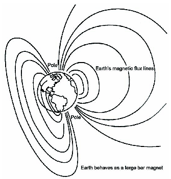
Figure 2-40. Earth's magnetic flux lines.
Modern fluxgate magnetometers built with both horizontal and vertical axis sensors can operate in the equatorial belt region shown in Figure 2-41. |
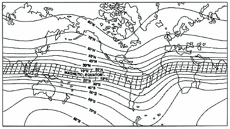
Figure 2-41. Equatorial belt showing where Earth's magnetic field is too small for deployment of simple vertical axis magnetometers between 20 degrees north and 20 degrees south of the Equator.
An iron or steel vehicle distorts the magnetic flux lines because ferrous materials are more permeable to magnetic flux than air. That is, the flux lines prefer to pass through the ferrous vehicle. As the vehicle moves along, it is always accompanied by a concentration of flux lines known as its "magnetic shadow" as illustrated in Figure 2-42. There is reduced flux to the sides of the vehicle and increased flux above and below it. A magnetometer installed within the pavement detects the increased flux below the vehicle.
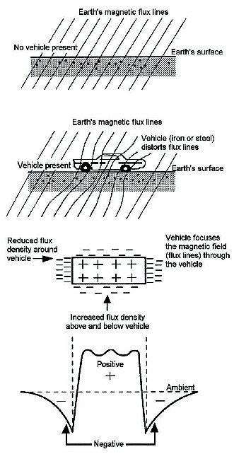
Figure 2-42. Distortion of Earth's quiescent magnetic field by a ferrous metal vehicle.
Two-axis fluxgate magnetometers contain sensors that detect both the vertical and horizontal components of the Earth's magnetic field and any disturbances to them. One of the secondary windings in a two-axis fluxgate magnetometer senses the vertical component of the vehicle signature, while the other, offset by 90 degrees, senses the horizontal component of the signature. The horizontal axis of the magnetometer is usually aligned with the traffic flow direction to provide in-lane presence detection and adjacent lane vehicle rejection. Fluxgate magnetometers measure the passage of a vehicle when operated in the pulse output mode. In the presence mode, they give a continuous output as long as either the horizontal or vertical signature exceeds a detection threshold.
The data provided by fluxgate magnetometers are the same as from inductive loops. Typical applications are vehicle presence detection on bridge decks and viaducts where inductive loops are disrupted by the steel support structure or weaken the existing structure, temporary installations in freeway and surface street construction zones, and signal control.
The infusion of modern digital processing and radio frequency (RF) communications technology in the area of magnetic anomaly detection have generated new designs, such as the self-powered vehicle detector (SPVD) and Groundhog magnetometers, justifying a reassessment of their supplementary role in vehicle detection. In addition, an array of magnetometers sharing a common signal processor has the potential to locate, track, and classify vehicles in a multilane scenario using a row of above-ground sensors.(11)
Figure 2-43 shows the electrical configuration of the core and primary and secondary windings typically found in a magnetometer sensor. The core and windings create a small, stable transformer-like element. The two primary and two secondary windings are placed over a single strip of Permalloy core material, which is treated to produce special satur4able magnetic properties.
Figure 2-43. Magnetometer sensor electrical circuit (notional).
Sensor operation is based on generating a second harmonic signal from the open saturable core, which is oriented to provide maximum sensitivity to disturbances in the Earth's magnetic field. A triangular wave excitation current of suitable frequency (typically 5 kHz) is applied to the two primary windings connected in series opposition. The secondary windings, which also carry the DC bias to neutralize the quiescent Earth field, are connected in series, enhancing the supply of second-harmonic signal to the sensor's electronics unit.
A polyurethane casing is often used for abrasion resistance. It also makes the probe impervious to moisture and chemically resistant to all normal motor vehicle petroleum products. If the pavement is soft, some probes may tilt, causing them to change their orientation and lose sensitivity. A length of PVC pipe can be used to hold these probes vertical.
Figure 2-44 contains an electrical circuit diagram of a magnetometer sensor and companion electronics unit that performs signal amplification. Provided the ambient magnetic field is stable and exceeds about 16 ampere per meter (20,000 gamma), the magnetic shadow cast by a vehicle causes a local field increase of the order of 20 percent. The switch-like action of the magnetic material in the sensor induces a signal change several times this amount. This detection principle provides high sensitivity and signal-to-noise ratio.
Figure 2-44. Magnetometer sensor probe and electronics unit equivalent electrical circuit.
Since magnetometers are passive devices, they do not transmit an energy field. Therefore, a portion of the vehicle must pass over the sensor for it to be detected. Consequently, a magnetometer can detect two vehicles separated by a distance of 1 foot (0.3 m). This potentially makes the magnetometer as accurate as or better than the inductive-loop detector at counting vehicles.
Conversely, the magnetometer is not a good locator of the perimeter of the vehicle, with. There is an uncertainty of about ±1.5 ft (45 cm). A single magnetometer is, therefore, seldom used for determining occupancy and speed in a traffic management application. Two closely spaced sensors are preferred for that function.
Magnetometers are sensitive enough to detect bicycles passing across a 4-ft (1.2-m) span when the electronics unit is connected to two sensor probes buried 6 inches (16 cm) deep and spaced 3 ft (0.9 m) apart. Magnetometers can hold the presence of a vehicle for a considerable length of time and do not exhibit crosstalk interference. Vehicle motion is not required for detection by two-axis fluxgate magnetometers.
One channel of an electronics unit can support as many as 12 series-connected sensors. However, the sensitivity is divided among the probes so that there is a loss in sensitivity per probe when more than one is used per channel. The electronics unit will detect with a vehicle over one out of five probes in the series (i.e., 20 percent sensitivity on each probe).
Specific magnetometer electronics units are matched with various sensor probes. Some units provide only signal amplification and relay or solid state-state outputs that indicate the passage or presence of a vehicle, while others add additional features such as background compensation and sensitivity selection. Some include 2 or more independent detection channels, which can accept 1 to 12 series-connected sensors on each channel.
Calibration procedures are utilized to compensate the electronics unit for the magnetic environment around the roadway sensors. A check is made prior to tuning to assure that no vehicles or movable ferrous equipment are within 20 ft (6 m) of a sensor. Some magnetometer electronics units include, for each channel, a calibration knob that is turned until a pilot light flashes, indicating that the ambient magnetic field has been neutralized. Some magnetometer sensors do not offer a delayed-call timing feature.
Four operating modes are typically available. These are selected on the front panel of the electronics unit and include:
Chapter 6 of the Caltrans Type 170 Specification contains specifications for the Model 227 magnetometer sensing element and the Model 228 two-channel electronics unit. The electronics unit is defined only for a two-channel version. Each channel operates one to six Model 227 sensors. The electronics unit produces an output signal whenever a vehicle passes over one or more of the sensors.
Since a magnetometer measures the passage or presence of a vehicle, two modes of operation are provided by the electronics unit: pulse, which gives an output closure of 125 ± 25 ms for each vehicle entering the zone of detection, and presence, which gives a continuous output as long as a vehicle occupies the detection zone.
Figure 2-45 shows the self-powered vehicle detector. Applications include permanent and temporary installations on freeways and surface streets or where mounting under bridges or viaducts is desired. The SPVD-2 approximates the shape of a 5-inch (13-cm) cube and fits into a cylindrical hole of 6-inch (15-cm) diameter and about 7-inch (18-cm) depth. The upper 2 inches (5 cm) of the hole is filled with cold patch or other sealant that can be removed when the battery needs replacing.
This two-axis fluxgate magnetometer has a self-contained battery and transmitter that broadcasts passage or presence information at 47 MHz over a 400- to 600-ft (122- to 183-m) range to a receiver that can be located remotely in a controller cabinet. The transmitting frequency can be selected to operate in a quiet frequency band, i.e., one where other licensed and unlicensed devices are not operating in the local region. A direct connection (lead-in cable) is not required—a transmitting antenna is built into the housing that encloses the magnetometer electronics and battery. When operated in the presence mode, presence is maintained with a voltage latching circuit for as long as the vehicle is in the detection zone. The sensitivity can be adjusted to restrict vehicle detection to the lane in which the device is installed.
Figure 2-45. SPVD-2 magnetometer system (Photograph courtesy of Midian Electronics, Tucson, AZ).
The SPVD is microprocessor controlled and self-calibrating, i.e., it can be installed and adapt to a location in either the Northern or Southern Hemisphere. The battery life is a function of traffic volume and battery type. With an average of 10,000 arrivals and 10,000 departures per day, the alkaline battery is quoted by the SPVD manufacturer as lasting approximately 4 years. Turning off the departure pulse adds another year or two of battery life. A low battery warning is transmitted to the receiver to indicate that 5 to 6 months of battery life remain.
Figure 2-46 illustrates the Groundhog magnetometer sensors. The G-1 fits into a hole of 4.5-inch diameter and 7.5-inch depth (115-mm diameter x 190-mm depth). The G-2 models require a 6.75-inch diameter hole with 7.5-inch depth (172-mm diameter x 190-mm depth). A shorter G-3 model series was designed for installation under a bridge deck. These models had the same functionality as the G-1 and G-2 models. The G-4 series sensors are designed to fit into the G-3 housing, which requires a 6-inch diameter hole of 3.25-inch depth (152.4-mm diameter x 82.6-mm depth).
Buried in the roadway, the G-1 and G-2 sensors transmit their data over the 908 to 922 MHz spread spectrum band to a local base unit located within 200 m (656 ft) of the sensor. The G-4 series sensors transmit data using the 2.45 GHz spread spectrum band. The base unit can be powered from batteries recharged by solar energy.
Groundhog magnetometers incorporate a bridge circuit that is balanced to output zero voltage in the absence of a vehicle and a nonzero voltage when a vehicle enters the detection zone. The G-1 model provides volume, lane occupancy, and road surface temperature. The G-2 adds vehicle speed reported in up to 15 bins, vehicle class in terms of vehicle length reported in up to 6 bins, and a wet/dry pavement indicator. In addition to the previously mentioned traffic parameters, the G-2wx provides chemical analysis for measuring the quantity of anti-icing chemicals on the road surface. The G-4C provides vehicle count only, while the G-4CS provides vehicle count, speed, and classification. The G-4WX adds environmental monitoring of road surface temperature from —67 °Fahrenheit (F) to 185 °F (—55 ° Celsius (°C) to 85 °C) and road surface wet or dry condition to the G-4CS data set.
Figure 2-46. Groundhog magnetometer sensors
(Photographs courtesy of Nu-Metrics, Uniontown, PA).
The G-1 sensor is powered from 2 lithium batteries with a quoted battery life of 5 years based on 18,000 cars/day and report intervals of 2 minutes. The G-2 requires 4 lithium batteries with a quoted battery life of 5 years based on 18,000 cars/day and report intervals of 1 minute. The G-4 also operates from 4 lithium batteries for up to 5 years, depending on annual average daily traffic (AADT) and polling interval.
The magnetic detector is a simple, inexpensive and rugged device that is capable of only a pulse output. It can be used for traffic-actuated signal control or to simply count vehicles. Some magnetic sensors are installed inside a nonferrous conduit by boring under the roadway. Others are mounted under bridges or in holes cored into the road surface.
Magnetic detectors, i.e., those based on induction or search coil magnetometers, also respond to perturbations in the Earth's magnetic field produced by vehicles passing through the detection zone. The axis of the coil in all magnetic detectors is installed perpendicular to the traffic flow and has an associated spherical detection zone. The distortion and change of the magnetic flux lines with respect to time induces a small voltage that is amplified in an electronics unit located in the controller cabinet. This signal is interpreted by the controller as the passage of a vehicle and produces a call if appropriate.
Magnetic detectors contain a highly permeable magnetic core on which several coils are wound, each with a large number of turns of fine wire, and connected in series. Disturbed lines of magnetic flux cut the turns of the coil and create an output for as long as the vehicle is in motion through the detection zone. Minimum speeds of 3 to 10 mi/h (5 to 16 km/h) are required to produce an actuation. A single magnetic detector does not detect stopped vehicles; therefore, it cannot be used as a presence detector. However, multiple units of some devices can be installed and used with specialized signal processing to generate vehicle presence.
Magnetic detectors respond to flux changes in the lane under which they are buried and to flux changes in adjacent lanes. However, the signal processing is designed to ignore the lower magnitude signals generated in adjacent lanes and analyze only the larger signals produced by vehicles in the lane containing the sensor.
These detectors provide volume, occupancy, and speed data based on the detection zone size and an assumed vehicle length. The historical criteria for their selection are traffic volume accuracy, sensitivity, output data rate, no requirement to detect stopped vehicles, and cost. Magnetic detectors are well suited for snow-belt States where deteriorated pavement and frost break wire loops and where subsurface sensors are desired but the pavement cannot be cut.(2) They also perform well in hot climates where asphalt pavements can become soft from the sun heat load.
Magnetic detector models differ in their installation and size. Summary specifications of several models are given below.
Specifications for the Model 231 sensing element and Model 232 two-channel electronics unit are found in Chapter 5 of the Caltrans TEES document (see Appendix K).
Each individual sensor channel and its associated magnetic sensing element operate independently and produce an output signal when a vehicle passes over the embedded sensing element. The solid-state electronics unit, located in the controller cabinet, activates the controller by amplifying the voltage induced in the sensing element by a passing vehicle.
The Model 231 sensor, shown in Figure 2-47, is installed by tunneling under the roadway 14 to 24 inches (356 to 610 mm) and inserting the sensor into a nonferrous plastic or aluminum conduit. In bridge or overpass installation, the sensor is fastened to the understructure directly below the center of the traffic lane. The sensor has a diameter of 2.25 inches (57 mm) and a length of 21 inches (533 mm). The speed data, available from the electronics modules, are based on a detection zone length of 6 ft (1.8 m) and an assumed vehicle length of 18 ft (5.5 m).
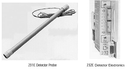
Figure 2-47. Magnetic probe detector
(Photographs courtesy of Safetran Traffic Systems, Colorado Springs, CO).
Another type of passive magnetic detector is flush-mounted with the surface of the roadway. It is approximately 3 x 5 x 20 inches long (76 x 127 x 508 mm) encased in a cast aluminum housing.
Figure 2-48 depicts other forms of magnetic detectors called microloop probes. The Model 701 probe is inserted into 1-inch (25-mm) diameter holes bored to a depth of 16 to 24 inches (406 to 610 mm). The Model 702 probe is inserted into 3-inch (76-mm) Schedule 80 PVC placed 18 to 24 inches (457 to 610 mm) below the road surface using horizontal drilling from the side of the road. Often two or more microloop probes are connected in series or with conventional wire loops to detect a range of vehicle sizes and obtain required lane coverage. The Model 702 microloop probe can be connected in rows of three to generate signals that detect stopped vehicles. Application-specific software from 3M is also needed to enable stopped vehicle detection.
Model 701 Model 702
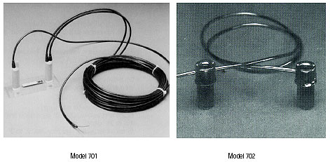
Figure 2-48. Microloop probes (Photographs courtesy of 3M Company, St. Paul, MN).
The use of video and image processing technology as a substitute for inductive-loop detectors was first investigated during the mid-1970s. This research was funded by the U.S. Federal Highway Administration (FHWA) and performed by the Jet Propulsion Laboratory. The project combined television camera and video processing technology to identify and track vehicles traveling within the camera's field of view.(12) During the 1970s and 1980s, parallel efforts were undertaken in Japan, the United Kingdom, Germany, Sweden, and France. These investigations addressed the problems and limitations of existing roadway sensors in attempting to fulfill requirements for state-of-the-art control of traffic and detection of incidents.
As a follow-on to the initial FHWA project, a video image processor was developed by University of Minnesota research personnel.(13) Dubbed the Video Detection System (VIDS), it was jointly funded by FHWA, Minnesota Department of Transportation, and the University of Minnesota. The sensor provided volume and occupancy data equivalent to those from multiple inductive-loop detectors. Full bandwidth imagery and the traffic data were transmitted to a central location for interpretation and management of traffic.
Three classes of VIP systems are now produced or in development: tripline, closed-loop tracking, and data association tracking. Tripline systems, as used by the sensors in Figures 2-49a, 2-49b, 2-49c, and 2-49d, operate by allowing the user to define a limited number of linear detection zones on the roadway in the field-of-view of the video camera. When a vehicle crosses one of these zones, it is identified by noting changes in the properties of the affected pixels relative to their state in the absence of a vehicle. Tripline systems that estimate vehicle speed measure the time it takes an identified vehicle to traverse a detection zone of known length. The speed is found as the length divided by the travel time.
Surface-based and grid-based analyses are utilized to detect vehicles in tripline VIPs. The surface-based approach identifies edge features, while the grid based classifies squares on a fixed grid as containing moving vehicles, stopped vehicles, or no vehicles.
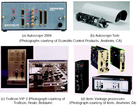
Figure 2-49. Tripline video image processors.
The advent of VIP tracking sensors has been facilitated by low-cost, high-throughput microprocessors. Closed-loop tracking systems, as used in some VIPs, as illustrated in Figure 2-50, detect and continuously track vehicles along larger roadway sections. The tracking distance is limited by the field of view, mounting height, and resolution of the camera. Multiple detections of the vehicle along the track are used to validate the detection and improve speed estimates. Once validated, the vehicle is counted and its speed is updated by the tracking algorithm.(14) These tracking systems may provide additional traffic flow data such as lane-to-lane vehicle movements. Thus, they have the potential to transmit information to roadside displays and radios to alert drivers to erratic behavior that can lead to an incident. Their ability to monitor turning movements on arterials may allow more frequent updating of signal timing plans.
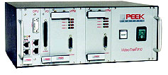
Figure 2-50. Closed-loop tracking video image processor.
Data association tracking systems identify and track a particular vehicle or groups of vehicles as they pass through the field of view of the camera. The computer identifies vehicles by searching for unique connected areas of pixels. These areas are then tracked from frame-to-frame to produce tracking data for the selected vehicle or vehicle groups.(15-17) Objects are identified by markers that are derived from gradients and morphology. Gradient markers utilize edges, while morphological markers utilize combinations of features and sizes that are recognized as belonging to known vehicles or groups of vehicles.(18) Data association tracking can potentially provide link travel time and origin-destination pair information by identifying and tracking vehicles as they pass from one camera's field of view to the next camera's field of view.
Modern video image processors conserve transmission bandwidth by performing signal processing in microprocessors located either in the camera (as for example in the Autoscope Solo) or in modules mounted in a controller cabinet at the roadside as shown on the upper shelf in Figure 2-51. The data are used locally by the controller for signal timing and to characterize the level of service on freeways, for example. The data can also be transmitted to the traffic operations center over low-bandwidth communications media for incident detection and management, database update, and traveler information services.
By multiplexing video images from several cameras on one transmission line and sending the video only when requested, operating costs associated with leased transmission media are further reduced. By extending the identification of vehicles or groups of vehicles from the field of view of one camera into that of another, vehicles can be tracked over greater distances to compute link travel times and generate origin-destination pair data. The output products from the traffic management center can be forwarded to other transportation management centers, emergency service providers, and information service providers.
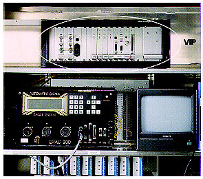
Figure 2-51. Video image processor installed in a roadside cabinet
(Photograph courtesy of Iteris, Anaheim, CA).
Image formatting and data extraction are performed with firmware that allows the algorithms to run in real time. The hardware that digitizes the video imagery is commonly implemented on a single formatter card in a personal computer architecture or in microprocessors located in the camera housing. Once the data are digitized and stored by the formatter, spatial and temporal features are extracted using a series of image processing algorithms to differentiate vehicles from roadway or background pixels.
In the concept illustrated in Figure 2-52, a camera is used to acquire imagery of the traffic flow. The images are digitized and stored in memory. A detection process establishes one or more thresholds that limit and segregate the digitized data passed on to the rest of the image processing algorithms. It is undesirable to severely limit the number of potential vehicles during detection, for once data are removed they cannot be recovered. Therefore, false vehicle detections are permitted at this stage since the declaration of actual vehicles is not made at the conclusion of the detection process. Rather algorithms that are part of the classification, identification, and tracking processes still to come are relied on to eliminate false vehicles and retain the real ones.(19) Image segmentation is used to divide the image area into smaller regions (often composed of individual vehicles) where features can be better recognized. The feature extraction process examines the pixels in the regions for preidentified characteristics that are indicative of vehicles. When a sufficient number of these characteristics are present and recognized by the processing, a vehicle is declared present and its flow parameters are calculated.
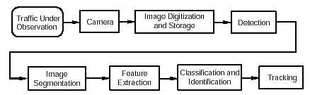
Figure 2-52. Conceptual image processing for vehicle detection, classification, and tracking.
(Source: L.A. Klein, Sensor Technologies and Data Requirements for ITS (Artech House, Norwood, MA, 2001)).
Artificial neural networks are another form of processing used to classify and identify vehicles, measure their traffic flow parameters, and detect incidents.(20) Features are not explicitly identified and sought when this processing approach is used. Rather an electrical network that emulates the processing that occurs in the human brain is trained to recognize vehicles. The digital imagery is presented to the trained network for vehicle classification and identification.
VIPs with tracking capability use Kalman filtering techniques to update vehicle position and velocity estimates.(21) The time trace of the position estimates yields a vehicle trajectory. By processing the trajectory data, local traffic parameters (e.g., flow and lane change frequency) can be computed. These parameters, together with vehicle signature information (e.g., time stamp, vehicle type, color, shape, position, and speed), can be communicated to the traffic management center.(22) Tracking vehicle subfeatures. such as edges, corners, and two-dimensional patterns, rather than entire vehicles, has been proposed to make the VIP robust to partial occlusion of vehicles in congested traffic. Preliminary results with this technique show insensitivity to shadows since shadow subfeatures tend to be unstable over time, especially in congestion. Camera mounting position and continued full occlusion of smaller vehicles by trucks still deteriorate performance.(23,24)
A signal processing technique implemented by Computer Recognition Systems (Wokingham, Berkshire, England; Knoxville, TN) incorporates wireframe models composed of line segments to represent vehicles in the image. This approach claims to provide more unique and discriminating features than other computationally viable techniques.
The artificial neural network approach is incorporated by Nestor Traffic Systems, Inc. (Providence, RI) in their VIP products. An advantage of the Nestor implementation is that the camera can be repositioned for data acquisition and surveillance.(25) VIPs that utilize tracking offer the ability to warn of impending incidents due to abrupt lane changes or weaving, calculate link travel times, and determine origin-destination pairs. The tracking concept is found in the VideoTrak 905 and 910 by Peek Traffic-Transyt, the Traffic Analysis System by Computer Recognition Systems, MEDIA4 developed by Citilog (Paris, France), and the IDET-2000 by Sumitomo (Japan).
VIP signal processing is continually improving its ability to recognize artifacts produced by shadows, illumination changes, reflections, inclement weather, and camera motion from wind or vehicle-induced vibration. However, artifacts persist and the user should evaluate VIP performance under the above conditions and other local conditions that may exist. In their 1998 report to the TRB Freeway Operations Committee, the New York State Department of Transportation (NYSDOT) stated that one VIP model had difficulty detecting vehicles on a roadway lightly covered with snow in good visibility. Another model did not experience this problem. A 2004 evaluation of VIP performance by Purdue University described significant false and missed vehicle detections as compared with loops, even when the cameras were installed at vendor-recommended locations at a well-lighted intersection.(24)
Figure 2-53 illustrates the effect day-to-night illumination change has on VIP performance. The VIP cameras viewed downstream traffic from a mast arm position approximately 25 ft (7.6 m) above the curb and middle lanes of a three-lane roadway. Shortly after 1,900 hours, there are changes in the slopes of the VIP vehicle count data due to either degradation in performance of the daytime algorithm or the different performance of the nighttime algorithm.(11)
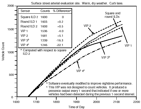
Figure 2-53. Vehicle count comparison from four VIPs and inductive-loop detectors
(source: L.A. Klein and M.R. Kelley, Detection Technology for IVHS: Final Report, Report No. FHWA-RD-95-100 (USDOT, FHWA, Washington, D.C.,1995)).
Figure 2-54 shows the effects of day-night illumination changes from another VIP test.(26) The camera faced upstream traffic, mounted approximately 25 ft (7.6 m) above the road surface. The camera was placed on a mast arm extension on the left side of a roadway, which contained three through lanes and a dedicated right-turn lane. The VIP tracked vehicles and provided flow rate, lane speed, queue length, density, number of left and right turning vehicles, and approach stops. VIP performance was not optimized because of a number of factors: low camera sensitivity that was more problematical at low light levels, focal length of lens not matched to the viewing distance, low camera resolution, low and offcenter camera mounting height, inadequate video signal output from camera to drive both the VIP and video cassette recorder, no sun shade, and camera vibration with winds greater than 10 mi/h (16 km/h).
Because of these nonideal conditions, a quantitative comparison of the VIP-generated traffic flow parameters with ground truth is not given here. Instead, the focus is on the effect that illumination changes have on VIP performance, albeit exaggerated by many of the conditions cited above. The effects of low camera sensitivity and inadequate video signal are most apparent at dawn, night, and dusk where the false alarm and missed vehicle errors (0.15, 0.44, and 0.91, respectively) are largest. These results demonstrate the importance of proper camera and lens selection, camera mounting, and illumination in maximizing VIP performance.
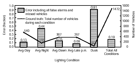
Figure 2-54. VIP vehicle count errors under varying illumination conditions. Low camera sensitivity, improper focal length of lens, low camera resolution, nonideal camera mounting height, inadequate video signal, and lack of sun shade contributed to degraded performance
(source: Traffic Surveillance and Detection Technology Development: Phase II and III Test Results, Troy, MI, JPL Pub. D-15779 (California Institute of Technology, Jet Propulsion Laboratory, Pasadena, CA, May 1998)).
Heavy congestion that degraded early VIPs does not appear to present as great a problem to more modern systems. Combined results for clear and inclement weather show vehicle volume, speed, and occupancy measurement accuracies in excess of 95 percent using a single detection zone and a camera mounted at a sufficiently high height. VIPs with single or multiple detection zones per lane can be used to monitor traffic on a freeway. For signalized intersection control, where vehicle detection accuracies of 100 percent are desired, the number of detection zones per lane is increased to between two and four, depending on the camera mounting and road geometry. However, even with multiple detection zones, vehicle detection accuracy can degrade to 85 percent or less with side-viewing cameras that are not mounted high enough (on the order of 30 ft (9 m) rather than 50 ft (15 m)) or are not directly adjacent to the roadway.(27-29) The study that produced these results also reported that vehicle detection was sometimes sensitive to vehicle-to-road color contrast.
Additional merits and issues associated with application of video image detection at signalized intersections are reported in a 2004 survey conducted by the Urban Transportation Monitor.(30) The survey contained responses from 120 jurisdictions. The survey results were summarized by the Monitor as follows:
...the use of video detection at signalized intersections is clearly controversial with many respondents having very strong opinions (both positive and negative) about its application. For example, 35% of the respondents experienced more complaints with the application of video detection, 19% indicated they experienced fewer complaints, and the balance indicated that the number of complaints have remained the same. On the other hand, 66% of respondents indicated that they will increase their application of video detection while 12% indicated that they will actually decrease their applications.
These differences in experience and attitude are also reflected in the answers to the questions related to the main advantages and disadvantages compared to inductive loops. About the same number of positive replies (advantages) and negative replies (disadvantages) were received. Most frequent positive replies had to do with the ability of video detection to cope with changes in the detection zones due to restriping and the most frequent negative replies had to do with the inability of video detection to provide adequate results (or any results at all) during inclement weather (fog, heavy snow) and when the sun shines directly at the video camera.
What seems to be clear is that agencies who are contemplating the use of video detection should approach it carefully as there are many pitfalls, as indicated in the survey results. It seems clear that it is also important to make sure a vendor is selected that can provide the latest improvements in video detection technology.
Video image processor cameras can be deployed to view upstream or downstream traffic. The primary advantage of upstream viewing is that incidents are not blocked by the resultant traffic queues as described in Table 2-14. However, tall vehicles such as trucks may block the line of sight, and headlights may cause blooming of the imagery at night. With upstream viewing, headlight beams can be detected as vehicles in adjacent lanes on curved road sections. Downstream viewing conceals cameras mounted on overpasses so that driver behavior is not altered. Downstream viewing also makes vehicle identification easier at night through the information available in the taillights and enhances track initiation because vehicles are first detected when close to the camera.(31)
Upstream viewing |
Downstream viewing |
|---|---|
|
|
Although some manufacturers quote a maximum surveillance range for a VIP of ten times the camera mounting height, conservative design procedures limit the range to smaller distances because of factors such as road configuration (e.g., elevation changes, curvature, and overhead or underpass structures), congestion level, vehicle mix, and inclement weather. The impact of reduced headway on the effective surveillance range is calculated from the distance d (along the roadway from the base of the camera mounting structure to the vehicles in question) at which the VIP can distinguish between two closely spaced vehicles. The distance d depends explicitly on camera mounting height, vehicle separation or gap, and vehicle height, as illustrated in Figure 2-55.
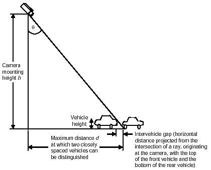
Figure 2-55. Distinguishing between two closely spaced vehicles
(source: L.A. Klein, Sensor Technologies and Data Requirements for ITS (Artech House, Norwood, MA, 2001)).
If the roadway does not have a grade, d is approximated by
 (2-63)
where:
h = camera mounting height
Vehgap = intervehicle gap
Vehheight = vehicle height.
Distance d is also implicitly dependent on the pixel size or instantaneous field-of-view of the camera, as larger values of d may not be realized without a correspondingly small pixel size. Figure 2-56 contains plots of distance d versus vehicle separation based on Equation 2-63 for vehicle heights of 5 ft (1.5 m), representative of a passenger automobile, and 13 ft (4 m), representative of a larger commercial vehicle.
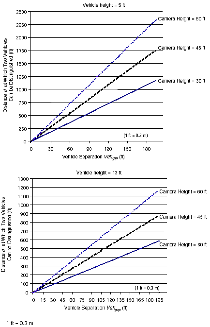
Figure 2-56. Distance d along the roadway at which a VIP can distinguish vehicles: (top) vehicle height = 5 ft (1.5 m), (bottom) vehicle height = 13 ft (3.9 m). These values may be further limited by road configuration, congestion level, vehicle mix, inclement weather, and pixel size.
Other factors that affect camera installation include vertical and lateral viewing angles, number of lanes observed, stability with respect to wind and vibration, and image quality. VIP cameras can be mounted on the side of a roadway if the mounting height is high, i.e., 50 ft (15.2 m) or higher. For lower mounting heights of 25 to 30 ft (7.6 to 9.1 m), a centralized location over the middle of the roadway area of interest is required. However, the lower the camera mounting, the greater is the error in vehicle speed measurement—the measurement error is proportional to the vehicle height divided by the camera mounting height. False detection and missed detections also increase at lower camera mounting heights. (See references 14, 24, and 32-34.)
The number of lanes of imagery analyzed by the VIP is of importance to ensure that the required observation and analysis region is supported by the VIP. For example, if the VIP provides data from detection areas in three lanes, but five must be observed, that particular VIP may not be appropriate for the application.
VIPs that are sensitive to large camera motion may be adversely affected by high winds since the processor may assume that the wind-produced changes in background pixels correspond to vehicle motion. Software that automatically learns the new operating environment and road configuration on which a VIP is operating has entered the market place. One such tool developed by Citilog advertises that no configuration, calibration, or parameter entry are necessary for their software to operate with existing pan, tilt, and zoom cameras for detection of stopped vehicles, congestion, and accidents.
Image quality and interpretation can be affected by cameras that have automatic iris and automatic gain control. An automatic iris adjusts the light level entering the camera not only when roadway background lighting changes, but also when headlights, reflections from windshields and bumpers, or white or bright objects are in the field of view. Automatic gain control momentarily reduces the sensitivity of the camera to the same phenomena. These controls impair the ability of cameras with a low signal-to-noise ratio to detect following vehicles when they restrict entering light levels.(26) When the camera responds by quickly darkening the entire picture and then recovering, some systems interpret this as an extra vehicle.
In tests conducted by California Polytechnic University at San Luis Obispo (Cal Poly SLO), automatic iris and gain controls were disabled in an effort not to handicap the detection ability of the VIPs they evaluated.(35) In followup tests several years later, Cal Poly SLO found VIPs better able to compensate for light level changes when the automatic iris responded slowly to variations in light entering the camera.(36) This finding was confirmed by the Texas Transportation Institute (TTI), which specifies its VIP cameras to have damped iris and automatic gain controls.(32)
When a traffic management agency wishes to use a single camera to provide imagery to a VIP and to obtain video surveillance with pan, tilt, and zoom controls, it is necessary to reposition the camera to its calibrated position for each VIP application. If the camera is not in the calibrated position, the performance of the VIP is degraded. If remote control of cameras and their return to calibrated fields of view is not feasible, then separate cameras may be required to perform automated traffic data collection and video surveillance. Some VIPs can automatically recalibrate the field of view for a new camera position using specialized algorithms.
Even without its association with VIPs, closed-circuit television (CCTV) has become a valuable asset for traffic management. In addition to its primary task of incident verification on freeways, CCTV is used for other applications in freeway and corridor traffic management. These include:
Current CCTV technology allows viewing of 0.25 to 0.5 mi (0.4 to 0.8 km) in each direction if the camera mounting, topography, road configuration, and weather are ideal. The location for CCTV cameras is dependent on the terrain, number of horizontal and vertical curves, desire to monitor weaving areas, identification of high-incident locations, and the need to view ramps and arterial streets. Each prospective site must be investigated to establish the camera range and field of view that will be obtained as a function of mounting height and lens selection.
Two types of microwave radar sensors are used in roadside applications, those that transmit continuous wave (CW) Doppler waveforms and those that transmit frequency modulated continuous waves (FMCW). The traffic data they receive are dependent on the respective shape of the transmitted waveform.
Figure 2-57 depicts the constant frequency waveform transmitted by a CW Doppler radar. This sensor is also referred to in some literature as a microwave or microwave Doppler sensor. The constant frequency signal (with respect to time) allows vehicle speed to be measured using the Doppler principle. Accordingly, the frequency of the received signal is decreased by a vehicle moving away from the radar and increased by a vehicle moving toward the radar. Vehicle passage or count is denoted by the presence of the frequency shift. Vehicle presence cannot be measured with the constant frequency waveform since only moving vehicles are detected. Two microwave radars that use the Doppler principle to measure speed are shown in Figure 2-58.
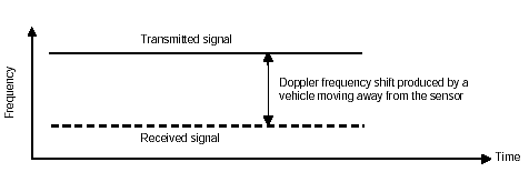
Figure 2-57. Constant frequency waveform.
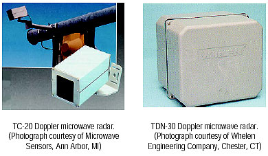
Figure 2-58. CW Doppler microwave radars.
Vehicle speed is proportional to the frequency change between transmitted and received signals in Doppler radars. The relation between the transmitted frequency f, Doppler frequency fD, and vehicle speed S is expressed as
 (2-64)
where θ is the angle between the direction of propagation of radar energy (i.e., the angle that represents the center of the antenna beam) and the direction of travel of the vehicle, c is the speed of light (3 x 10⁸ m/s), frequency is in units of Hz, and speed in units of m/s. The received frequency is given by f ± fD.(31)
The second type of microwave sensor used in traffic management and control applications transmits an FMCW waveform in which the transmitted frequency is constantly changing with respect to time, as depicted in Figure 2‑59a. The FMCW radar operates as a vehicle presence sensor and can detect motionless vehicles.
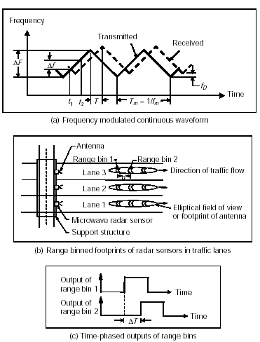
Figure 2-59. FMCW signal and radar processing as utilized to measure vehicle presence and speed
(Source: L.A. Klein, Sensor Technologies and Data Requirements for ITS (Artech House, Norwood, MA, 2001)).
The range R to the vehicle is proportional to the difference in the frequency ![]() f of the transmitter at the time t1 the signal is transmitted and the time t2 at which it is received, as given by
f of the transmitter at the time t1 the signal is transmitted and the time t2 at which it is received, as given by
 (2-65)
where
![]() f = instantaneous difference in frequency, in Hz, of the transmitter at the times the signal is transmitted and received
f = instantaneous difference in frequency, in Hz, of the transmitter at the times the signal is transmitted and received
![]() F = radio frequency (RF) modulation bandwidth in Hz
F = radio frequency (RF) modulation bandwidth in Hz
fm = RF modulation frequency in Hz.
Alternatively, the range may be calculated from t2 — t1 or from the time difference T between consecutive peaks in the received and transmitted signals as indicated in Figure 2-59a. The range R, in terms of t2 — t1 or T, is
 (2-66)
when the transmitter and receiver are collocated. The quantity c is the speed of light (3 x 10⁸ m/s).
The range resolution ![]() R or minimum distance, in meters, resolved by an FMCW radar is
R or minimum distance, in meters, resolved by an FMCW radar is
 (2-67)
Therefore, if the radar operates in the 10.500 to 10.550 GHz band and the bandwidth is limited to 45 MHz (rather than the full 50 MHz) to ensure that the field strength is reduced by at least 50 dB outside the band, the range resolution is at best 10.8 ft (3.3 m).
Speed or Doppler resolution ![]() fD is given by
fD is given by
 (2-68)
where Tm = 1/fm is the time for an up and down frequency sweep, as depicted in Figure 2-59a.
The FMCW radar measures vehicle speed by dividing the field of view in the direction of vehicle travel into range bins as shown in Figure 2-59b. A range bin allows the reflected signal to be partitioned and identified from smaller regions on the roadway. Vehicle speed S is calculated from the time difference ![]() T corresponding to the vehicle arriving at the leading edges of two range bins a known distance d apart as illustrated in Figure 2-59c. The vehicle speed is given by
T corresponding to the vehicle arriving at the leading edges of two range bins a known distance d apart as illustrated in Figure 2-59c. The vehicle speed is given by
 (2-69)
where
d = distance between leading edges of the two range bins
![]() T = time difference corresponding to the vehicle's arrival at the leading edge of each range bin.
T = time difference corresponding to the vehicle's arrival at the leading edge of each range bin.
When mounted in a side-looking configuration, multilane FMCW radar sensors can monitor traffic flow in as many as eight lanes. With the sensor aligned perpendicular to the traffic flow direction, the range bins are automatically or semiautomatically (depending on the sensor model) adjusted to overlay a lane on the roadway to enable the gathering of multilane traffic flow data. FMCW radars can also use Doppler to calculate the speed of moving vehicles. A discussion of this technique is beyond the scope of this Handbook, but can be found in References 19 and 37.
Presence-detecting radars, such as the models illustrated in Figure 2-60, control left turn signals, provide real-time data for traffic adaptive signal systems, monitor traffic queues, classify vehicles in terms of vehicle length, and collect occupancy and speed (multi detection zone models only) data in support of freeway incident detection algorithms. CW Doppler radars are used to measure vehicular speed on city arterials and freeways, but cannot detect stopped vehicles. Multi detection zone microwave presence-detecting radars are gaining acceptance in electronic toll collection and automated truck weighing applications that require vehicle identification based on vehicle length.
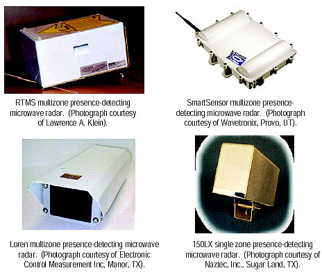
Figure 2-60. FMCW microwave radars. These are examples of microwave radars that detect vehicle presence.
Laser radar sensors have two sets of optics. The transmitting optics split the pulsed laser diode output into two beams separated by several degrees, as displayed in Figure 2-61. The receiving optics has a wider field of view so that it can better collect the energy scattered from the vehicles. The multiple beams allow laser radars to measure vehicle speed by recording the times at which the vehicle enters the detection area of each beam. Since the beams are a known distance apart, the speed is easily calculated from the familiar speed equals distance over time.
The laser radar illustrated in Figure 2-62 mounts 20 to 25 ft (6.1 to 7.6 m) above the road surface with an incidence angle (i.e., forward tilt) of 5 deg. A rotating polygon is utilized to line scan a laser diode rangefinder across the traffic lane as shown in Figure 2-61.(38) A sister model scans the laser across two lanes.(39) Their ability to classify 11 types of vehicles has found application on toll roads.
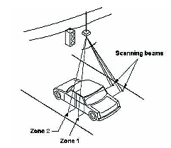
Figure 2-61. Laser radar beam geometry (drawing courtesy of Schwartz Electro-Optics, now OSI Laserscan, Orlando, FL).
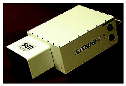
Figure 2-62. Autosense II laser radar sensor
(Photograph courtesy of Schwartz Electro-Optics, now OSI Laserscan, Orlando, FL).
Another commercial laser radar for collecting traffic flow data is shown in Figure 2-63. This model does not continuously scan the laser beam across a traffic lane. Instead it uses six individual pairs of transmitters and receivers to produce a beam that traverses the lane. The number of active transmitter-receiver pairs can be specified by the user to control the width of the laser scan across a single lane. The effective range of the device is up to 23 ft (7 m).
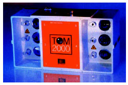
Figure 2-63. EFKON Traffic Observation Module (TOM) laser radar sensor (Photograph from EFKON product literature).
Active infrared sensors also communicate traffic information to motorists by modulating and coding the infrared beam with the appropriate data. Figure 2-64 depicts a sensor system used for this application.
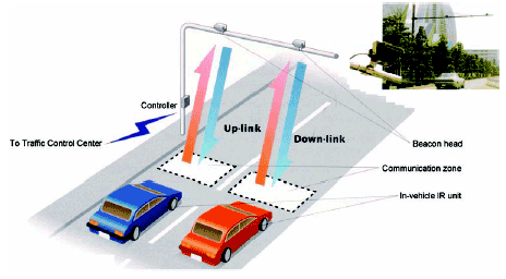
Figure 2-64. Active infrared sensor installed for transmitting traffic conditions to motorists
(Photograph courtesy of Sumitomo Electric U.S.A. Inc., Santa Clara, CA).
Passive sensors transmit no energy of their own. Rather they detect energy from two sources: (1) energy emitted from vehicles, road surfaces, and other objects in their field of view and (2) energy emitted by the atmosphere and reflected by vehicles, road surfaces, or other objects into the sensor aperture. The energy captured by passive infrared sensors is focused by an optical system onto an infrared-sensitive material mounted at the focal plane of the optics. With infrared sensors, the word detector takes on another meaning, namely the infrared sensitive element that converts the reflected and emitted energy into electrical signals. Real-time signal processing is used to analyze the signals for the presence of a vehicle. The sensors are mounted overhead to view approaching or departing traffic. They can also be mounted in a side-looking configuration. Infrared sensors are used for signal control; volume, speed, and class measurement; detection of pedestrians in crosswalks; and transmission of traffic information to motorists.
Nonimaging passive infrared sensors used in traffic management applications contain one or several (typically not more than five) energy-sensitive detector elements on the focal plane that gather energy from the entire scene. The detector in a nonimaging sensor generally has a large instantaneous field of view. Instantaneous field of view is equal to the angle, e.g., in the x-y plane, subtended by a pixel. Objects within the scene cannot be further divided into subobjects or pixels with this device.
Passive infrared sensors with a single detection zone measure volume and lane occupancy by responding to vehicle passage and presence. Those with multiple detection zones can also measure vehicle speed and length (to the extent that vehicles are detected in one or more detection zones a known distance apart). Imaging sensors, such as modern charge-coupled device (CCD) cameras, contain two-dimensional arrays of detectors, each detector having a small instantaneous field of view. The two-dimensional array gathers energy from the scene over an area corresponding to the field of view of the entire array. Imaging sensors display the pixel-resolution details characteristic of the imaged area, as illustrated in Figure 2-65.(40) An alternative method of gathering two-dimensional images is by scanning one-dimensional arrays over the scene of interest. However, this approach is not currently applied to passive infrared traffic flow sensors.
The emitted energy detected by passive sensors is produced by the nonzero surface temperature of emissive objects in their field of view. Emission occurs at all frequencies by objects not at absolute zero (-459.67 °F or -273.15 °C). If the emissivity of the object is perfect, i.e., emissivity = 1, the object is called a blackbody. Most objects have emissivities less than 1 and, hence, are termed graybodies. Passive sensors can be designed to receive energy at any frequency. Cost considerations make the infrared band a good choice for vehicle sensors with a limited number of pixels. Passive infrared sensors, such as those shown in Figure 2-66, operate in the long-wavelength infrared band from 8 to 14 mm and thus minimize the effects of sun glint and changing light intensity from cloud movement. Passive vehicle sensors operating at microwave frequencies have been evaluated, but their costs are greater.(40,41)
Figure 2-65. Visible spectrum CCD camera imagery of approaching traffic typical of dawn and dusk lighting (Source: C.A. MacCarley, B.M. Hemme, and L.A. Klein, Advanced Image Sensing Methods for Traffic Surveillance and Detection, Final Report, Document No. TEL5859F98 (Rev. 1) (California Polytechnic University, San Luis Obispo, CA, Jun. 30, 1998).
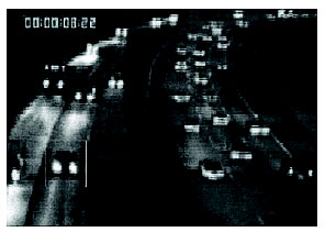
Figure 2-65
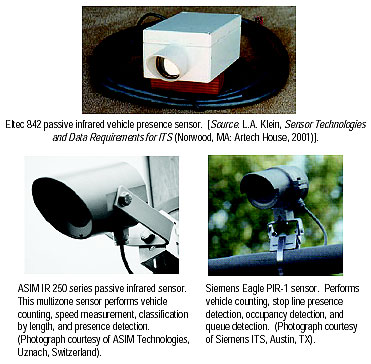
Figure 2-66. Passive infrared sensors
When a vehicle enters a passive sensor's field of view, the detected energy changes due to the presence of the vehicle. The difference in detected energy created by the vehicle is described by radiative transfer theory.(19,31,42) The emissivities of the vehicle and road surface in the wavelength region of interest are denoted by ![]() V and
V and ![]() R and their surface temperatures in degrees Kelvin by TV and TR, respectively, as depicted in Figure 2-67.
R and their surface temperatures in degrees Kelvin by TV and TR, respectively, as depicted in Figure 2-67.
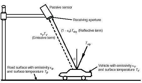
Figure 2-67. Emission and reflection of energy by vehicle and road surface.
The apparent temperature TBV of the vehicle is
 (2-70)
assuming infrared energy emission by the sensor is negligible. The sky temperature Tsky is a function of atmospheric, galactic, and cosmic emission. The atmospheric emission in the infrared spectrum is dependent on the water, ozone, carbon dioxide, nitrous oxide, and methane concentrations. The angles θ and Φ are the incident angle with respect to nadir (i.e., directly downward) and the angle in the plane of the road surface (the x-y plane), respectively. The term εVTV represents the energy emitted from the vehicle, referred to as the brightness temperature. The term (1 — εV) Tsky is the portion of the sky temperature that is reflected from the metal vehicle into the passive sensor. Thus, surfaces that are highly emissive (large ε) have a low reflective component (small 1 — ε).
One can also write an expression similar to Equation 2-70 for the apparent temperature of the road surface as
 (2-71)
The terms in Equation 2-71 have interpretations analogous to those in Equation 2-70. By subtracting the apparent temperature of the vehicle from that of the road, one gets an expression for the temperature difference ![]() TB (
TB (![]() ,
, ![]() ) sensed by the passive infrared sensor when a vehicle passes through its field of view. Thus
) sensed by the passive infrared sensor when a vehicle passes through its field of view. Thus
 (2-72)
When TV = TR, then
 (2-73)
Hence, a vehicle entering the sensor's field of view generates a signal that is proportional to the product of an emissivity difference term and a temperature difference term when the surface temperatures of the vehicle and road are equal. The emissivity term is equal to the difference between the road and the vehicle emissivities. The temperature term is equal to the difference between the absolute temperature of the road surface and the temperature contributed by atmospheric, cosmic, and galactic emission. On overcast, high humidity, and rainy days, the sky temperature is larger than on clear days and the signal produced by a passing vehicle decreases. This, in itself, should not pose a problem to a properly designed passive infrared sensor operating at the longer wavelengths of the infrared spectrum, especially at the relatively short operating ranges typical of traffic management applications.
Fields of view can be tailored through the optical design to accommodate different requirements such as stopline presence detection and presence detection in the approach to an intersection [e.g., a detection zone 68 to 100 ft (20.7 to 30.5 m) in advance of the stopline]. A long focal length lens eliminates adjacent lane detection when sensing vehicles over 100 ft (30.5 m) from the sensor, e.g., as they approach an intersection.
Multichannel (i.e., incorporating more than one type of sensor technology as in Figure 2-74) and multizone (i.e., including more than one detection region) passive infrared sensors measure speed and vehicle length as well as the more conventional volume and lane occupancy. These models are designed with dynamic and static thermal energy detection zones that provide the functionality of two inductive loops. Their footprint configuration is shown in Figure 2-68. The time delays between the signals from the three dynamic zones are utilized to measure speed. The vehicle presence time from the fourth zone is used to calculate the lane occupancy of stationary and moving vehicles.
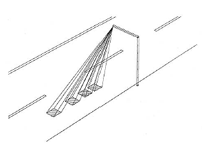
Figure 2-68. Multiple detection zone configuration in a passive infrared sensor.
Several disadvantages of infrared sensors are sometimes cited. Glint from sunlight may cause unwanted and confusing signals in passive sensors operating at near- or midinfrared wavelengths. Atmospheric particulates and inclement weather can scatter or absorb energy that would otherwise reach the focal plane. The scattering and absorption effects are sensitive to water concentrations in fog, haze, rain, and snow as well as to other obscurants such as smoke and dust. At the relatively short operating ranges encountered by infrared sensors in traffic management applications, these concerns may not be significant. However, some performance degradation (i.e., undercounting) in heavy rain and snow has been reported.(40) A rule of thumb for gauging when an infrared sensor may experience difficulty detecting a vehicle is to note if a human observer can see the vehicle under the same circumstances. If the observer can see the vehicle, there is a high probability the infrared sensor will detect the vehicle.
Ultrasonic sensors transmit pressure waves of sound energy at a frequency between 25 and 50 kHz, which are above the human audible range. Most ultrasonic sensors, such as the model shown in Figure 2-69, operate with pulse waveforms and provide vehicle count, presence, and occupancy information. Pulse-shape waveforms measure distances to the road surface and vehicle surface by detecting the portion of the transmitted energy that is reflected towards the sensor from an area defined by the transmitter's beamwidth. When a distance other than that to the background road surface is measured, the sensor interprets that measurement as the presence of a vehicle. The received ultrasonic energy is converted into electrical energy. This energy is then analyzed by signal processing electronics that is either collocated with the transducer or placed in a roadside controller.
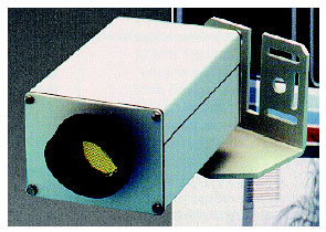
Figure 2-69. TC-30C ultrasonic range-measuring sensor
(Photograph courtesy of Microwave Sensors, Ann Arbor, MI).
Pulsed energy transmitted at two known and closely spaced incident angles allows vehicular speed to be calculated by recording the time at which the vehicle crosses each beam. Since the beams are a known distance apart, the speed can be calculated as beam separation distance divided by the time to traverse the beams. The preferred mounting configurations for range-measuring, pulsed ultrasonic sensors are at nadir, looking from an overhead position, and side viewing, as shown in Figure 2-70.
Constant frequency ultrasonic sensors that measure speed using the Doppler principle are also manufactured. However, these are more expensive than pulsed models. The speed-measuring Doppler ultrasonic sensor is designed to interface with the highway infrastructure in Japan. It is mounted overhead facing approaching traffic at a 45-deg incidence angle. It has two transducers, one for transmitting and one for receiving, as illustrated in Figure 2-71. The Doppler ultrasonic sensor detects the passage of a vehicle by a shift in the frequency of the received signal. Vehicle speed can be calculated from the pulse width of an internal signal generated by the sensor's electronics that is proportional to the speed of the detected vehicle.
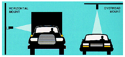
Figure 2-70. Mounting of ultrasonic range-measuring sensors
(Illustration courtesy of Microwave Sensors, Ann Arbor, MI).
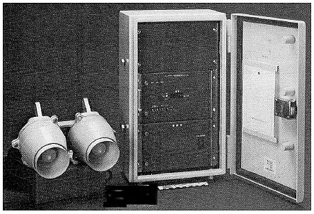
Figure 2-71. Speed-measuring RDU-101 Doppler ultrasonic sensor (manufactured by Sumitomo Electric, Japan) with separate transmitting and receiving transducers, as shown in the left portion of the figure. The cabinet on the right contains the electronic systems needed to supply power and control signals to the transducers, receive the data, and interface with the highway infrastructure.
The range-measuring ultrasonic sensor transmits a series of pulses of width Tp (typical values are between 0.02 and 2.5 ms) and repetition period T0 (time between bursts of pulses), typically 33 to 170 ms, as illustrated in Figure 2-72. The sensor measures the time for the pulse to arrive at the vehicle and return to the transmitter. The receiver is gated on and off with a user-adjustable interval that differentiates between pulses reflected from the road surface and those reflected from vehicles. The detection gates of various models are adjusted to detect objects at distances greater than approximately 0.5 to 0.9 m above the road surface. This is achieved by closing the detection gate several milliseconds before the reflected signal from the road surface arrives at the sensor.
Automatic pulse repetition frequency control reduces effects of multiple reflections and improves the detection of high-speed vehicles. This control makes the pulse repetition period as short as possible by transmitting the next pulse immediately after the reflected signal from the road is received.(43) A hold time Th (composite values from manufacturers range from 115 ms to 10 s) is built into the sensors to enhance presence detection.
Ultrasonic sensors are widely used in Japan in keeping with the government policy that discourages pavement cutting on existing highways. In Tokyo, ultrasonic sensors are a major component of the traffic control system. A central computer monitors traffic signals and vehicle motion, resets timing patterns, activates motorist information displays, and relays real-time information to motorists and police. The presence or range-measuring type of sensor is used more extensively than the Doppler type. The Japanese applications appear to be the most extensive use of ultrasonic sensors.
Temperature change and extreme air turbulence may affect the performance of ultrasonic sensors. Temperature compensation is built into some models. Large pulse repetition periods may degrade occupancy measurement on freeways with vehicles traveling at moderate to high speeds as an insufficient number of pulses is transmitted and reflected from the vehicle while in the sensor's detection zone.
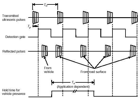
Figure 2-72. Operation of range-measuring ultrasonic sensor.
Acoustic sensors measure vehicle passage, presence, and speed by detecting acoustic energy or audible sounds produced by vehicular traffic from a variety of sources within each vehicle and from the interaction of vehicle's tires with the road. When a vehicle passes through the detection zone, an increase in sound energy is recognized by the signal processing algorithm and a vehicle presence signal is generated. When the vehicle leaves the detection zone, the sound energy level drops below the detection threshold, and the vehicle presence signal is terminated. Sounds from locations outside the detection zone are attenuated.
Single lane and multiple lane models of acoustic sensors are marketed. Both use a two-dimensional array of microphones to detect the sounds produced by approaching vehicles.
The SmartSonic acoustic sensor, shown in the upper part of Figure 2-73, detects vehicles by measuring the time delay between the arrival of sound at the upper and lower microphones, which are arranged in a vertical and horizontal line through the center of the aperture. The time delay changes as the vehicle approaches the array. When the vehicle is inside the detection zone, the sound arrives almost instantaneously at the upper and lower microphones. When the vehicle is outside the detection zone, sound reception at the upper microphone is delayed by the intermicrophone distance.
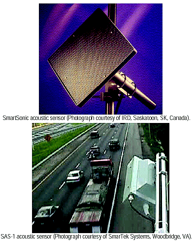
Figure 2-73. Acoustic array sensors.
The size and shape of the detection zone are determined by the aperture size, processing frequency band, and installation geometry of the acoustic array. The SmartSonic sensor is tuned to a center frequency of 9 kHz with a 2 kHz bandwidth. Preferred mounting is at 10 to 30 deg from nadir with a detection range of 20 to 35 ft (6 to 11 m).
The speed of a detected vehicle is determined with an algorithm that assumes an average vehicle length. Vehicle presence detection is through an optically isolated semiconductor. A serial interface on the controller card installed with the sensor provides volume, lane occupancy, speed, vehicle classification (cars, light trucks, heavy trucks, and buses), and sensor status messages. When the optional acoustic sensor controller board is installed in a NEMA or 170 cardfile, two detection zones can be used in a speed trap mode to measure vehicle speed. The speed trap activates relay outputs that simulate two inductive loops connected to a NEMA or 170 controller. The SmartSonic is recommended for data collection applications on bridges and other roads where nonintrusive sensors are required, providing either slow moving vehicles (speeds < 20 mi/h (32 km/h)) in stop-and-go traffic flow or free-flow traffic is present. The sensor is not recommended where a mix of stop-and-go and free-flow traffic occurs, such as on a freeway with the potential for congestion, because the vehicle detection algorithm cannot switch between these two flow conditions fast enough to detect the onset of the change in flow.
The SAS-1 acoustic sensor in the lower part of Figure 2-73 utilizes a fully populated microphone array and adaptive spatial processing to form multiple detection zones. The SAS-1 is designed to monitor up to 5 lanes when mounted in a side-looking configuration. During setup, the detection zones are steered to positions that correspond to the monitored traffic lanes. The detection zones are self-normalized and polled for vehicles every 8 ms. Detection zones are adjustable to 6 ft (1.8 m) or 12 ft (3.6 m) in the direction of traffic flow and have user-specified values in the cross-lane direction. Acoustic frequencies between 8 and 15 kHz are processed by this sensor, which accommodates mounting heights of 20 to 40 ft (6 to 12 m). The output data are volume, lane occupancy, and average speed for each monitored lane over a user-specified period (e.g., 20 s, 30 s, 1 minute). Vehicle presence is provided by an optional relay interface.
Figure 2-74 illustrates sensors that combine passive infrared presence detection with ultrasound or CW Doppler microwave radar.(44) The passive infrared-ultrasonic combination, shown in the upper portion of the figure, provides enhanced accuracy for presence and queue detection, vehicle counting, and height and distance discrimination.
The passive infrared-CW Doppler radar sensor, in the lower portion of the figure, is designed for presence and queue detection, vehicle counting, speed measurement, and length classification. It relies on the radar to measure high to medium vehicle speeds and the passive infrared to measure vehicle count and presence. At medium speeds, the multiple detection zone passive infrared automatically calibrates its speed measurements against the radar's. This calibration permits the infrared to measure slow vehicle speeds and detect stopped vehicles.
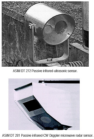
Figure 2-74. Passive infrared combination sensors (Photographs courtesy of ASIM Technologies, Uznach, Switzerland).
Previous | Table of Contents | Next
FHWA-HRT-06-108

