U.S. Department of Transportation
Federal Highway Administration
1200 New Jersey Avenue, SE
Washington, DC 20590
202-366-4000
Federal Highway Administration Research and Technology
Coordinating, Developing, and Delivering Highway Transportation Innovations
 |
| This report is an archived publication and may contain dated technical, contact, and link information |
|
Publication Number: FHWA-HRT-06-108
Date: May 2006 |
This chapter discusses the design of vehicle detection systems that use inductive-loop detectors, magnetometers, and magnetic detectors for surface street and freeway traffic management, with primary emphasis on inductive loops. The guidelines provided should serve traffic engineers in developing plans and specifications for vehicle detection at local intersections, detectorization for traffic signal systems, and freeway surveillance and control. Above-roadway sensors, such as those described in chapter 2, may also be an option for many of the applications discussed in this chapter.
When an in-roadway sensor is required for vehicle detection in a particular application, the first step in the design process is to determine what type of in-roadway sensor will supply the needed data or provide the required functionality. Some agencies have predetermined policies or standard plans that assist in the sensor selection process. To be effective, the standard plans should be updated to reflect current state of the practice in sensor and data transmission technology. Where standard plans are not appropriate or are not available, the following criteria may be applied as guidelines for in-roadway sensor selection.
Sensor selection for a specific traffic management application depends on the data parameters, data accuracies, spatial resolution, detection area, appropriate data transmission media, location-specific installation requirements, initial sensor cost, and the acceptability of the maintenance burden it will impose. These criteria, separately and in combination, should be assessed as part of the sensor selection process.
Sensor technology and operating theory described in chapter 2 indicate that the principal in-roadway sensors (inductive-loop, presence-detecting magnetometers, and passage-detecting magnetometers (also referred to as magnetic detectors)) are suitable for some applications, but unsuitable for others. For example, magnetometers cannot be used with NEMA controllers where delayed-call capability is required, since this feature is not available in magnetometers. In Type 170 controllers, the controller performs the timing operation; therefore, magnetometers can be used with 170 and the newer 2070 controllers. Search coil magnetometers must be excluded for operations requiring presence detection because they are only capable of detecting a moving vehicle (passage detection).
Inductive-loop detectors are not always appropriate for some traffic signalization applications. For example, long loops are not suitable for detection of oversaturated flow or long queues. Loops can be utilized for freeway surveillance and control if the area of the induced magnetic field is tailored to provide vehicle detection in the lane of interest and the time required for output, pick-up, and drop-out are predictable.
Applying lessons learned from the extensive application of in-roadway sensors further narrows sensor selection. In theory, both the inductive-loop detector and one or more presence-detecting magnetometers are suitable for large area detection on an approach to a signalized intersection. The loop detector, however, is usually less expensive. Conversely, for an approach where it is not important to screen out false calls for the green (i.e., right turns on red) and only rudimentary traffic detection is needed, any of the three in-roadway sensor types may be installed. In this particular application, the passage-detecting magnetometer might be favored because of its ruggedness and low cost/useful life ratio.
In the 1960s-1970s, it was common for large cities such as New York, NY, or Atlanta, GA, to select microwave radar or ultrasonic sensors because they could be installed on a suitable pole already in place and not disrupt traffic or break the pavement. A crew could install one of these sensors in about 45 minutes. Recent advances in over-roadway sensor design have encouraged a new interest in these sensors and other over-roadway sensor technologies such as video image processors and laser radars.
Today, agencies often look favorably on eliminating a saw cut or replacing it with a drilled hole. The pervasiveness of deteriorating pavements has produced more interest in installing preformed loops, microloops, or pavement slabs with sensors already in place. Another approach to eliminating saw cuts is to install preformed loops or prewound loops in conjunction with repaving. Chapter 5 describes some of the approaches that simplify installation of in-roadway sensors.
Most traffic engineering agencies are aware of the cost differences in maintaining sensors based on different operating technologies. For example, the passage-detecting magnetometer detector, with its limited application, has managed to retain some popularity largely because of its ruggedness and long life with minimum maintenance. The improved reliability and functionality in inductive-loop detector electronics units have shifted the main sources of loop detector failure to the wire loop in the pavement, its connection to the lead-in cable, and loop installation issues. The requirement for more rugged loop detector installations has highlighted the need for reduced maintenance costs in terms of frequency of failures and resulting maintenance calls. Chapter 6 discusses these issues further.
Sensor selection for vehicle detection at intersections is a function of the types of timing intervals generated by the controller and the corresponding data needed to compute the intervals. Therefore, the timing interval types should be selected early in the traffic signal control design process. Similar considerations apply to the design of freeway signal control strategies. The following discussion defines various timing parameters, effect of short-loop and long-loop configurations, and detection alternatives for low-speed and high-speed approaches.
An actuated phase normally has three timing parameters in addition to the yellow change and all-red clearance intervals. These are the minimum green (also known as initial interval), the passage time (also called the vehicle interval, extension interval, or unit extension), and the maximum interval.(1) Relationships among the intervals are shown in Figure 4-1. These intervals are timed depending on the type and configuration of the sensor installation found at the intersection.
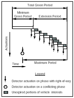
Figure 4-1. Actuated controller green phase intervals.
The majority of early vehicle sensors were point detectors consisting of treadles or pressure plates in the roadway. Today's 6- x 6-ft (1.8- x 1.8-m) inductive-loop detector also performs as a point detector. With point detection, the minimum green interval is set to allow vehicles stopped between the detection point and the stopline to start and move into the intersection. Table 4-1 shows the minimum green interval for various distances from the stopline. The data are based on an average vehicle headway distance of 20 ft (6 m) and the average times for vehicles from a queue to enter the intersection.
Distance between stopline and sensor |
Minimum green time |
|
|---|---|---|
feet |
meters |
seconds |
0–40 |
0–12.2 |
8 |
41–60 |
12.5–18.3 |
10 |
61–80 |
18.6–24.4 |
12 |
81–100 |
24.7–30.5 |
14 |
101–120 |
30.8–36.6 |
16 |
A different timing approach is used to establish minimum green intervals for presence detection. When long loops (or a series of short loops) that terminate at the stopline are used, the initial interval is set as small as zero seconds to achieve "snappy" response for left-turn phases or possibly longer for through movements where drivers may expect a longer green. If the loop ends some distance from the stopline, this distance is used to calculate the interval time in the same way as for point detection.
The passage time interval is calculated such that a vehicle can travel from the sensor to the intersection. This is particularly important where point detection is used and the sensors are located some distance from the stopline. The passage time also defines the maximum apparent time gap between vehicle actuations that can occur without losing the green indication to a call waiting. As long as the interval between vehicle actuations is shorter than the passage time, the green will be retained on that phase (subject to the maximum green interval described in the following section).
The apparent time gap for a single stream of vehicles passing over an inductive-loop detector is somewhat shorter than the actual time gap. A vehicle activates the loop upon entry over the loop, and the loop does not deactivate until the vehicle leaves the loop. The true time gap is reduced by the time it takes the vehicle to traverse the loop.
Another factor in determining an appropriate vehicle interval is the number of approach lanes containing sensors. Inductive-loop detectors for the same phase and function installed in adjacent lanes are often connected to the electronics unit by a single lead-in cable. This may introduce errors into the number of vehicles reported.
NEMA controllers identified as "advanced design," "exceeds," or "beyond" have a predefined minimum green time. If no further actuations occur, the minimum green is the total green. If there are further actuations, the passage time interval extends the green until a gap exceeds the passage time or the maximum green time is reached. The relationship of these times was illustrated in Figure 4-1.
When long loops are used in approaches, especially in left turn bays, the minimum green and the passage time intervals are generally set to zero or near zero. The long loop operates in the presence mode and the controller continuously extends the green as long as the loop is occupied. The critical gap is not a preset value, but a space gap equal to the length of the loop. Thus, the gap length is equivalent to no following vehicle entering the loop prior to the departure of the previous vehicle.
When a series of short loops is utilized, it acts as a single long loop, provided the space between loops is less than a vehicle length. If the spacing is greater than a vehicle length, a short vehicle interval can be used to provide the same effect as a single long loop.
The maximum green interval limits the time a phase can hold the green. The maximum green begins timing at the first call received from an opposing (or conflicting) phase. Ordinarily, maximum intervals for through movements are set between 30 and 60 seconds. When the signal is properly timed with appropriately short passage times (i.e., vehicle intervals), the maximum interval will not consistently time out unless the intersection is badly overloaded. Some actuated controllers are capable of providing two maximum intervals per phase. This allows longer maximums to be programmed during peak periods (or shorter maximums for selected phases) when very heavy traffic flows are expected on the major street.
Volume-density phases have more timing parameters than a standard actuated phase. For this type of operation, sensors are generally placed further back from the intersection, particularly on high-speed approaches. The minimum green interval can be increased to provide longer initial green times for those instances when the minimum green is not adequate to serve the actual traffic present. The length of the initial green interval is governed by three factors—minimum green, seconds per actuation, and maximum initial—as described by the timing procedure illustrated in Figure 4-2. The variable initial interval is described by NEMA Standards in the following paragraph:(2)
In addition to MINIMUM GREEN, PASSAGE TIME, and MAXIMUM GREEN timing functions, phases provided with VOLUME DENSITY operation shall include VARIABLE INITIAL timings and GAP REDUCTION timings. The effect on the INITIAL timing shall be to increase the timing in a manner dependent upon the number of vehicle actuations stored on this phase while its signal is displaying YELLOW or RED. The effect on the extensible portion shall be to reduce the allowable gap between successive vehicle actuations by decreasing the extension time in a manner dependent upon the time waiting of vehicles on an opposing RED phase.
In volume-density phases, the extended green time (passage time) created by each new actuation after the initial green time has elapsed is normally based on the time required to travel from the sensor to the stopline. Because this distance can be relatively long, the passage time can be more than the desired allowable gap. The NEMA gap reduction procedure addresses this situation. It defines four time settings—time before reduction, passage time, minimum gap, and time to reduce, as illustrated in Figure 4-3. The time before reduction begins when there is a call on a conflicting phase. Once the time before reduction has expired, the allowable gap reduces linearly until the minimum gap is reached at the end of the time-to-reduce interval. The maximum green extension and yellow change and all-red clearance intervals are predetermined (precalculated) and programmed into the controller.
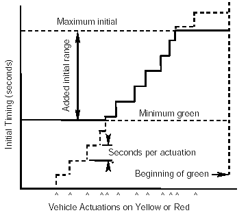
Figure 4-2. Variable initial NEMA timing for green signal phase.
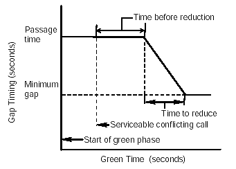
Figure 4-3. NEMA gap reduction procedure.
Approaches with speeds of less than 35 mi/h (55 km/h) are considered low-speed approaches. The sensor design for a given approach depends on whether the controller phase has been set for locking or nonlocking detection memory. This is also referred to as memory ON or memory OFF. The locking feature means that a vehicle call for the green is remembered or held by the controller until the call has been satisfied by the display of the green indication, even if the calling vehicle has left the detection area (e.g., right turn on red). In the nonlocking mode, the controller drops a waiting call as soon as the vehicle leaves the detection area.
Locking detection memory is associated with the use of small-area point sensors such as a 6- x 6-ft (1.8- x 1.8-m) inductive loop and is frequently referred to as conventional control. The minimum green interval (or initial interval) is preset to provide sufficient time to clear a standing queue between the sensor and the stopline. The passage time or unit extension sets a common value for both the allowable gap to hold the green and the travel time from sensor to stopline.
Since the allowable gap is usually 3 or 4 seconds, the sensor might be ideally located 3 or 4 seconds of travel time upstream from the intersection. This sensor position would appear to be the most efficient for accurately timing the end of green after passage of the last vehicle of a queue. However, a long minimum green (assured green) is created at approaches with speeds greater than 25 to 30 mi/h (40 to 50 km/h) because of the longer sensor setback. Therefore, the principle is amended to locate sensors 3 to 4 seconds of travel time from, but not more than 170 ft (52 m), from the stopline. Some agencies limit this distance to 120 ft (37 m). Table 4-2 displays the application of this principle to determining sensor location and associated timing parameters as a function of vehicle approach speed.
Approach speed |
Detector setback from stopline to leading edge of inductive-loop detector |
Minimum green time |
Passage time |
||
|---|---|---|---|---|---|
mi/h |
km/h |
feet |
meters |
seconds |
seconds |
15 |
24 |
40 |
12 |
9 |
3.0 |
20 |
32 |
60 |
18 |
11 |
3.0 |
25 |
40 |
80 |
24 |
12 |
3.0 |
30 |
48 |
100 |
30 |
13 |
3.5 |
35 |
56 |
135 |
41 |
14 |
3.5 |
40 |
64 |
170 |
52 |
16 |
3.5 |
45+ |
72+ |
Volume-density or multiple inductive-loop detectors recommended. | |||
Note: Volume-density could be considered at speeds of 35 mi/h (56 km/h) or above.
The advantage of this single sensor approach is that the cost of installation is minimized. However, this type of control does not screen out false calls for green as occurs with right turns on red.
Nonlocking detection memory is used with larger-area sensors such as a 6- x 50-ft (1.8- x 15.2-m) loop. Often called loop occupancy control, the technique requires a nominal loop configuration as shown in Figure 4-4. The vehicle presence information provided in the area near the intersection allows the elimination of many of the false calls for green and thus avoids unnecessary green signals in approaches with no waiting vehicles. The disadvantages of this traffic control method are the higher initial cost of sensor installation and the higher replacement and maintenance costs associated with larger inductive-loop detectors.
Nonlocking detection memory is particularly appropriate in left-turn lanes with separate signal control for the left turns. The green arrow is terminated as soon as the turning vehicle clears the loop. In addition, a call placed during the yellow change interval by a vehicle that clears on the yellow does not bring back the green to an empty approach. Another potential advantage occurs when the left turn is permitted. In this case, the left turn is allowed to filter across oncoming traffic on the circular green shown to the through movement. Accordingly, left turns may be serviced during the through phase and, therefore, do not require the display of a left arrow.
Figure 4-4. Intersection configured for loop occupancy control.
The left turn bay may use an electronics unit operating in a delayed-call mode, which is designed to send an output to the controller only if a vehicle is continuously detected beyond a preset period (e.g., 5 seconds). This allows the electronics unit and controller to ignore vehicles that are in transit over the loop if oncoming traffic is light enough to allow a left turn without the protective left-turn arrow. If oncoming traffic is so heavy that left turning vehicles queue up over the loop, then the green arrow is called. This type of controller operation is often used with lagging left-turn phasing.
A similar operation occurs on a single lane approach from the cross street where a right-turning vehicle approaches on the red. Again, the use of a delayed call electronics unit will avoid calling the green to the side street if the right turn on red can be made during the delay time set on the electronics unit.
Loop-occupancy control is also utilized for through lane control on low-speed approaches. The technique minimizes delay by allowing short passage times (unit extensions) in the range of 0 to 1.5 seconds. The length of the detection zone obviously depends on the approach speed and the controller unit time settings. Figure 4-5 gives the length of the long-loop presence detector for various passage time settings on the controller for approach speeds less than 30 mi/h (50 km/h). The figure is based on a desired allowable gap of 3 seconds and an average vehicle length of 18 ft (5.5 m). The formula for loop length is
![]() (4-1a)
(4-1a)
![]() (4-1b)
(4-1b)
where
L = length of detection area, ft (m)
S = approach speed, mi/h (km/h)
PT = passage time (unit extension),seconds.
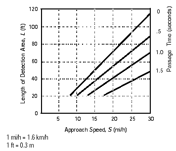
Figure 4-5. Inductive-loop detector length for loop occupancy control.
Approaches with speeds in excess of 35 mi/h (56 km/h) are considered high-speed approaches. Several problems associated with high-speed approaches require special consideration in setting signal timing intervals. For example, it may be difficult for the driver to decide whether to stop or proceed when approaching a yellow change indication. An abrupt stop may result in a rear-end collision, while the decision to proceed through the intersection may cause a right-angle accident or a traffic violation.
The portion of the roadway in advance of the intersection in which the driver is indecisive (as to stopping or proceeding into and through the intersection at the onset of the yellow change interval) is called the dilemma zone. Some researchers have defined the dilemma zone as that area of the approach between a point where 90 percent of the drivers will stop on yellow and a point where 90 percent of the drivers will go (i.e., 10 percent will stop).(3,4) Table 4-3 shows these boundaries for various speeds.
Approach speed |
Distance from intersection for 90% probability of stopping |
Distance from intersection for 10% probability of stopping |
|||
|---|---|---|---|---|---|
mi/h |
km/h |
feet |
meters |
feet |
meters |
35 |
56 |
254 |
77 |
102 |
31 |
40 |
64 |
284 |
87 |
122 |
37 |
45 |
72 |
327 |
100 |
152 |
46 |
50 |
80 |
353 |
108 |
172 |
52 |
55 |
88 |
386 |
118 |
234 |
71 |
Figure 4-6 illustrates the dilemma zone for a vehicle approaching an intersection at 40 mi/h (64 km/h). To minimize the untimely display of yellow and thus the creation of a dilemma zone problem, a number of techniques have been devised for controllers with locking and nonlocking detection memory, basic actuated and volume-density controller circuitry, and various inductive-loop detector configurations.
The most straightforward conventional design for a high-speed approach utilizes a controller with a volume-density mode. This type of actuated operation can count waiting vehicles beyond the first because of the added initial feature. It also has a timing adjustment to reduce the allowable gap based on the time vehicles have waited on the red on a conflicting phase.
More efficient operation can be achieved with the volume-density mode than with fully actuated control because of the added initial and timing adjustment features and because detection is farther back on the approach— 400 ft (120 m) is typical. A calling sensor near the stopline that operates only when the phase is red or yellow often supplements high-speed approach detection. This calling sensor is disabled when the signal turns green so that it cannot extend the green time inappropriately.
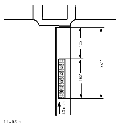
Figure 4-6. Dilemma zone for vehicle approaching an intersection at 40 mi/h (64 km/h).
Fully-actuated controllers utilizing an extended-call sensor just upstream of the dilemma zone have been in service since at least 1982. Designs for high-speed approaches using nonlocking detection memory include a long loop at the stopline as well as one or more small loops upstream. The long loop improves the controller's knowledge of traffic at the stopline, but tends to increase the allowable gap.
Inductive-loop designs for both normal fully actuated and volume-density controllers are available. Additional information concerning these solutions to the dilemma zone problem is presented later in this chapter.
For isolated high-speed rural intersections, a "PREPARE TO STOP" extinguishable message sign is frequently deployed when the signal site undergoes periods of poor visibility caused by dense ground fog, orientation of the sun, or geometry that prevents signal visibility far enough in advance to ensure safety. These situations require vehicle sensors further in advance of the intersection than normal.
Using the last car passage feature of some density controllers, the gap in the traffic flow can be identified to allow the last car in the platoon to pass through the signal and presumably give the next vehicle sufficient time to stop. The message sign, such as the one depicted in Figure 4-7, would flash PREPARE TO STOP at the appropriate time, but would be blank or unreadable at other times.
When the controller is informed of a gap in the traffic, it does not change the signal until a preset time has elapsed to allow the last car to clear the intersection. The PREPARE TO STOP is illuminated when the gap is selected, so that the next vehicle following the platoon will see the sign. Thus, the driver will know he will be required to stop even though the signal ahead is still green.
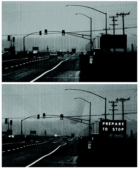
Figure 4-7. PREPARE TO STOP sign on an arterial in nonilluminated and illuminated states.
A typical inductive-loop detector and sign placement layout for a PREPARE TO STOP installation is shown in Figure 4-8. A display used by some jurisdictions consists of flashing beacons together with a diamond or rectangular sign with the message PREPARE TO STOP WHEN FLASHING.
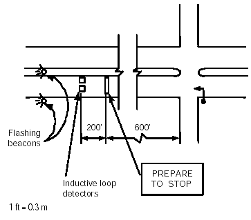
Figure 4-8. PREPARE TO STOP inductive-loop detector system.
The commuting driver frequently uses residential roadways as a time-saving route for reaching destinations, particularly when the residential street is parallel to a congested arterial. Residents generally perceive the added commuter traffic as a threat to the safety of children, pets, and their ability to safely exit their driveways, particularly where speeding occurs.
To control traffic speeds in residential areas, traffic engineers have used a variety of traffic control devices such as stop signs, warning signs, speed bumps, and coordinated traffic signals with vigorous enforcement of posted speed limits. While these measures are often successful, there are drawbacks associated with their use.
For example, the use of unwarranted stop signs to control vehicular speeds imposes delay penalties on all drivers, and it only affects speeds within 200 ft (60 m) of the stop sign. Unwarranted stop signs may also encourage drivers to ignore the stop sign, which is even more dangerous.
One approach for slowing speeding vehicles is to install two speed-measuring inductive-loop detectors (or other sensor types) approximately 180 ft (55 m) in advance of the intersection. The advance loops measure the speed (through measurement of the elapsed time to travel between the loops) of an approaching vehicle and register a call on the controller only if the vehicle is traveling at or below the speed limit. Assuming the signal is resting in four-way red and the vehicle is not speeding, a green is displayed and the driver may proceed through the intersection without being delayed. If, on the other hand, the approaching vehicle is exceeding the speed limit, no call is placed and the driver must slow down until he reaches a loop near the intersection. A call will then be placed and the green interval activated.
Consequently, the timing cycle to initiate a call begins when a vehicle crosses the first advance loop. If the vehicle speed is low enough, the predetermined interval will time out before the vehicle reaches the second loop. Then the call request will be passed to the controller. When the vehicle reaches the second loop, the timing device is reset, and any call being held at the timing device is cancelled. Thus, a vehicle exceeding the speed limit is never detected by the advance loop, and each succeeding vehicle is timed independently. This method is simple, economical, adjustable, and not dependent on vehicle size or length.
The spacing between the initiating and resetting advance loops is approximately 1 second of travel distance at the speed limit. The distance from the advanced loop to the first intersection loop is predetermined from the lowest travel speed to be accommodated (normally 20 mi/h (32 km/h)) and the maximum desirable passage time interval (4 seconds). A comfortable reaction time and the stopping distance at the design speed determine the minimum distance from a stopline to the advance detector loop.
Small-area (for point or passage detection) and larger-area (for area or presence detection) inductive-loop detector design is described in this section. Passage-detecting search coil magnetometers (magnetic detectors) can only be used for point detection because they are sensitive to vehicles in small areas and require vehicle motion (passage) for activation. Presence-detecting two-axis fluxgate magnetometers are also point detectors, but can be used as area detectors by using multiple sensors to cover a larger area.
Typical design configurations for sensor locations in through lanes and in left-turn lanes are also presented. Both simple and complex designs are described along with the type of controller operation, if appropriate. Treatments to alleviate the dilemma zone problem are also discussed.
Small-area detection is commonly implemented with a single short inductive loop. Although the literature defines short loops as being up to 20 ft (6.1 m) in length, by far the most common short-loop application is the 6- x 6-ft (1.8- x 1.8-m) loop in a 12-ft (3.6-m) lane. For narrower lanes, 5- x 5-ft (1.5- x 1.5-m) loops should be used to avoid adjacent lane pickup (splashover). Smaller loops are not recommended in areas where high-bed vehicles must be continuously detected.
The short loop is intended to detect a vehicle upstream of the stopline. When a vehicle passes over the loop, a call is output by the electronics unit to the controller. Timing of the green interval is commonly based on preset controller settings, not by the length of time the detection area is occupied by vehicles approaching the intersection. In most cases, the controller operates with locking detection memory circuits to insure calling the appropriate phase.
Short-loop detectors may be used in a variety of ways and may be located at varying distances from the stopline, depending on the operational requirements. A typical application may consist of one or more short loops near the stopline on the actuated approach of a low-speed intersection. Another typical application is to space a number of these loops well back of the stopline to act as extension sensors for higher-speed approaches.
Loop shapes were the subject of a great amount of research during the l970s and 1980s. Subsequently, many loop configurations were designed to detect the various sizes and shapes of vehicles that travel on the Nation's roadways, from bicycles and motorcycles to high-bed trailer trucks, while avoiding detection of vehicles in adjacent lanes. Each design purports to have advantages over other designs. Examples of short loop shapes are illustrated in Figure 4-9. Some of these configurations are common, while others are found at either a site-specific location or when particular types of vehicles require detection.
Figure 4-9. Small loop shapes.
A number of agencies and universities have conducted tests to determine an optimum loop shape.(5,6,7) These projects typically involved installing several different loop shapes and then testing and comparing the sensitivity of the loops in detecting several types of test vehicles. None of these projects tested all of the loop designs currently in use. In some cases, one loop design would test better when compared to one or two different loop designs. In most instances, the difference in sensitivity among loops was not significant, given the state of the art in electronics units. It is therefore difficult to cite one particular design as superior to all others. However, it is generally accepted that some loop designs are better suited than others for detecting small vehicles or high-bed trucks, as discussed in later sections.
Many States specify the acceptable loop shapes for use in their jurisdiction. An example is Caltrans's specified shapes shown in Figure 4-10. In this particular example, each unique shape is given a letter designation (e.g., type A is the conventional 6- x 6-ft (1.8- x 1.8-m) loop).
Larger-area detection normally contains a detection zone covering an area of at least 20 ft (6 m) or more in a traffic lane. It is primarily used for presence detection because the detection zone registers the presence of a vehicle as long as the zone is occupied. This concept originally used a single loop encompassing the entire detection zone. However, the long loop, as a single entity, is being supplanted by a sequence of short loops, which emulate the long loop. In this Handbook, the term long loop means either a single long loop or multiple short loops functioning as a single long loop.
Figure 4-10. Caltrans-specified loop shapes.
Figure 4-11 illustrates the traditional long loop (i.e., a single loop 6 ft (1.8 m) wide by 20 to 80 ft (6 to 24 meters) long or longer) and other long-loop shapes. These long loops generally have only one or two turns of wire. If the rectangular, powerhead or trapezoidal loop needs to reliably detect all roadway vehicles, the sensitivity level must be set high which, in turn, causes detection of adjacent lane vehicles (splashover). The quadrupole loop is an appropriate design to eliminate this problem. However, due to its limited field height, it may have difficulty in continuously detecting high-bed vehicles. Quadrupoles are excellent wheel and axle sensors. The lengths associated with long loops increase the vulnerability to failure caused by pavement cracks and joint movement. In response to these problems, many agencies are installing sequential short loops.
The long loop normally provides input to the controller for operating in the loop occupancy mode. In this control mode, the minimum green interval (or initial interval in older controllers) is set to zero or near zero, and the passage time or vehicle interval is set to a small value, as was shown in Figure 4-5. When the green interval appears for the subject phase, it remains green as long as the loop is occupied (subject, of course, to the maximum green). As soon as the inductive-loop detector is cleared, the passage time is measured and, if no further actuation occurs during the passage time, the yellow change interval appears.
Figure 4-11. Long loop shapes
The effective time gap is equal to the travel time required to traverse the length of the loop plus one vehicle length plus the passage time. Thus, the length of the loop is a critical measure for providing appropriate operation. The length must be sufficient for a following car to come to a stop if the yellow interval appears just before the following vehicle reaches the loop or, conversely, to allow the vehicle to proceed through the intersection on the yellow.
If heavy trucks are included in the traffic stream, there may be a start-up issue if a long queue exists. Passenger cars in front of the truck may accelerate and clear the inductive-loop detector before the truck can accelerate and reach the detector.
One researcher examined the relationship between inductive-loop detector length and the time settings of vehicle interval and maximum green for intersections where vehicle approach speeds were less than 35 mi/h (56 km/h).(8) The purpose of the study was to determine the optimal combinations of loop length, vehicle interval, and maximum green for a wide range of flow conditions (i.e., flow rate per lane, distribution of traffic among lanes, and temporal variations in flow rates). Both two- and four-phase operation of presence mode control were analyzed for each flow pattern.
Optimal vehicle intervals are a function of inductive-loop detector length and flow rate. The study suggests that for loops 30 ft (9 m) long, the use of 2-second vehicle intervals can lead to the best signal performance over a wide range of operating conditions. For 50-ft (15-m) loops, 1-second vehicle intervals are desirable under a variety of flow conditions. When loops 80 ft (25 m) long are used, 0-second vehicle intervals can minimize delays. Longer vehicle intervals for such loop lengths are not desirable unless the combined critical flow at an intersection exceeds 1,400 v/h.
The study concluded that maximum green for presence-mode control is generally longer than optimal green durations for pretimed control. Flow patterns characterized by a larger concentration of traffic in short periods of time need longer maximum greens. The optimal maximum greens for hourly flow patterns with a peaking factor of 1.0 (a uniform flow rate) are about 10 seconds longer than the corresponding optimal pretimed greens. With a peaking factor of 0.85 (a larger concentration of traffic in a short period), the optimal maximum greens are approximately 80 percent longer than the corresponding optimal pretimed greens.
The study further concluded that loops 80 ft (25 m) long could consistently produce the best signal performance. However, 65-ft (20-m) loops gave comparable performance when the combined critical flow was less than 1,100 v/h. When the combined critical flow was less than 900 v/h, 50-ft (15-m) loops rather than 80-ft (25-m) loops incurred a delay of up to 2 seconds per vehicle. For a combined critical flow of less than 600 v/h, 30-ft (9-m) loops may be used instead of 80-ft (25-m) loops without incurring undue delays.
Use of sequential short loops to emulate a long loop is the preferred treatment in many agencies. The advantages of this configuration result primarily from fewer failures because of the loop's shorter length. Thus, they are less vulnerable to problems caused by crossing pavement cracks and joints and to adjacent lane pickup (splashover). Long loops are more subject to adjacent lane splashover since the entire length of the vehicle is exposed to the side of the long loop (approximately 17 ft (5 m)) as compared to less than a third of the vehicle length of about 6 ft (1.8 m) for a short loop. The short loops also provide superior detection of small vehicles, as explained later.
Sequential short loops usually consist of four 6- x 6-ft (1.8- x 1.8-m) square or diamond loops separated by 9 or 10 ft (2.7 or 3.0 m). This configuration is equivalent to a 51- or 54-ft- (15.3- or 16.2-m-) long loop. Figure 4-12 shows various configurations of sequential loops used by Caltrans. This standard employs loop-type designations defined in Figure 4-10.
Figure 4-12. Caltrans standard sequential inductive-loop configurations.
Figure 4-13 demonstrates a different spacing pattern the Pennsylvania DOT (PennDOT) uses for installations of sequential short loops. This spacing normally requires a passage time or vehicle interval greater than zero to provide proper signal operation. Other spacing configurations are used by agencies around the Nation.
Figure 4-13. PennDOT short inductive-loop configurations.
Some agencies use wide loops to cover wide lane or multiple lane approaches. These loops are normally 6 ft (1.8 m) in length in the direction of traffic flow and up to 46 ft (14 m) in width for a four-lane approach. The basic loop configuration for a wide lane is shown in Figure 4-14. The number of turns of wire varies according to the number of lanes covered. Table 4-4 gives the number of turns and the dimensions for the loop. Wide loops are generally not recommended nor are permitted by many agencies because they are subject to more frequent failure from crossing pavement joints and fractures. A failure anywhere on the perimeter takes the entire loop out of operation, which in turn removes all detection capability for that approach. Separate loops in each lane are less susceptible to failure and, even if a failure in one loop occurs, the remaining loops can provide approach detection.
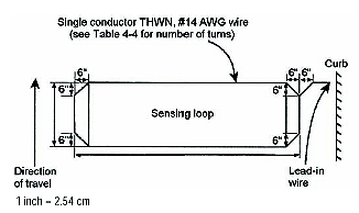
Figure 4-14. Wide inductive-loop detector layout.
Number of lanes |
Total approach width of lanes |
Loop width |
Loop length |
Turns of wire |
|||
|---|---|---|---|---|---|---|---|
feet |
meters |
feet |
meters |
feet |
meters |
||
1 |
12–18 |
3.7–5.6 |
6–12 |
1.8–3.7 |
6 |
1.8 |
4 |
2 |
19–32 |
5.7–9.8 |
13–26 |
3.7–8.1 |
6 |
1.8 |
3 |
3 |
33–45 |
9.9–13.6 |
27–39 |
8.2–12.1 |
6 |
1.8 |
2 |
4 |
46–52 |
13.7–15.8 |
40–46 |
12.2–13.7 |
6 |
1.8 |
1 |
Large loops of up to 30 ft (9 m) in width and 50 to 60 ft (15 to 18 m) in length have been installed to extend green time when occupancy increases to a saturation level in a given direction. The inductive-loop detector electronics unit is adjusted to be sensitive to more than some specified number of vehicles in the loop. Thus, the electronics unit only responds to a saturated condition. No additional green extension is given to the approach unless there is congestion. If no extensions are present (i.e., there is no saturation or congestion), the opposing street green receives the excess time. This application cannot be used for call initiation and is intended for use only in locations where unpredictable and extreme fluctuations of traffic are present, such as shopping center exits, some freeway exits onto main street flow, and industrial plant parking lot exits.
Vehicle sensors in left-turn lanes can affect the capacity of an intersection by reducing unnecessary green time and left turn arrow indications. When the last vehicle proceeds a block or so past the signal before the conflicting phase begins, the travel time represents lost green time, which could more appropriately be used to increase the green time available to other phases. The design of left-turn detection is generally based on the premises discussed below.
From 3 to 5 seconds are normally required at the start of the green indication for the first vehicle in a queue to start up, with an average headway of 2 to 3 seconds between following vehicles. Longer startup and headway times are accounted for by providing an appropriate loop length to maintain the green for these slower vehicles. Moreover, trucks and other slow vehicles may require a still longer startup time, which frequently results in a three or four car-length gap ahead of them. Loop length also needs to account for these gaps.
Because green time is based on vehicular demand, only a short green time is needed for one or two vehicles. For example, a rapidly starting single vehicle can clear the turn lane with a green time of less than 5 seconds. A driver of a following vehicle just entering the left turn lane may be confused by the short green. The length of the inductive loop should allow the following car to reach the loop in time to enter the intersection on the green indication or brake to a stop. This length is based on the equation for maximum deceleration rates, which indicates that a vehicle traveling at 30 mi/h (48 km/h) can stop in 83 ft (25 m).
To accommodate these conditions, a loop length of 80 ft (24 m) from the stopline and a controller passage time of 1 second are frequently used. Adding more passage time on the controller compensates for passage over shorter loops. Controller passage time is the time a controller holds the green after actuation. A passage time of 1.0 second permits most motorists to almost complete their turning radius before the onset of the yellow change interval is displayed.
Another problem occurs when vehicles are permitted to turn on the circular green (green ball) indication. Drivers will usually proceed past the stopline and wait for a gap in the opposing traffic. If a gap does not occur or a vehicle ahead prevents the turn, the driver may be left stranded beyond a detection zone that ends at the stopline. In this case, the controller may skip the turn arrow in the next cycle because the vehicle is positioned ahead of the sensor's detection zone. Some agencies think it a good practice to extend the loop beyond the stopline 1 to 6 ft (0.3 to 2 m) to prevent this situation.
Small-vehicle (e.g., motorcycle) detection using short inductive loops requires a high sensitivity setting on the electronics unit. However, high sensitivity will frequently cause detection of vehicles in adjacent lanes (splashover). Many agencies use quadrupole loops to avoid splashover. As the quadrupole requires an additional sawcut equal to the length of the loop, it is desirable to limit quadrupole installation to the area near the stopline. Quadrupole design is discussed further under the topic of "Detection of Small Vehicles."
Figure 4-15 illustrates a minimum-length quadrupole left-turn loop designed by the Illinois DOT (IDOT) using the procedure below:(6)
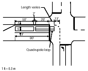
Figure 4-15. Left turn detection inductive-loop configuration used by IDOT.
When the left-turn demand requires 150 ft (45 m) or more of storage length or when higher approach speed requires long deceleration lanes, the loop layout should include an advanced detection loop. The advanced vehicle sensor with a call extension feature will extend the effective detection zone to accommodate heavy traffic volumes or high-speed traffic.
Detection of vehicles in through lanes depends on the approach speed and the type of controller operation being used. Single-point detection, long-loop occupancy detection, a combination of long and short loops, or a sequence of short loops can be deployed. Each of these is discussed below.
This is the simplest type of vehicle detection used for actuated controllers. It is primarily found on low-speed approaches where speeds are less than 35 mi/h (56 km/h). It may also be used on side-street approaches, with another form of detection on the major street.
A point vehicle sensor (e.g., a 6- x 6-ft (1.8- x 1.8-m) inductive loop) is located 2 to 4 seconds of travel time in advance of the stopline. As this is the only sensor in the approach lane, controller timing must be appropriately set to use the information. The actual distance divided by 25 ft (7.6 m) (which approximates the length of a vehicle plus the space between vehicles) indicates the number of vehicles that can be queued between an inductive-loop detector and the stopline when the light turns green. This number establishes the minimum green interval for the controller. The distance between the inductive loop and the stopline divided by the 15th percentile speed provides a good initial estimate of the passage time. The passage time is also the allowable gap that causes the green indication to drop. If this setting is too long or short to be acceptable as an allowable gap, the position of the loop should be moved to ensure an appropriate gap size.
Loop-occupancy detection is generally used on low-speed approaches. It normally consists of a single loop 50 ft (15 m) or more in length or a sequence of short loops (usually four) located immediately upstream of the stopline. Loop-occupancy timing is used on the controller as described earlier. This type of operation is most effective when speeds are 25 mi/h (40 km/h) or less. Even at this speed, there is some potential for the signal turning yellow just before an approaching vehicle reaches the loop. In this case, the vehicle will probably cross the intersection on the yellow indication.
As speeds increase, the detection zone must lengthen to accommodate the increased stopping distance. One jurisdiction uses the combination of approach speeds and loop lengths shown in Table 4-5. These loop lengths appear to be excessively long, resulting in long minimum gaps.
The 120-ft (37-m) detection area is measured from the stopline and consists of two 56-ft (17-m) loops. Where greater detection areas are required, either additional long loops or small loops may be used. If additional small loops are chosen, they must be connected to separate electronics units with the extension time programmed into the unit. The long loops are set to presence mode.
Speed |
Loop length |
||
|---|---|---|---|
mi/h |
km/h |
feet |
meters |
30 |
48 |
120 |
37 |
35 |
56 |
160 |
49 |
40 |
64 |
200 |
61 |
45 |
72 |
250 |
76 |
For high-speed approaches (those with speeds greater than 48 km/h (30 mi/h)), detection becomes more complex. Volume-density control is one technique used that relies on the controller functions rather than extensive detectorization. Normally only one sensor is installed in each lane. This point sensor is usually placed at least 5 seconds and as much as 8 to 10 seconds from the stopline, which is more than the 2 to 4 seconds of travel time required for normal actuated operation.
The sensor is active at all times rather than just during the green interval. During the red interval, each actuation increments the variable initial timing period. Once the variable initial timing period exceeds the minimum green, each additional actuation adds an additional user specified time increment to the initial interval. If the variable initial timing does not exceed the initial interval, then that duration is used instead for the first portion of the green interval. During the green interval, the sensor is used to extend the green. At first the extension is equal to the passage time, but after a conflicting phase has registered a call, the extension is reduced, eventually reaching a minimum gap.
This type of signal control has the potential for trapping a vehicle in the dilemma zone at the onset of yellow. The following section discusses dilemma zones and describes how multiple sensors are used to alleviate the dilemma zone problem.
Signalized intersections where speeds of approaching traffic are greater than 30 mi/h (48 km/h) have long been of concern to designers and operations and safety engineers. Drivers approaching at these higher speeds are frequently confronted with a dilemma—whether to stop or proceed through the intersection at the onset of the yellow change interval. The placement of sensors to ameliorate this problem has received serious consideration and research. This section defines the many variables that affect the dilemma zone problem and describes several sensor placement schemes that have proven effective.
When a vehicle traveling at a constant speed S approaches an intersection and is positioned at distance X from the intersection at the beginning of the yellow change interval, the driver is faced with a decision. He may decelerate and stop the vehicle before entering the intersection or continue and enter the intersection, accelerating if necessary before the red interval begins. In some States, the driver is required to clear the intersection before the red appears. Depending on the distance from the intersection and the speed of travel, drivers may not be certain that they can stop in time, or they may be unsure that they can clear the intersection before conflicting vehicles enter. This creates the dilemma. Some drivers will opt to stop, while others may accelerate and continue through the intersection.
If the choice is to stop, the driver will decelerate after a short perception and reaction time. The distance the vehicle travels after the beginning of the yellow change indication includes the distance traveled during the perception and reaction time t and the distance traveled during deceleration. The inequality that must be maintained to ensure a safe and complete stop is given by
 (4-2)
(4-2)
where
X = distance from stopline at start of yellow interval, ft (m)
S = approach speed, ft/s (feet per second) (m/s (meter per second)
t = perception and reaction time (typically, 1 second)
d = constant deceleration rate, ft/s2 (m/s2).
Safety and comfort require that the vehicle's deceleration rate not exceed one-third to one-half the acceleration of gravity. Using d* to represent a critical deceleration rate under prevailing roadway conditions, a stopping distance Xs may be defined as
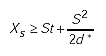 (4-3)
(4-3)
where Xs is the minimum distance from the stopline in which the vehicle can come to a complete stop after the beginning of the yellow interval. Thus, if a vehicle is closer to the stopline than Xs when the yellow begins, the driver will be unable to stop safely or comfortably before the intersection. The area between the stopline and Xs is an area in which drivers should not be expected to stop or cannot stop as shown in the upper portion of Figure 4-16.
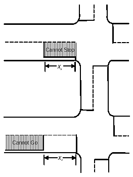
Figure 4-16. "Cannot Stop" and "Cannot Go" regions.
If the driver decides to accelerate and pass through the intersection, a clearance distance Xc must be maintained as defined by the inequality:
Equation 4-4 is based on the general relationship that distance traveled Xc = X0 + St + 0.5at2, where X0 is some initial distance. |
![]() (4-4)
(4-4)
where
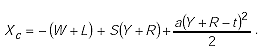
Xc = clearance distance, ft (m)
t = perception and reaction time (typically 1 second)
a = acceleration rate, ft/s2 (m/s2)
Y = yellow change interval, seconds
R = red clearance interval, seconds
W = effective width of intersection, ft (m)
L = length of vehicle, ft (m)
S = approach speed, ft/s (m/s)
W + L = correction to stopbar distance to bring the rear of the car beyond the intersection.
Implementing Equation 4-4 permits the driver to completely clear the intersection before the appearance of the red signal. Many traffic engineers do not believe that a driver must clear the intersection on the yellow. In fact, most State vehicle codes do not require the vehicle to clear the intersection prior to the onset of the red indication, but merely to have entered prior to the red. If this interpretation applies, engineers may eliminate the (W + L) term from the equation or may use 0.5 or 0.25 of the value of this term. In some cases, the red clearance interval is increased to assure clearance when needed rather than include the (W + L) term in the equation.
The constant acceleration rate a available to the driver in Equation 4-4 may be estimated from Gazi's equation as
![]() (4-5a)
(4-5a)
or
![]() (4-5b)
(4-5b)
These equations show that larger acceleration rates can be attained when a vehicle is traveling at lower speeds. Clearance distance Xc is the maximum distance from the stopline at which a vehicle can clear the intersection as defined by
 (4-6)
(4-6)
Since Xc is the maximum distance upstream of the stopline from which a vehicle can clear the intersection during the yellow interval, any vehicle positioned at a point beyond Xc (i.e., further upstream) would not be expected to clear the intersection during the yellow interval, and is thus in a region in which the driver "cannot go" without violating the red indication (see lower portion of Figure 4-16).
As both Xs and Xc are measured distances from the stopline, the relationship of these two quantities is defined by one of the following conditions:
When Xs > Xc, the dilemma zone is the overlapping area in which a vehicle can neither stop nor go if faced with a yellow indication as indicated in Figure 4-17. In this case, the driver of a vehicle within the dilemma zone at the onset of yellow has to accelerate or decelerate at an unsafe rate and consequently is vulnerable to a right-angle or rear-end accident.
When Xs = Xc, Figure 4-18 shows that the dilemma zone and its associated problems disappear. A driver in the "cannot go" region is able to stop safely, whereas a driver in the "cannot stop" region can successfully accelerate through the intersection.
Finally, when Xs < Xc, a driver in the area between Xs and Xc may either stop or go safely. Therefore, this region is considered an optional zone as depicted in Figure 4-19.
This relatively simply analysis indicates that a dilemma zone is only formed when Xs > Xc. Equation 4-3 shows that Xs is a function of speed, perception and reaction time, and deceleration rate, while Equation 4-4 shows that Xc is a function of speed, perception and reaction time, acceleration rate, yellow and red interval times, and effective width of the intersection.
Tables 4-6 (English units) and 4-7 (metric units) contain stopping distance Xs and clearance distance Xc for deceleration rates of 10 and 16 ft/s2 (3.0 and 4.9 m/s2) for an intersection width of 48 ft (15 m). Tables 4-8 (English units) and 4-9 (metric units) repeat the stopping and clearance distances for the same deceleration rates for an intersection width of 76 ft (23 m).
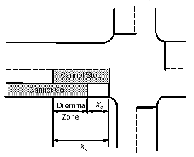
Figure 4-17. Dilemma zone (Xs > Xc).
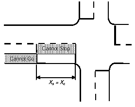
Figure 4-18. Dilemma zone removal (Xs = Xc).
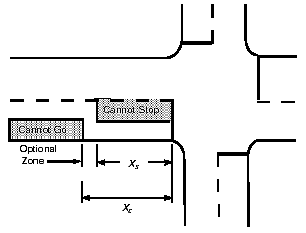
Figure 4-19. Optional zone creation (Xs < Xc).
Tables 4-16 through 4-19 are based on the following assumptions:
Several general conclusions from the analysis of the dilemma zone problem are:
Decel. rate |
Speed |
Stopping distance |
Clearance distance (ft) for yellow interval equal to: |
||
|---|---|---|---|---|---|
ft/sec2 |
mi/h |
feet |
3 sec |
4 sec |
5 sec |
| 10 | 20 |
73 |
39.5 |
93.2 |
156.6 |
25 |
104 |
58.3 |
115.5 |
180.8 |
|
30 |
141 |
77.2 |
137.8 |
205.0 |
|
35 |
184 |
96.1 |
160.1 |
229.1 |
|
40 |
232 |
115.0 |
182.4 |
253.3 |
|
45 |
285 |
133.8 |
204.7 |
277.5 |
|
50 |
344 |
152.7 |
227.0 |
301.7 |
|
55 |
408 |
174.0 |
254.6 |
335.3 |
|
60 |
477 |
196.0 |
284.0 |
372.0 |
|
16 |
20 |
56 |
39.5 |
93.2 |
156.6 |
25 |
79 |
58.3 |
115.5 |
180.8 |
|
30 |
105 |
77.2 |
137.8 |
205.0 |
|
35 |
134 |
96.1 |
160.1 |
229.1 |
|
40 |
167 |
115.0 |
182.4 |
253.3 |
|
45 |
203 |
133.8 |
204.7 |
277.5 |
|
50 |
242 |
152.7 |
227.0 |
301.7 |
|
55 |
285 |
174.0 |
254.6 |
335.3 |
|
60 |
331 |
196.0 |
284.0 |
372.0 | |
Decel. rate |
Speed |
Stopping distance |
Clearance distance (m) for yellow interval equal to: |
||
|---|---|---|---|---|---|
m/sec2 |
km/h |
meters |
3 sec |
4 sec |
5 sec |
| 3 | 20 |
73 |
10.3 |
26.4 |
45.7 |
25 |
104 |
13.8 |
30.6 |
50.2 |
|
30 |
141 |
17.4 |
34.8 |
54.8 |
|
35 |
184 |
24.6 |
43.3 |
64.0 |
|
40 |
232 |
31.7 |
51.7 |
73.1 |
|
45 |
285 |
38.9 |
60.2 |
82.3 |
|
50 |
344 |
42.4 |
64.4 |
86.9 |
|
55 |
408 |
46.0 |
68.6 |
91.4 |
|
60 |
477 |
54.0 |
79.0 |
104.0 |
|
| 5 | 20 |
56 |
10.3 |
26.4 |
45.7 |
25 |
79 |
13.8 |
30.6 |
50.2 |
|
30 |
105 |
17.4 |
34.8 |
54.8 |
|
35 |
134 |
24.6 |
43.3 |
64.0 |
|
40 |
167 |
31.7 |
51.7 |
73.1 |
|
45 |
203 |
38.9 |
60.2 |
82.3 |
|
50 |
242 |
42.4 |
64.4 |
86.9 |
|
55 |
285 |
46.0 |
68.6 |
91.4 |
|
60 |
331 |
54.0 |
79.0 |
104.0 | |
Decel. rate |
Speed |
Stopping distance |
Clearance distance (ft) for yellow interval equal to: |
||
|---|---|---|---|---|---|
ft/sec2 |
mi/h |
feet |
3 sec |
4 sec |
5 sec |
| 10 | 20 |
73 |
11.5 |
65.2 |
128.7 |
25 |
104 |
30.4 |
87.5 |
152.9 |
|
30 |
141 |
49.3 |
109.8 |
177.0 |
|
35 |
184 |
68.1 |
132.1 |
201.2 |
|
40 |
232 |
87.0 |
154.4 |
225.4 |
|
45 |
285 |
105.9 |
176.7 |
249.5 |
|
50 |
344 |
124.8 |
199.0 |
273.7 |
|
55 |
408 |
146.0 |
226.7 |
307.3 |
|
60 |
477 |
168.0 |
256.0 |
344.0 |
|
| 16 | 20 |
56 |
11.5 |
65.2 |
128.7 |
25 |
79 |
30.4 |
87.5 |
152.9 |
|
30 |
105 |
49.3 |
109.8 |
177.0 |
|
35 |
134 |
68.1 |
132.1 |
201.2 |
|
40 |
167 |
87.0 |
154.4 |
225.4 |
|
45 |
203 |
105.9 |
176.7 |
249.5 |
|
50 |
242 |
124.8 |
199.0 |
273.7 |
|
55 |
285 |
146.0 |
226.7 |
307.3 |
|
60 |
331 |
168.0 |
256.0 |
344.0 | |
Decel. rate |
Speed |
Stopping distance |
Clearance distance (m) for yellow interval equal to: |
||
|---|---|---|---|---|---|
m/sec2 |
km/h |
Meters |
3 sec |
4 sec |
5 sec |
| 3 | 30 |
19.9 |
2.3 |
18.4 |
37.7 |
35 |
25.5 |
5.8 |
22.6 |
42.2 |
|
40 |
31.7 |
9.4 |
26.8 |
46.8 |
|
50 |
46.0 |
16.6 |
35.3 |
56.0 |
|
60 |
63.0 |
23.7 |
43.7 |
65.1 |
|
70 |
82.5 |
30.9 |
52.2 |
74.3 |
|
75 |
93.2 |
34.4 |
56.4 |
78.9 |
|
80 |
104.5 |
38.0 |
60.6 |
83.4 |
|
90 |
129.2 |
46.0 |
71.0 |
96.0 |
|
| 5 | 30 |
15.3 |
2.3 |
18.4 |
37.7 |
35 |
19.2 |
5.8 |
22.6 |
42.2 |
|
40 |
23.5 |
9.4 |
26.8 |
46.8 |
|
50 |
33.2 |
16.6 |
35.3 |
56.0 |
|
60 |
44.4 |
23.7 |
43.7 |
65.1 |
|
70 |
57.3 |
30.9 |
52.2 |
74.3 |
|
75 |
64.2 |
34.4 |
56.4 |
78.9 |
|
80 |
71.6 |
38.0 |
60.6 |
83.4 |
|
90 |
87.5 |
46.0 |
71.0 |
96.0 | |
In pretimed signal control, the appropriate strategies for controlling the dilemma zone problem consist of providing a consistent yellow change interval and incorporating an appropriate red clearance interval. This strategy will, however, increase vehicular delay.
In actuated signal controlled intersections, the most appropriate strategy for resolving the dilemma zone problem involves sensor placement before, within, and after the dilemma zone in such a way as to reduce the probability of entrapment of a vehicle in the dilemma zone at the onset of the yellow interval. The various methods of sensor placement for dilemma zones are discussed below.
The dilemma zone problem can be ameliorated by the strategic placement of multiple sensors at high-speed approaches to intersections controlled by actuated controllers. The mitigation methods described below assume the use of inductive-loop detector systems operating in the presence mode. As inventive as the procedures are, vehicles will still get caught in the dilemma zone because of maximum greens, force-offs, etc. Consequently, adequate change intervals (yellow and all-red displays) must be provided to ensure motorist safety.
The three sensor placement strategies in general use for multiple-point detection are:
A green extension system consists of an assembly of extended call sensors and auxiliary logic, which enable vehicles to be detected before entering the dilemma zone and provide the controller with data to extend the green until the vehicles clear the dilemma zone.(9) The logic monitors the signal display, enables or disables selected call sensors, and holds the controller in green. Although two loops are normally employed, three may be used at high-speed intersections. Figure 4-20 shows loop placement for vehicles traveling at the 85th percentile speed.(10)
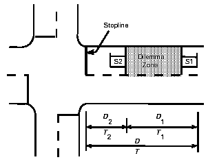
Figure 4-20. Green extension system using two inductive-loop detectors.
The appropriate distances for placing the loops are calculated using
 (4-7)
(4-7)
 (4-8)
(4-8)
![]() (4-9)
(4-9)
where
S = 85th percentile speed, mi/h (km/h)
t = perception and reaction time, seconds
f = coefficient of friction
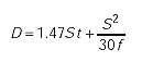
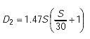
D = stopping distance, ft (m)
D2 = clearing distance, ft (m)
D1 = separation between loops, ft (m).
With the loops positioned as shown, a vehicle passing over loop S1 actuates an electronic timer, which extends the green for the vehicle to reach loop S2 in time T1. Similarly, when the vehicle passes over loop S2, a second timer maintains the green while the vehicle proceeds toward the intersection. This design does not insure that vehicles traveling at speeds less than the 85th percentile speed would not be trapped in the dilemma zone.
This concept uses a 70-ft (21-m) presence loop extending upstream from the stopline and a small extended call loop 250 to 500 ft (75 to 150 m) upstream of the stopline, as shown in Figure 4-21. The magnitude of D is calculated from Equation 4-7, using the speed limit or the 85th percentile speed. D2 is set equal to 70 ft (21 m). Time T1 is calculated as D1 (found from Equation 4-9) divided by a lower-limit approach speed, which is generally assumed equal to the 15th percentile speed. This time is programmed into the extended-call electronics unit. The controller is operated in the loop occupancy control mode.
Proper design of an extended-call detection system ensures that the last vehicle and those vehicles traveling below the speed limit are not trapped in the dilemma zone. A trailing vehicle may be trapped at the end of the maximum-extension limit (maximum green time after an actuation on an opposing phase). The 70-ft (21-m) presence loop guarantees that stopped vehicles queued behind the stopline will move forward and enter the intersection without triggering a premature gap out.
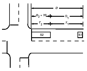
Figure 4-21. Extended call inductive-loop detector system.
The green extension and the extended-call detection systems used two or (at most) three sensors. These techniques can be used effectively at intersections with relatively low speeds. However, when speeds are high, the dilemma zone becomes longer, and more sensors are needed to accommodate the large range of approach speeds that are generated. Three techniques are commonly used for determining the placement of the required sensors. These methods are identified by the developer, agency, or organization that pioneered the technique.
Beierle Method: This method (originated by Harvey Beierle of the Texas DOT(11) (TxDOT) uses a 1-second vehicle interval setting on a controller operating with locking detection memory. The sensors are 6- x 6-ft (1.8- x 1.8-m) presence mode inductive loops.
The outermost sensor upstream of the intersection is placed at a safe stopping distance from the intersection for highest normal approach speed. Safe stopping distances are based on a 1-second perception and reaction time plus braking distances resulting from coefficients of friction between 0.41 and 0.54 for speeds between 55 and 20 mi/h (90 and 30 km/h). The next sensor is tentatively located at a safe stopping distance for a vehicle traveling 10 mi/h (16 km/h) less than that assumed for the first sensor. If the travel time between the two sensors is greater than 1 second, the downstream sensor is relocated to allow the vehicle to reach the second sensor within the 1-second vehicle interval set on the controller.
This location procedure is repeated for each successive sensor until the last loop is within 75 ft (23 m) of the stopline, each time subtracting 10 mi/h (16 km/h) from the maximum considered speed. The minimum assured green time is set on the controller to permit vehicles stopped between the last sensor and the intersection to enter the intersection.
TxDOT examined a modification to the Beierle procedure, which uses American Association of State Highway and Transportation Officials (AASHTO) stopping distance criteria. Figure 4-22 illustrates the sensor spacing for speeds common to Texas.
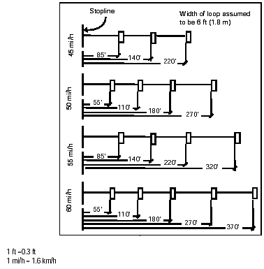
Figure 4-22. Multiple inductive-loop detector placement (TxDOT) for alleviating the effects of dilemma zones.
Winston-Salem Method: The second method of multiple sensor placement was developed by Donald Holloman for that agency.(9) It is basically the same as the Beierle Method. The Winston-Salem Method differs by using a slightly shorter stopping distance for the outermost and innermost sensor and incorporates speeds up to 60 mi/h (97 km/h).
SSITE Method: The third method was developed by the Southern Section of the Institute of Transportation Engineers (SSITE).(12,13) It uses an iterative process and engineering judgment in locating the sensors. The outermost loop is positioned to provide safe stopping distance, as determined by data collected by the Southern Section. The differences with respect to the other multiple sensor methods are:
Tables 4-10 and 4-11 summarize the characteristics of the extended call and multiple point detection methods with respect to the number of loops and their spacing. Since the length of the dilemma zone becomes larger as speed increases, more sensors are required to track the vehicle through the dilemma zone. Moreover, larger spacing between sensors implies detection of only larger vehicle intervals and less efficient controller operation.
In general, it appears that the multiple point detection methods are more appropriate for use with high mean approach speed and high flow variability.
Green extension systems for the semiactuated controllers method |
Extended-call detection systems for basic controllers method |
|
|---|---|---|
Parameter |
Value |
Value |
Controller memory |
Nonlocking |
Nonlocking |
Sensor type |
Presence |
Presence |
Speed range |
S = 85th percentile |
S = 85th percentile |
Outermost loopa |
|
|
Innermost loop |
|
0 |
Spacing between loopsb |
|
|
Number of Loops |
2 (or 3) |
2 |
Allowable gap |
5 to 6 Seconds |
5 to 6 Seconds |
a. Distance D is measured from the stopline.
b. Slow limit = Low speed limit; for example, 15th percentile speed.
Beierle Method |
Winston-Salem Method |
SSITE Method |
|
|---|---|---|---|
Controller memory |
Locking |
Nonlocking |
Nonlocking |
Sensor type |
Presence |
Presence |
Presence |
Speed range |
S ≤ 50 |
S ≤ 60 |
S ≤ 60 |
Outermost loopa |
Use stopping distance from Beierle, Ref. 11 |
Use stopping distance from Sackman, Ref. 9 |
Use Southern Section ITE Report, Ref. 12 |
Innermost loop |
Within 75 ft (23 m) of approach stopline |
86 ft (26 m) |
00 |
Spacing between loopsb |
1 second |
1 second |
2 seconds |
Number of Loops |
|
|
≤ 6 |
Allowable gap |
2 to 5 seconds |
2 to 5 seconds |
5 to 7 seconds |
a. Distance D is measured from the stopline.
b. Slow limit = Low speed limit; for example, use 15th percentile speed.
c. ![]() represents the integer part of S/10; for example
represents the integer part of S/10; for example ![]()
To simplify their sensor design process, PennDOT defined seven basic design options together with an evaluation of the characteristics of each option. The following excerpt describes these options from the PennDOT Traffic Signal Design Handbook.(14)
Option 1: Consists of a long loop 6 x 50 ft (1.8 x 15 m) maximum for each approach lane. This enables individual lane detection in the presence mode. Although it requires more loop wire than the other options, its initial cost is the lowest as less lead wire and fewer pull boxes are required. Construction cost is lowest of all options. The disadvantages include: all detection for a lane is lost should the loop break and long loops are the least sensitive of all loop configurations. When the sensitivity is increased, the loop becomes more susceptible to detecting vehicles in adjacent lanes.
Option 2: Consists of sequential short loops for individual lane detection in either the pulse or presence mode. They may be wired either in series or parallel; however, best results are achieved when alternate loops are paired and wired in parallel to separate input channels. There is an added safety feature inherent to this option in that should one loop fail, detection is not completely lost. Although the initial cost is higher than that for long loops, maintenance is easier, as only a small loop need be replaced in case of damage.
Like the long loop, the short loops are susceptible to detecting vehicles in adjacent lanes; however, they are more sensitive and are better suited for sensing small vehicles.
Option 3: Consists of a long quadrupole loop for each approach lane. Its operation is identical to that of Option 1. The major advantages of Option 3 are increased sensitivity for detecting bicycles and small motorcycles, coupled with its ability to reject detection of vehicles in adjacent lanes. Like Option 1, detection for an entire lane is lost if the loop be severed. Construction cost is approximately 20 percent greater than for Option 1.
Option 4: Consists of one short loop per lane located in advance of the intersection based on normal approach speeds. This option, which operates in pulse mode only, is best suited for providing extension intervals on roads with higher travel speeds.
The loops installed for Option 4 can also be used for individual lane counting and gap determination. There are two disadvantages with this option. First, should the loop fail, detectorization for the approach is lost. Second, since there are no loops near the stopline, any vehicle entering the approach from a driveway between the loop and the stopline is not detected and has to wait for another vehicle to place a call for the necessary phase unless calling detectors are installed.
Option 5: Basically the same as Option 4, except a single wide loop is used for multilane detection instead of individual lane sensors. Construction is less expensive than Option 4; however, should breakage occur, detection on that approach is completely lost.
Option 6: Consists of a single short loop per approach lane for use where a driveway is located between the intersection and the area of detection for Options 4 or 5. Traffic generated by the driveway is unable to actuate its phase without the additional loops placed near the stopline. A 6-ft x 6-ft (1.8-m x 1.8-m) calling inductive loop is used in these cases.
Several applications require inductive-loop detector systems to perform unique functions. These include small-vehicle and bicycle detection, detection of long vehicles or large trucks, queue detection at freeway off-ramps, vehicle counting, and special safety applications to prevent accidents and reduce speeds.
Summaries of various loop shapes and operating characteristics are given below in terms of the functional requirements determined by the operating agency. These requirements are typically based on the type of application (e.g., intersection control and freeway surveillance and control), traffic or vehicle mix, climate, and other site-specific conditions.
Increased fuel costs tend to accelerate the proclivity for smaller, fuel-conserving vehicles. These range from small compact automobiles to l00-cc motorcycles, mopeds, and lightweight bicycles. The increasing number of these small vehicles and their behavior patterns often necessitates their detection with existing standard inductive-loop detector configurations.
A presence sensor should be able to detect a small motorcycle and hold its call until the display of a green signal. If the sensor drops a call prematurely, the motorcyclist could be trapped on the red phase. The required hold time should at least match the shortest cycle time observed at the intersection. The NEMA Standards (see appendix J) specify a minimum hold period of 3 minutes.
Calls may be dropped prematurely in some older inductive-loop electronics units that include the ability to compensate for environmental drift, primarily due to changes in temperature and moisture. This circuitry will frequently neutralize a weak detection from a small vehicle within a period of less than a minute. Newer electronics units do not have this problem and all meet the NEMA Standards and the Type 170 Specification, which both require a minimum hold time of 3 minutes.
In California and other temperate areas, the bicycle has become a common mode of transportation. As such, properly signalized intersection operation and safety require detection of bicycles. The inherent problems associated with bicycle detection include:
In response to these problems, it has been suggested that the inductive- loop electronics unit have extension timing and delay features. In such a system, one loop is located about 100 ft (30 m) from the stopline, and the second loop is located at the stopline. When a bicycle is detected at the first loop, the extension time is provided to hold the green to allow the bicycle to reach the loop at the stopline.
When the detection is made at the stopline, extension time is provided to allow the bicycle to move far enough into the intersection to safely clear before the end of the yellow indication. If the detection occurs when the light is red, the minimum timing feature assures that when the light turns green, the minimum green time will allow safe crossing of the intersection. This type of operation works best in a bike lane. The loop in the bike lane with a standard electronics unit could be wired to call the pedestrian timing, which would allow adequate time for the cyclist to cross the intersection.
A delay feature is used where vehicles merge into the bike lane to turn right. The detection is not immediately registered so that the vehicle may complete a right turn without creating delay for other traffic including bicycles.
A number of factors determine the most effective inductive-loop configuration needed to satisfy policies that dictate detection of small vehicles, including bicycles. Important criteria include shape of the loop, width of the lane, and loop placement within that lane. Loop configurations that enhance the ability to detect small vehicles are described below.
A configuration frequently used for the detection of small vehicles is multiple, interconnected small loops or, as it is often referred to, sequential short loops. The sensitivity can be better controlled with the multiple loops than with the conventional single long loop, whose sensitivity must be set so high for small-vehicle detection that false calls from adjacent lanes (splashover) result. With the small loops, total-loop inductance very close to optimum can be achieved by connecting the loops in series. In the past, series/parallel connections were mandated; however, newer electronics units have obviated this need. Moreover, the small vehicle will be detected when it reaches the first small loop rather than at the stopline, as is the case with the long loop with a powerhead described later. Also, should one loop fail, some detection capability still remains in that lane.
The quadrupole-loop configuration was first used in the early 1970s. As shown in Figure 4-23, this configuration adds a longitudinal sawcut in the center of the lane. The loops are wired in a figure-eight pattern so that the center wires have current flowing in the same direction. Their fields reinforce each other, improving the capability to detect small vehicles. The center wires counteract the fields of the outer wires, which have their current flowing in the opposite direction from the center wires. The influence of the outer fields is diminished, thereby reducing the possibility of splashover.
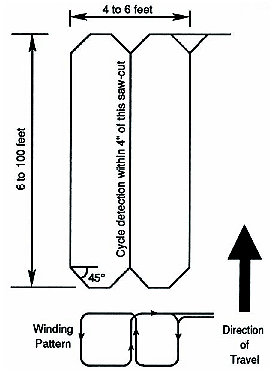
Figure 4-23. Quadrupole loop configuration.
The single-wire configuration ("1-2-1" with one layer in the perimeter slots and two layers in the center slot), shown in Figure 4-23, is used for the detection of automobiles, trucks, and the larger motorcycles. A double layer design ("2-4-2") is recommended for detecting small motorcycles and bicycles. Some agencies wind the 2-4-2 as two, 2-turn loops rather than the traditional, figure-eight winding pattern. No definitive tests were found to favor either method.
Loop placement in the lane is another important consideration. Installation in the center of the lane may fail to detect the small motorcycle if the travel path is outside the quadrupole field. For example, motorcyclists waiting to turn left will usually stop on the left side of the lane and thus may be outside of the quadrupole field. Where detection is required for a left-turn lane, it is recommended that the left edge of the quadrupole be located no further than 2 ft (61 cm) from the left edge of the left-turn lane.
The quadrupole is used as a short or long loop, a single element, and in combinations such as series or series/parallel. The series/parallel configuration is used effectively across the country not only to detect small vehicles, but also to eliminate the problem of adjacent-lane detection (splashover) in high-sensitivity inductive-loop systems.
Short quadrupoles (those less than 30 ft (9 m)) tend to lose high-bed sections of trucks. Since the quadrupole is really two loops whose field detection height is approximately two-thirds of the short leg of the loop, the approximate detection height is 2 ft (0.6 m). This detection height is based on the dimension of two 3-ft- (0.9-m-) wide side-by-side quadrupole loops. With longer loops (those greater than 30 ft (9 m)), there are always one or more wheels or axles over the loop.
It is generally agreed that the 6-ft (1.8-m) quadrupole loop detects bicycles better than most other loop configurations. The major problem with this configuration for small-bicycle detection is the need for the bicyclists to ride close enough to a wire within the quadrupole to be detected. A number of unique pavement markings and signs have been developed to assist this application. The pavement marking identifies the location of the wire and the sign explains the markings to the cyclist.
Figure 4-24 illustrates a marking system used in Clarke County, GA. A pattern of 4- x 18-inch (10- x 46-cm) white stripes is placed 18 inches (46 cm) apart, starting at the stopline. The length is kept short since only one actuation is necessary to call the green indication.
In the City of San Luis Obispo, CA, an aggressive public information program was mounted to inform bicyclists that they could cause the red light to turn green by traveling over the bicycle-shaped pavement marking shown in Figure 4-25. These markings were painted on all appropriate through, right-, and left-turn lanes at all signalized intersections that contained loop sensors.
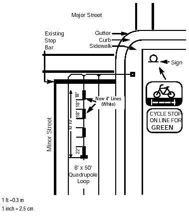
Figure 4-24. Bicycle sensor sign and markings used in Clarke County, GA.
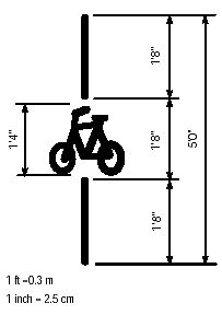
Figure 4-25. Special bicycle pavement marking used in San Luis Obispo, CA.
Small vehicles can be detected with the chevron configuration shown in Figure 4-26. It consists of one or more four-turn parallelogram loop(s) with the short section in the direction of traffic and the long section at an angle of 30° with the short section. The long sides of the loop sections are 27.5 inches (70 cm) apart. Adjacent ends of successive loop sections may be in a single slot or separated by 2 ft (61 cm). This alignment allows a vehicle to cut the lines of flux more efficiently.(15)
Loop sections are wound alternately clockwise and counterclockwise so that currents in adjacent loop ends are always in the same direction. Successive sections wound in the same direction would produce dead paths where the sections are joined.
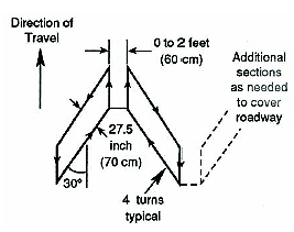
Figure 4-26. Chevron-loop configuration.
Frequently, a small motorcycle or bicycle will not produce a sufficient shift of inductance in a one-turn 6 x 20 ft (1.8 x 6.1 m) or longer loop. Some inductive-loop electronics units will detect these small vehicles with two or more turns of wire although there are dead areas in the center of the loop.
One approach is to use a small powerhead at the stopline with the long loop. This configuration is shown in the upper portion of Figure 4-27. The standard powerhead can be improved by angling the transverse wires as shown in the lower portion of Figure 4-27. The angling will cause the small vehicle to cut the lines of flux more efficiently, thereby increasing the signal by as much as 25 percent. The disadvantage is that the vehicle may not stop on the powerhead unless the detection area is clearly indicated by paint or signs.
Some traffic engineers have concerns about liability because small vehicles are not detected throughout the detection zone. Although these vehicles are sensed at the stopline, the controller operation is based on the detection of vehicles in the approach. Other engineers feel that the important consideration is to detect the small vehicles to ensure they receive the green signal, not to ensure that the signal operation is optimized for these vehicles. They do not believe that any liability is incurred.
Use of sequential short loops rather than a single long loop avoids nondetection of small vehicles anywhere in the detection zone. Also, modern electronics units sense small vehicles without the resultant splashover that occurs when using the single long loop with high-sensitivity settings. These two factors have reduced the need for the powerhead design.
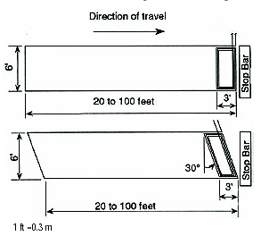
Figure 4-27. Long loop with powerhead.
Caltrans developed a Type D loop configuration to better detect bicycles.(16) This configuration, shown in Figure 4-28, is a palm-shaped loop that fits into a 6-ft (1.8-m) square. The loop has three turns of wire when a single Type D loop is connected to an electronics unit channel, and five turns if one Type D loop is connected in series with three 6- x 6-ft (1.8- x 1.8-m) loops on an electronics unit channel (see Type 5DA or 5DQ installations in Figure 4-12). This configuration requires that the wire be protected where it bends around the acute corners of the cut. Drilling a hole in the corner or chipping out the inner angle to provide a radius will prevent kinking of the wire. This loop may be used in either vehicular or bicycle lanes.
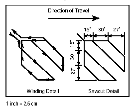
Figure 4-28. Type D loop configuration (Caltrans).
Figure 4-29 shows a Type D loop installation for detecting bicycles on a sidewalk or bicycle path. The wheel on the pole is used to push the wire into the sawcut and then to push foam backer firmly on top of the wire. There is debate about placing foam over the entire wire or simply using short foam pieces every foot or so. The first method supports easier installation from the contractor's perspective; the second provides better encapsulation by the sealant and less wire movement. |
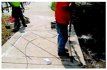
Figure 4-29. Type D loop installation (Photograph courtesy Darcy Bullock, School of Civil Engineering, Purdue University, West Lafayette, IN).
In some applications, it is desirable to detect the presence of a bicycle across a greater portion of a full-width traffic lane. Figure 4-30 shows one loop configuration suitable for this purpose, an 8-ft (2.4-m) square with three diagonal saw cuts traversing the square. Two layers of wire are used and are wound so that the current flow is in the same direction for both layers. This results in four layers of wire in each diagonal. The acute-angle corners are rounded to prevent damage to the wires. This is a special configuration that is installed in areas of heavy bicycle traffic such as near the University of California at Davis.
Figure 4-31 illustrates another method of reliable bicycle detection with two quadrupole loops placed side by side within the traveled area of a bike lane. An adjustable timed-call extension is generated to hold the call to the controller long enough for the bicycle to clear the intersection when operating in a loop occupancy mode. The 4.5- by 6-ft (1.4- by 1.8-m) configuration provides assurance of detecting all bicycles and complete adjacent lane rejection.
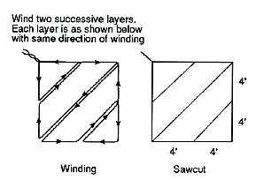
Figure 4-30. Wide coverage bicycle loop.
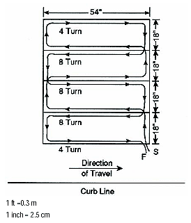
Figure 4-31. Bicycle lane loop layout with side-by-side quadrupoles.
It is generally advisable to allow long, high bed vehicles (e.g., tandem trucks, semitrailer trucks, and cars pulling trailers) to travel through the intersection without stopping. There are three good reasons why long vehicles should not be stopped:
A detection alternative for trucks consists of two loops spaced 30 ft (9 m) apart and located 302 ft (91 m) from the stopline.(17) This is the distance a loaded semitrailer vehicle traveling 45 mi/h (72 km/h) needs to stop safely. The sensor logic requires that the second loop be activated before the first loop is vacated.
The Detroit, MI, freeway program required that all vehicles be detected as a single entity, including high-bed trucks, semitrailers, and tanker trucks, as well as conventional vehicles. Their test of three-turn 6- x 6-ft (1.8- x 1.8-m) loops did not adequately satisfy their requirement. After numerous trials, the agency determined that a seven-turn 6- x 6-ft (1.8- x 1.8-m) loop rotated 45 degrees to form a diamond shape was superior particularly in its accuracy in detecting trucks. The diamond shape was further refined by carefully adjusting the angles of the diamond to avoid splashover.(25)
One manufacturer states that reliable truck detection from loop configuration change is not due to the diamond shape of the loop as suggested above. Rather it is due to the increased number of turns, which increases the inductance of the loop. The amount of signal received by the electronics unit is dependent on the loop inductance to lead-in cable inductance ratio. When the loop inductance to lead-in cable inductance ratio equals one, then the amount of change seen by the electronics units is one-half the change occurring in the loop. By increasing the loop inductance (by increasing the number of turns to seven), Detroit has greatly increased the amount of change received at the electronics unit, thereby resulting in more reliable detection of high-bed trucks.
Freeways that operate under congested conditions are periodically likely to experience heavy volumes on off-ramps. When these off-ramps terminate at a signalized intersection, backups can extend to the freeway lanes, causing even more congestion. Depending upon agency policy, it may be desirable to detect and discharge such queues before they become a freeway problem.
One solution uses an actuated controller with a queue-discharge system consisting of a queue sensor with a preset delay time.(13) As shown in Figure 4-32, the queue-detection loop is located at a strategic position at the upstream end of the off-ramp. A timer starts when a vehicle enters the detection zone of the queue sensor and resets to zero when the vehicle exits the zone of detection. If the system counts a predetermined number of seconds, i.e., the preset delay time, the electronics unit's normal output relay is energized.
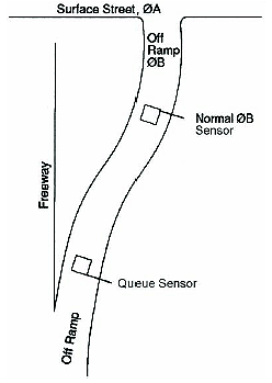
Figure 4-32. Queue discharge system.
If the queue of vehicles waiting at the red signal stopline extends upstream to the queue sensor, a vehicle will be located over the loop longer than the selected delay time. When the delay timer reaches the preset time, the sensor logic issues a signal to discharge the queue. The green signal remains on until all vehicles are moving with gaps longer than the loop itself.
The inductive loop must be long enough to span the distance between standing vehicles. Concomitantly, it must be shorter than the shortest gap in moving traffic so that the breaks between moving vehicles will cause the delay timer to reset. This latter consideration can be critical when a inductive-loop queue-sensor covers two or more lanes. A loop length of 30 ft (9 m) will generally satisfy this criterion.
The sensor requirements for area-wide traffic signal control systems are dependent on the type of control implemented. TOD control does not require detectorization as it operates as a time clock. First-generation traffic responsive control and other advanced control strategies require vehicle sensors capable of early identification of traffic trends within a system. The sensors must provide an early indication of a peak period for the beginning of heavy traffic. Thus, the sensors must be placed on heavily traveled links with traffic patterns representative of the significant flows within a section of the area-wide system.
The application of sensors to various arterial and freeway traffic management techniques was explored in chapter 3. Additional sensor design considerations for traffic-responsive traffic control systems are discussed below.
When sensor systems are used in computerized traffic-control systems, the particular traffic management application determines the traffic flow parameters to be collected and their accuracy. As discussed in chapter 3, volume and occupancy can be measured effectively. Other measured parameters may only provide approximations to the required variables, depending on how the data are gathered and subsequently processed. In estimating link-specific volumes, three components of error limit the measurement accuracy of each of the control variables. These are:
The data error can be expressed as X percent probability that the error is within Y percent. A normal distribution is assumed for the mean value of a large sample. The count error for first generation UTCS critical intersection control was plus or minus 3 vehicles 90 percent of the time.(18)
Several filtering and smoothing techniques may be applied to the data to calculate the values needed to produce measures of effectiveness that relate to traffic flow. A filtering equation determines the difference between the previous time period smoothed value (such as volume) and the latest unsmoothed value. The difference is used to update the value of the smoothed data.
Another error is introduced for vehicle presence because the controller does not generally observe vehicle presence continuously, but instead samples. This results in an error in occupancy and speed computations. There will always be a sampling error that increases as vehicle speed increases. This error cannot be eliminated but can be decreased by increasing the sampling rate. The Computerized Signal Systems Student Workbook(19) describes how to compute the percent sampling rate and how to implement filtering and smoothing techniques.
The location of sensors in a traffic-control system is a three-step process. First, links are selected for sensor installation. The lateral and longitudinal sensor placements are then determined. The link selection must consider each function in the sequence, beginning with intersections that are candidates for CIC. Candidate intersections are those that could take advantage of variable split, but which operate in an unsaturated condition. When installing sensors in an intersection to operate under CIC, all approaches served by phases with variable green times must be detectorized. The step-by-step process for determining CIC candidates is found in the Locating Detectors for Advanced Traffic Control Strategies Handbook.(20)
The need for measuring general traffic trends will probably be satisfied by the CIC sensors in area-wide surveillance systems. If this type of detectorization is not installed, sensors should be located on major collectors or distributors to the network to obtain system trends with a minimum of instrumentation. Another group of candidates for this type of detectorization are entrances and exits of large parking facilities that would have significant effects on local traffic conditions.
The location of sensors to evaluate system operation is, to a large extent, dependent upon the degree of accuracy required by the evaluation. If a general evaluation of changes in system operations is desired, the sensor placement for traffic responsive operation would be adequate. If a more detailed evaluation is required such that speed and delays can be determined, it is necessary to increase the number of sensors within the system. The cost of this amount of detectorization may suggest that other techniques be employed.
Observations have shown that a single vehicle sensor in the lane carrying the maximum through volume will be the most representative of the traffic to which the signal must respond. Moreover, the signal should be timed for critical lane volumes. However, it is not possible to derive reliable total volumes from a single sensor. Yet multiple inductive-loop detectors located in noncritical lanes may introduce errors that exceed the value of the data they provide as they can also measure parking vehicles, turning vehicles, etc., unless individual lane detection is used. Thus, the most reliable data are derived from the critical lane. The critical lane (defined as the one carrying the greatest volume) is usually easy to identify by observing the lengths of queues at the intersection.
Sensors should be installed in multiple lanes at locations where the critical lane changes with time of day, as should the corresponding TOD factors used in the software to select the inductive loop currently measuring the volume in the critical lane.
Traffic volumes should be measured on each lane of an intersection approach.(21) Average lane volumes per cycle need to be computed and compared with the tentative critical lane. Four conditions require engineering judgment pertaining to project priorities and knowledge of individual link traffic. These conditions are:
It is unusual for more than two lanes to require detectorization, and most often, only one lane will need a sensor. After the critical lanes have been identified for the links to be detectorized, it is necessary to determine the longitudinal placement of the sensors on the links.
There are two guidelines for the longitudinal placement of sensors for signal-system control. One relates to the upstream intersection, and the other refers to the downstream intersection. From the upstream intersection, a sensor should be downstream from the zone of acceleration of vehicles entering the link. A distance of approximately 230 ft (69 m) is recommended.
From the downstream intersection, the sensor should be upstream from the point beyond which standing queues of vehicles do not usually extend. Although this distance is a function of the cycle length, split, and offset, it is recommended that values of 200 to 250 ft (60 to 75 m) be used in urban grid areas and values of 300 to 350 ft (90 to 105 m) be used in suburban arterial systems. When both criteria cannot be met, the criterion based on typical queue size is considered the more critical.
An additional issue of longitudinal-sensor placement involves the location of traffic sinks and sources (e.g., parking facilities). Sensor placement research has shown that a sink or source has minimal effect on traffic measured in the critical lane when the facility is operated as a sink such as a parking garage during the morning peak. Turns into the garage are made from the curb lane, which is not usually the critical lane.
However, during the evening peak hour, when the garage functions as a source, there are measurable effects on the critical lane. An evaluation of the paths of vehicles entering the lane from a source showed that most vehicles wait for a sufficient gap to enter the specific lane within the link. It is suggested that a critical lane sensor be located at least 50 ft (15 m) downstream from the source, provided that the downstream intersection criterion is not violated. In general, unless the source contributes more than 40 vehicles per hour to the critical lane, the effects of a source on the link demand are not significant.
Sensor location information developed in earlier tasks assists in selecting links to be detectorized, lanes in which the sensor should be placed, and an approximate sensor location with respect to the upstream and downstream intersections. With this information indicated on a map, a field visit should be conducted for each link. A walk-through by the designer will permit the selection of final locations with consideration given to access to the control equipment, special driveway problems, or other roadway or parking conditions. Each sensor location must pass a reasonableness test as well as the analytical test.
Several general guidelines are suggested concerning the field location of individual inductive loops:
In summary, the final decision concerning the location of sensors for advanced traffic-control strategies is a blend of analytical procedures coupled with engineering judgment. Not all links can be instrumented to yield input measures within the accuracy required by the algorithms. Short links and links with extremely poor lane discipline are typical of those that are not compatible with accurate instrumentation.
The operational characteristics of various types of modern inductive-loop electronics units are discussed in detail in chapter 2. Requirements for inductive-loop electronics devices are included in the NEMA Standards and the Type 170 Specifications (see Appendices I and J). The NEMA Standards define a series of self-contained loop electronics units designed for shelf mounting. It also describes a card-type electronics unit designed to insert into a multicard housing rack. The revised NEMA Standards (TS-2) emphasize card-rack mounted units. The Type 170 Specifications define card-type modules only, which are designed for insertion into the input file of the cabinet system.
NEMA electronics units are available with one, two, or four independent inductive-loop detector channels per unit. Some agencies insist on using only single channel electronics units because they believe that failures in the unit can be more easily and inexpensively corrected by replacing a single channel unit rather than replacing a multiple channel unit for a single channel's failure. Current reliability of electronics units makes this argument obsolete. The rack-mounted modules used in the Type 170 system contain either two or four independent channels.
NEMA Standards also define optional timing features that allow for the delay or extension of the electronics unit output. In the delayed-call mode, the electronics unit will wait for a user-defined period after a vehicle enters the detection area before it starts the output signal. In the extended-call mode, the unit will extend the output after the vehicle leaves the detection area. The Type 170 electronics unit does not provide this capability, as extension is normally performed by software in the controller unit itself.
A magnetometer sensor system, such as the one shown earlier in Figure 2-39, consists of one or more magnetometer sensors, the magnetometer electronics unit, and the lead-in cable between the sensor and the electronics unit. The sensor probe installation is illustrated in Figure 4-33.
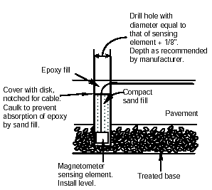
Figure 4-33. Conceptual magnetometer sensor installation.
Since the magnetometer is a passive device, there is no transmitted field or transmitted detection area. Modern magnetometer sensors detect changes in the horizontal and vertical components of the Earth's magnetic field caused by the passage or presence of a vehicle and, hence, can be used for either passage or presence detection as discussed in chapter 3.
Because the probes are buried in a drilled hole approximately 18 inches (0.5 m) below the surface, they find application in the northeastern United States , where the pavement deteriorates more rapidly due to thermal expansion and contraction and suffers damage from snow-removal equipment. They are also used in areas where loops cannot be cut in the road surface, such as on steel bridge decks.
The configuration for a magnetometer installation is dependent on a number of factors that must often be traded against one another when designing an optimum configuration for a specific location. The following section discusses these factors and their impact on the ultimate design.
Magnetometers will detect a vehicle whenever a sufficient portion of its magnetic shadow (i.e., changes in the horizontal and vertical components of the Earth's magnetic field caused by the passage or presence of a vehicle) falls on a sensor probe. The dimensions of the magnetic shadow generally approximate the geometric dimension of the vehicle. In some cases, the magnetic shadow may be offset from the probe by a few feet in any direction.
Electronics units for magnetometers provide two or more independent detection channels. Each channel supports 6 to 12 sensor probes, depending on the model. If only one probe per channel is installed in the street, the entire channel sensitivity is available to that single probe. However, as the number of probes per channel increases, the sensitivity is divided among the probes, thus decreasing the sensitivity of each individual probe. For example, when four probes are connected to a single channel, the total channel sensitivity remains the same, but the sensitivity at each probe will be reduced to one-fourth of the total channel sensitivity.
Therefore, it is necessary to determine what types of vehicles are to be detected in order to select the proper spacing between probes and to define the number of probes connected together per channel. The number of probes required per lane and their optimum cross-lane position are determined by the lane width and the size of the vehicles to be detected. Some portion of the vehicle must pass over a sensor probe to be detected. Some general guidelines for the number of probes for a given type of vehicle and the number of probes per channel are given below:
Installation sites should be chosen to avoid conditions that adversely affect operation such as those adjacent to manholes or large pipes; near very high current transmission lines, trolley lines, or underground power lines; or within tunnels or other iron-structure enclosures.
Magnetometers are frequently the sensor of choice on bridge decks. Figure 4-34 illustrates a typical bridge deck installation. The presence of the steel deck over or under the probe has little effect on system performance. However, vertical structural steel members may detract from performance by reducing the intensity of the adjacent ambient magnetic field. As with loops, the most appropriate location for the probes is at the maximum distance from the steel supports or columns as shown in the illustration.
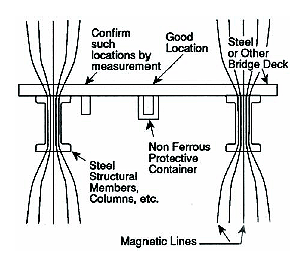
Figure 4-34. Typical installation of magnetometers on a bridge deck.
A magnetic field analyzer, such as the model shown in Figure 4-35, should be used to measure the intensity of the magnetic environment at the selected location. This instrument measures geomagnetic field intensity, magnetic noise, and ac magnetic field strength. It is especially useful at locations where the use of magnetometers is questionable (e.g., within tunnels, near large electrical devices, etc).
Situations exist where manmade magnetic noise is of sufficient intensity to impair magnetometer performance. These occur at sites where nonvehicular induced magnetic field perturbations exceed 5 milliOersteds such as near streetcar lines, some trolley bus lines, subway trains, or even elevators. Few sources are of sufficient intensity to affect a sensor probe located more than 30 ft (9 m) from the source. However, magnetometers that transmit data via a radio frequency link to the electronics unit in the controller cabinet are subject to interference from communications devices operating at the same frequency. Therefore, a frequency survey should be performed to determine a clear channel on which to transmit these magnetometer data.
The optimum lateral placement of probes in a lane is determined by such factors as the width of the narrowest vehicle to be detected, the lane width, and the detection quality required. Some part of the magnetic shadow of the vehicle must fall on one or more of the probes for detection to occur. Consequently, the maximum probe spacing is equal to the width of the narrowest vehicle to be detected. Since most autos, trucks, and buses are wider than 5 ft (1.5 m), a single probe centered in a 10-ft (3-m) lane provides adequate performance. In a 12-ft (3.7-m) lane, a single probe may fail to detect some small vehicles traveling on the edge of the lane.
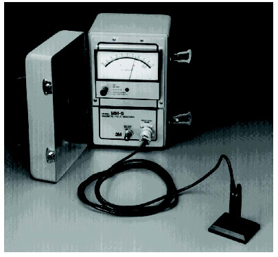
Figure 4-35. Magnetic field analyzer.
By increasing the number of probes to two per lane, virtually all four-wheeled vehicles within a 12-ft (3.7-m) lane would be detected. In this type of configuration, probes should be placed no further than 5 ft (1.5 m) from each lane boundary. If bicycles are to be detected, more probes per lane may be needed.
In general, the quality of detection improves as the number of probes per lane is increased because of the spatial averaging, which results when the magnetic shadow of a vehicle falls on several probes judiciously spaced. Reduction in field intensity at one lateral position may be compensated for by increases at other positions.
Vertical placement of probes is an important determinant of system performance properties. Deep placement such as 18–24 inches (45–60 cm) provides good single-count vehicle-presence detection, but results in a lower signal level. Conversely, shallow placement (e.g., 6 inches (15 cm)), provides higher signal levels, but with an increased incidence of multiple counts per vehicle. Multiple counts with shallow placement result primarily from the passage of major components of the vehicle such as engine, transmission, and differential, each of which may produce a separate magnetic perturbation. By increasing the depth to 18–24 inches (45–60 cm), most vehicles yield a single perturbation of the magnetic field because the deeply buried probes sense the overall magnetic bulk of the vehicle rather than details of the understructure.
In summary, for a detection application where only passage information is required and where multiple counts are not detrimental, probes should be located near the surface. Similarly, in constant speed applications where the time-extension feature of the extendable-presence mode can be used effectively, probes may be located near the surface. Small, two-wheeled vehicles such as bicycles or motorbikes develop narrow, low-intensity shadows. Their detection requires shallow placement of probes, as well.
Different probe placements and connections to the electronics unit are used to support various traffic management functions and data acquisition needs as depicted in Figure 4-36. Several typical probe configurations are presented in Appendix L. These illustrate the tradeoffs made in probe depth and lateral distance between probes. Configurations are included for single-lane, two-lane, and three-lane detection; wide-lane detection; and two-wheeled vehicle detection. Also shown are several suggested configurations for left-turn lanes with detection zones ranging from 30 to 70 ft (9 to 21 m).
Cable length and number of probes per channel determine minimum wire size. The probe excitation circuit provides current at a constant 125 mA peak-to-peak, but is limited to a 15-volt peak-to-peak swing. Maximum allowable probe-cable assembly resistance is therefore 125 ohms. At resistance levels below this limit, system operation is normal. At higher resistance levels, instability and performance degradation will occur.
Effective resistance of each probe is approximately 4 ohms. Probes on a channel are connected in series electronically, so their resistance is additive. Allowable cable resistance is 120 ohms, less the sum of the probe resistances. AWG #22 copper wire pairs have a loop resistance (going and returning total) of 35 ohms per l,000 ft (300 m), AWG #20 pairs have 20 ohms, and AWG #18 pairs have 13 ohms. Because of the changes in wire resistance with temperature, it is recommended that #18 AWG wire be used on cable runs exceeding 2,000 ft (600 m) in climates where extreme temperature ranges are typical.
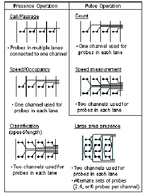
Figure 4-36. Magnetometer-probe placement in support of several data-gathering functions.
Connection of the magnetometer electronics unit and probes requires two pair of conductors per channel. One pair supplies the probe excitation current and the other carries the return signal. Properties of the cable become especially significant in long transmission distances of over 2,000 ft (600 m). The cables should combine distance capability with high noise immunity and environmental tolerance.
Although up to 12 probes per channel can be installed, the allowable lead-in length decreases as the number of probes increases. Generally, the lead-in length should not exceed 4,000 ft (1,200 m) for a 12-probe-per-channel arrangement. If 6 probes per channel are used, the lead-in length should not exceed 5,000 ft (1,500 m).
Magnetic detectors first developed in the 1930s, i.e., sensors whose operation is based on an induction magnetometer (also referred to as a search coil magnetometer), are still in use today, particularly where deteriorated pavement or frost activity contributes to the failure of inductive-loop detector wires. Magnetic detectors are also applied where vehicle detection is required without placing sawcuts in the pavement. While magnetic detectors are inexpensive, reliable, and simple, most generate only pulse outputs, which are suitable in support of traffic actuated signal control and traffic volume counting. The exception is the Model 702 microloop probe from 3M, which can be connected in rows of three to detect stopped vehicles with application-specific software purchased from the microloop manufacturer.
The magnetic detector contains a coil of wire wound around a highly permeable core, which is placed below the surface of a roadway. When a ferrous metal vehicle comes near or passes over the coil, the lines of flux produced by the Earth's magnetic field that pass through the coil are perturbed by the vehicle, thus inducing a voltage in the coil. A high-gain amplifier boosts this voltage to operate a relay, which sends a signal to the controller that a vehicle has been detected.(22)
The following discussion is limited to the induction magnetometer or magnetic detector. The model shown in Figure 2-42 is cylindrical in shape, 2.25 inches (57 mm) in diameter and 21 inches (533 mm) long.
Probe placement is critical for the proper operation of this sensor system. For the probe to detect a change in the Earth's magnetic field, a vehicle must be moving at a speed greater than approximately 5 mi/h (8 km/h). This implies that the probe must be placed far enough back from the stopline where vehicles are normally in motion (generally at least 50 ft (15 m)). It must also be placed in the most appropriate location across the lane to generate a sufficiently strong signal to register a vehicle detection.
The setback distance of the probe from the stopline is based on the desirable allowable gap. Assuming an allowable gap (or equivalently, a passage time) of 3 seconds, the probe would be located 132 ft (40 m) from the stopline on a street with vehicles traveling at 30 mi/h (48 km/h). The graphs shown in Figure 4-37 identify the proper location of the probe relative to the stopline based on allowable gaps of 2, 3, 4, or 5 seconds.
In a single-lane approach to a stopline, the optimal location of the probe is under the path normally followed by the right wheels of the vehicle, as shown in Figure 4-38. On a two-lane approach where a single probe is used, the probe is placed between the lanes to provide satisfactory coverage. If the right lane of a multilane approach is designated for right-turning traffic, the probe is located in the middle of the through lane to minimize the effect of vehicles in the right-turn lane.
A common practice for multilane approaches is to place a probe in each lane. In such designs, the probe is placed under the right wheel track in each lane. Up to three probes can be placed in a conduit. When magnetic probes are placed in a new roadway, multiple conduits should be used, one probe per conduit. In an existing road, conduit runs should be kept to a minimum; thus, more than one probe may be placed in a conduit.
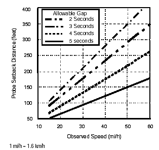
Figure 4-37. Setback of magnetic probe from stopline as a function of vehicle speed and allowable gap.
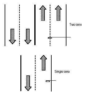
Figure 4-38. Magnetic probe placement for a single-lane and two-lane approach to a stopline.
Two or more probes used on different approaches of the same traffic phase should be placed in similar locations (if possible) so that the area monitored by each probe is the same. This permits the sensitivity of all sensors to be adjusted by the single sensitivity-adjusting knob.
A sensor probe generates an impulse in response to any change in the magnetic conditions surrounding it. The impulse strength is proportional to the change in the magnetic field. Changes in the magnetic field can be caused by movement of iron or steel objects in the vicinity of the probe or by changes in the current flowing through power lines. With the probe placed as close as possible to the path of the vehicles, the strength of the impulses caused by these vehicles will be maximized. Impulses caused by traffic moving in other lanes or by current changes in nearby power lines will be minimized. The sensitivity of the sensor can be decreased until the unwanted impulses are reduced in strength so that they do not actuate the relay, while the impulses from vehicles in the proper lanes remain strong enough to cause actuation.
FHWA-HRT-06-108

