U.S. Department of Transportation
Federal Highway Administration
1200 New Jersey Avenue, SE
Washington, DC 20590
202-366-4000


Skip to content
Facebook iconYouTube iconTwitter iconFlickr iconLinkedInInstagram

Federal Highway Administration Research and Technology
Coordinating, Developing, and Delivering Highway Transportation Innovations

Report
This report is an archived publication and may contain dated technical, contact, and link information
Publication Number: FHWA-HRT-04-095
Date: November 2004

Manual for LS-DYNA Soil Material Model 147

PDF Version (1.96 MB)

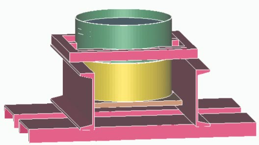
PDF files can be viewed with the Acrobat® Reader®

CHAPTER 3. EXAMPLES MANUAL

This section presents some examples of simulations that were used during the verification phase of the development of the FHWA soil material model. The first example can be used to check the model accuracy and to familiarize the user with the material model. It consists of a single-element simulation of a triaxial compression experiment. Appendix B contains an example of the input for the triaxial compression single-element simulation. Figure 27 shows the results of the single-element simulation of a triaxial compression test at 3.4 MPa.

Figure 27. Z-stress versus time for single-element 3.4-megapascal triaxial compression simulation. Graph. This figure shows one red line labeled element number A1. The vertical axis of this graph ranges from negative 0.016 to negative 0.002 and represents stress, while the horizontal axis of this graph ranges from 0 to 100 and represents time. The red line begins at the top of the graph, at the point of negative 0.000 and descends toward the horizontal axis. The letter A is placed at the points of negative 0.006 on the vertical axis and 20 on the horizontal axis, where the line continues to descend. Another letter A is placed at the point just below negative 0.014 on the vertical axis and just before the point of 40 on the horizontal axis, where the red line plateaus and runs parallel with the horizontal axis until it leaves the graph. The letter A is also placed along the horizontal line at the points of 60, 80, and 100 on the relative axis.

Figure 27. Z-stress versus time for single-element 3.4-MPa triaxial compression stimulation.

The peak strains in this example reach 80 percent. This shows that the material model will successfully analyze problems with large strains (deformations).

A second example of the use of the FHWA soil material model is a simulation of a direct shear test. The goal of the tests was to determine the soil properties for the NCHRP Report 350 strong soil using large test specimens. The analysis is of direct shear test 4 (DS-4).(16) Contractors developed the model (see figure 28). The material model input for this simulation is shown in appendix B. Figure 29 shows the comparison between the test and the analysis of shear force versus deflection. The early time test data exhibit questionable trends and the analysis results show the expected trend (i.e., positive stiffness). Figure 30 shows the deformed shape of the cylinder at the end of the analysis. The analysis was terminated at approximately 47 millimeters (mm) of deflection because of the current failure criteria in LS-DYNA. An element fails (i.e., is eliminated from the simulation) when one of the gauss points reaches the failure criteria. For selective reduced integrated elements (8 gauss points), this causes premature failure. This premature failure does not let the internal forces go to zero in the failed elements. In turn, this leads to very large unbalanced forces at the nodes, causing unstable behavior (shooting nodes).

Figure 28. LS-DYNA model of direct shear test DS-4. Image. This figure shows a cylinder contained inside a rectangular collar with the front of the collar removed. The collar rests on two separate beams running parallel with each other. With the front of the collar removed, the entire cylinder is visible. The lower half of the cylinder is colored yellow, while the top half of the cylinder is green.

figure 28 LS-DYNA model of direct shear test DS-4.

The element formulation for this model is selective-reduced (S/R) elements. It is well known (see note 5 in the *SECTION input of the LS-DYNA manual) that poor aspect ratios (highly distorted elements) will cause shear locking. Elements along the shearing surface of the direct shear test simulation experience very large distortions, approximately equal to the element dimensions. Therefore, if severely distorted elements are not eliminated by erosion, the simulation will produce excessively stiff response (shear locking). An obvious way to overcome these problems is to use the standard constant stress (1 gauss point) element. However, time and funding did not allow the exploration of this option. A second option would be to refine the element mesh in the vicinity of the shearing surface to reduce the large deformations of the individual elements. A third option would be to use the Arbitrary Langrangian-Eulerian (ALE) formulation and the constant stress element. However, at this time, the FHWA material model is not available for use with ALE (although the capability of the FHWA soil material model to be used in conjunction with ALE was successfully tested during the early phase of this development effort with the model implemented as a user-defined material model).

As shown in figure 30, there are surfaces of the soil, which at the time of the analysis, are in contact with the metal or air. Also, the interface between the two cylinder halves has become a noncontinuous surface (i.e., a slide surface). This behavior cannot be accurately modeled by the continuum mechanics material model; it must be modeled by slide surfaces.

Figure 29. Shear stress versus deflection comparison for DS-4. Graph. This graph compares shear stress versus deflection results from an LS-DYNA calculation with similar results from direct shear test DS-4. This graph shows two curves, one blue, depicting results of the LS-DYNA calculation, and the other red, depicting test data DS-4. The vertical axis of this graph ranges from 0 to 60 and represents shear stress in kilopascals, while the horizontal axis of this graph ranges from negative 1.00E plus 01 to 8.00E plus 01 and represents deflection in millimeters. The LS-DYNA curve rises from 0 to a peak of about 53 kilopascals at 37 millimeters deflection, followed by a reduction in stress to 44 kilopascals at 47 millimeters. The test data curve rises from 0 to a peak of about 44 kilopascals at 17 millimeters, then decays gradually to 32 kilopascals between 44 millimeters and 75 millimeters deflection.

Figure 29. Shear stress versus deflection comparison for DS-4

Figure 30. Analysis results for DS-4 deformation. Image. This image shows two rectangular blocks running lengthwise. One is off-center on top of the other, and they are separated by a thin red line. The top block is a green hue; the color is darkest at the left side, it fades moving in toward the center of the block, then it darkens again as it moves toward the right side of the image. There are a few white scratches on the right side of the block. The block below is identical, with the exception that the hue is yellowish and there are no scratches on its surface.

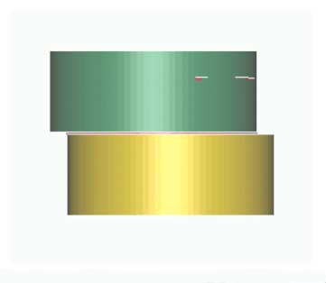
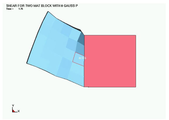
Figure 30. Analysis results for DS-4 deformation

As shown in figure 30, there are surfaces of the soil, which at the time of the analysis, are in contact with the metal or air. Also, the interface between the two cylinder halves has become a noncontinuous surface (i.e., a slide surface). This behavior cannot be accurately modeled by the continuum mechanics material model; it must be modeled by slide surfaces.

Figure 31. Simple two-material shear model. Image. This figure shows a rectangular image separated equally in two halves; the left half is shaded light blue, and the right half is shaded a dark pink. There is a square on the left side of this image, centered along the split line and outlined in red against the light blue background. Inside this box, the figure 'H 115' is written in white. This rectangular image is surrounded by an even larger rectangular image with an extremely pale blue background. In the top left corner of this image, the title 'Shear for Two Mat Block' is written with 'Time equals 0' written below it. The bottom left corner of this image contains a small right angle with the vertical axis labeled Y and the horizontal axis labeled X.

Figure 31 Simple two-material shear model.

The input parameters for the soil material were from the direct shear analysis. Figure 32 shows the deformed shape of the 1 gauss point element analysis at 1.75 milliseconds (ms), and figure 33 shows the deformed shape of the 8 gauss point element analysis at 1.75 ms. The analyses were stopped just before the 8 gauss point element becomes unstable because of the failure criteria error in the 8 gauss point element (outside the material subroutine).

Figure 34 shows the x-y shear stress in element 115 (shown in the previous figures). Since the soil material has a low cohesion (shear strength at zero normal force) of 6.2 x 10⁻⁶ gigapascals (GPa) (6.2 kilopascals (KPa)), the x-y shear stress should not get very large. The 8 gauss point element shows an immediate increase in the x-y shear stress to more than 0.03 GPa (30 MPa); this type of behavior is known as "shear locking." It is caused by the formulation of the 8 gauss point element outside of the material routine. As mentioned previously, this inaccurate behavior is mentioned in the LS-DYNA manual. The 8 gauss point element should not be used for any analysis that involves shearing or failure.

Figure 32. Deformed shape of 1 gauss point element analysis image. This figure shows a rectangular image separated equally in two halves; the left half is shaded light blue, and the right half is shaded a dark pink. The left half of the rectangle has been pulled upward in an arching fashion, warping that half of the image. There is a square on the left side of this image, centered along the split line and outlined in red against the light blue background, though the square has been elongated due to the unconventional form of the larger image, with its upper left hand corner pulled upward. Inside this box, the figure 'H 115' is written in white. This rectangular image is surrounded by an even larger rectangular image with an extremely pale blue background. In the top left corner of this image, the title 'Shear for Two Mat Block' is written, with 'Time equals 1.75' written below it. The bottom left corner of this image contains a small right angle with the vertical axis labeled Y and the horizontal axis labeled X.

Figure 32. Deformed shape of 1 gauss point element analysis.

Figure 33. Deformed shape of 8 gauss point element analysis. Image. This figure shows a rectangular image separated equally in two halves; the left half is shaded light blue, and the right half is shaded a dark pink. The left half of the rectangle has been pulled upward even further in an arching fashion, warping that half of the image. This half of the image is also speckled with darker squares of blue close to the separation line of the image. In addition, the outline of this half of the image is darkened and is more pronounced, almost giving the image a three-dimensional appearance. There is a square on the left side of this image, centered along the split line and outlined in red against the light blue background, though the square has been elongated due to the unconventional form of the larger image, with its upper left corner pulled upward. Inside this box, the figure 'H 115' is written in white. This rectangular image is surrounded by an even larger rectangular image with an extremely pale blue background. In the top left hand corner of this image, the title 'Shear for Two Mat Block' is written with 'Time equals 1.75' written below it. The bottom left corner of this image contains a small right angle with the vertical axis labeled Y and the horizontal axis labeled X.

Figure 33. Deformed shape of 8 gauss point element analysis.

Figure 34. Comparison of X-Y stress at element 115 for 1 gauss point and 8 gauss point elements. Graph. This graph compares shear stress versus time results from two LS-DYNA calculations. One calculation was conducted with one gauss point. The other calculation was conducted with eight gauss points. The vertical axis of this graph ranges from negative 0.035 to 0.005 and represents XY-shear stress in gigapascals, while the horizontal axis of this graph ranges from 0 to 2 and represents time in milliseconds. The maximum shear stress calculated with one gauss point remains effectively zero over time, while the maximum shear stress calculated with eight gauss points increasing nonlinearily with time to a maximum of about negative 0.033 gigapascals.

Figure 34. Comparison of x-y stress at element 115 for 1 gauss point and 8 gauss point elements.

The material properties used in the simulations/examples described above were not determined from actual material property test data, but were found by trial and error. Obviously, actual material property data would probably lead to more confident results.

Previous | Table of Contents | Next

Federal Highway Administration | 1200 New Jersey Avenue, SE | Washington, DC 20590 | 202-366-4000
Turner-Fairbank Highway Research Center | 6300 Georgetown Pike | McLean, VA | 22101