• Federal Highway Administration >
• Publications >
• Research Publications >
• 04096 >
• 5.Cfm >
• Evaluation of LS-DYNA Wood Material Model 143

Evaluation of LS-DYNA Wood Material Model 143

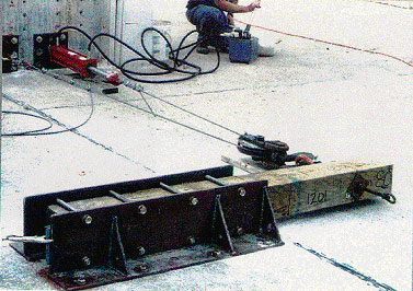
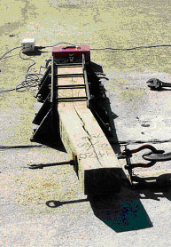
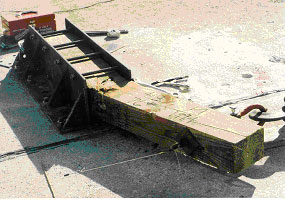
PDF files can be viewed with the Acrobat® Reader®

5 - Quasi-Static Post Test Correlations

The main reason for developing the wood material model is to analyze wood posts in roadside safety applications. Such posts are often saturated. Although the FPL data discussed in the preceding sections are useful for model evaluation and input parameter selection, the data focus on dry timbers rather than saturated wood posts. Therefore, additional bending test correlations are reported here for saturated wood posts.

The main objective for simulating the user’s quasi-static tests is to select specific default parameters, namely, quality factors and parallel-to-the-grain fracture energies, as a function of grade. The user’s test data are reviewed first, followed by correlation of the LS-DYNA simulations with the test data. Finally, the results from a number of parametric studies are reported.

5.1 - Southern Yellow Pine Bending Test Data

The user conducted 25 bending tests on southern yellow pine posts of three grades (DS-65, 1D, and 1).⁽⁷⁾ The grading was performed without considering waning on the ends of the posts. The posts were removed from the field from guardrail installations throughout Nebraska. They were cantilevered in a rigid frame and were loaded at a constant rate (as shown in figure 7). In some tests, neoprene and steel were wedged between the wood post and the steel support (as shown in figure 8). Load and deformation were continuously recorded. All post failure was dominated by tensile failure of the growth rings.

Figure 7. Quasi-static post test setup.

(a) Steel at bottom of support	(b) Neoprene at top of support on compression side
Figure 8. Details for the rigid frame used in the quasi-static post test setup.

Peak force, deflection, and energy are listed in table 1. Moderate scatter is observed in the data. For the grade 1 and DS-65 posts, all peak-force measurements are within 20 percent of the average measurements. For the grade 1D posts, all peak-force measurements are within 33 percent of the average measurement. For example, for grades 1 and 1D posts, peak forces range from 24.0 to 72.5 kilonewtons (kN) and deflections at peak force range from 30.5 to 94.0 mm. For DS-65 posts, peak forces range from 53.8 to 77.8 kN and deflections at peak force range from 43.2 to 91.4 mm.

Table 1. Average of static post test data by grade.

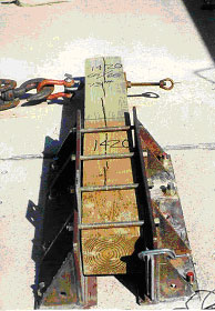
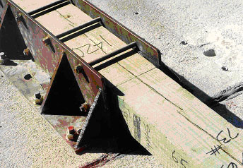
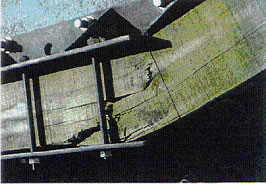
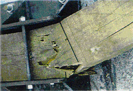
Deformed configurations from one grade DS-65 and one grade 1 southern yellow pine specimen are given in figure 9. Closeup views of damage in the break region are given in figure 10. Example load-deflection histories are given in figure 11. The curves exhibit slight pre-peak nonlinearity, followed by sudden drops in load as the specimens fail in the tensile region.

(a) DS-65 test 1420	(b) Grade 1 test 418
Figure 9. Deformed configurations of posts in static tests.

(a) DS-65 post	(b) Grade 1D post
Figure 10. Closeup of damage observed in break region of posts in static tests.

Figure 11. Measured load-deflection histories exhibit
sudden drops in force as the post fails in the tensile region.

The user developed performance envelopes from quasi-static load-deflection and energy-deflection curves. These envelopes are shown in figure 12, along with the performance envelopes developed from the dynamic bogie impact tests (to be discussed later). The user constructed the envelopes using curves from posts that exhibited the most typical behavior. For example, the DS-65 performance envelopes were developed from 6 of the 10 tests reported in table 1. The grade 1 performance envelopes were also developed from some, but not all, of the 15 tests reported in table 1. The grade 1 performance envelopes represent the combined curves from the grades 1 and 1D tests because the behavior of the grades 1 and 1D posts was similar. Note that the minimum and maximum curves that define the performance envelopes do not represent any one particular curve from the tests.

Measured curves plotted by the user are reproduced in figure 13 for grades 1 and 1D. Showing all of the curves allows us to better see the character of the data (such as scatter and sudden drops in force). This is important because the static post test analyses performed by the developer, which are discussed in the next section, exhibit large variations in post-peak behavior and sudden drops in force. A comparison of the performance envelopes in figure 12 with the measured data curves in figure 13 suggests that the static performance envelopes are developed from data that exhibit the largest fracture energies.

The relatively small scatter of the performance envelopes is surprising, especially considering that the failure (softening) curves are being measured. For example, see the scatter in the data measured by FPL for their timber compression and bending tests in figures 5 and 6. The reader is also referred to appendixes A and B of the wood model user’s manual⁽²⁾ for plots of clear wood stiffness and strength measurements. Clear wood stiffnesses (and strengths) vary by a factor of three from high measurement to low measurement.

5.2 - LS-DYNA Correlations

Multi-element simulations of guardrail posts in bending were performed at two grade levels for comparison with the performance envelopes (as shown in figures 14 and 15). Good correlations in the loading region primarily determine the tensile and compressive quality factors. The compressive quality factor also has a significant effect on the late-time softening response. The quality factors selected were Q_T = 0.47 with Q_C = 0.63 for grade 1 posts, and Q_T = 0.80 with Q_C = 0.93 for DS-65 posts.

Good correlations in the post-peak softening region determine the parallel-to-the-grain fracture energies. Parallel fracture energies (G_{f II}) are reported here as multiples of the perpendicular fracture energies (G_f ). Fracture energies used in these simulations are G_{f II} = 250 G_f kN-mm for grade 1 and G_{f II} = 380 G_f kN-mm for DS-65, with B = 30 for both grades.

Deformed configurations at 200 milliseconds (ms) (approximately 190 mm) are shown in figure 16, along with fringes of damage. The damage plotted is the maximum of the parallel and perpendicular damage. High damage (greater than 80 percent) is indicated by the red elements.

(a) Force versus deflection (b) Energy versus deflection

Figure 14. Good correlations between the LS-DYNA calculations and quasi-static performance envelopes determine the default quality factors for grade 1 southern yellow pine of QT = 0.47 with QC = 0.63.

(a) Force versus deflection (b) Energy versus deflection

Figure 15. Good correlations between the LS-DYNA calculations and quasi-static performance envelopes determine the default quality factors for DS-65 southern yellow pine of QT = 0.80 with QC = 0.93.

(a) Grade 1 deformed configuration	(b) Fringes of damage
(c) DS-65 deformed configuration	(d) Fringes of damage
Figure 16. The parallel-to-the-grain post fracture calculated in the post just below the top of the rigid support is in agreement with the location of the damage observed in the tests.

Details for the geometric models and parametric calculations used to establish these default parameters are given in the following section.

5.3 - LS-DYNA Parametric Studies

Various parametric calculations were conducted to further evaluate the material model and default material property selection.

Meshing: The parametric calculations were performed with three geometric models as shown in figure 17. The first geometric model uses fixed nodal constraints, without the use of slide surfaces. Neither the steel support nor the loading bolt is modeled. Therefore, it is the fastest running model. The second geometric model uses planar rigid walls of a finite size to model the steel support. The slide surface between the wood post and the rigid wall is modeled with a coefficient of friction of 0.30. In addition, the steel loading bolt is explicitly modeled. The third geometric model explicitly meshes the steel support as brick elements of rigid material. This mesh was developed by the user.

(a) Fixed nodes	(b) Rigid walls	(c) Full-support structure
Figure 17. Three geometric models were set up for performing parametric calculations.

Load-deflection curve comparisons are given in figure 18 for the full-support and rigid-wall models. Behaviors are similar, as though the load-deflection curve of the full-support model is shifted relative to the rigid-wall model. All default quality factors were selected from final calculations performed with the full-support structure. However, most parametric calculations were performed with either the rigid-wall model or the fixed-node model. This is because the rigid-wall model runs 15 times faster than the full-support model, while the fixed-node model runs 45 times faster than the full-support structure. Unless otherwise stated, all parametric calculations reported in this section are conducted with the rigid-wall model.

(a) Force deflection	(b) Energy deflection
Figure 18. The force-deflection curve calculated with the fast-running, rigid-wall model is similar to that calculated with the full-support structure, making it useful for performing parametric calculations.

Loading Method and Rate: The method of loading the bolt has a minor effect on the calculated response. This is demonstrated in figure 19(a) for two loading methods. In the first method, horizontal velocity is applied to the rigid bolt (or post). This means that no vertical forces are applied to the bolt, so the post is free to rotate. In the second method, horizontal velocity is applied to the end of a truss that is pinned to the bolt (as shown in figure 19(b)). This means that small vertical forces are applied to the bolt to simulate the effect of the pulley system on post rotation. The pulley system of the test configuration was previously shown in figure 7. It was used to load the bolt attached to the wood post. Application of the pinned truss increases the peak force by about 4 percent. All default parameters were selected from calculations performed with the truss. The calculations previously shown in figure 18 were performed with a truss.

(a) Load-deflection comparisons	(b) Rigid-wall mesh with truss
Figure 19. Pinning a truss to the bolt to simulate the vertical force applied by the pulley system increases the peak force by about 4 percent.

The calculations are intended to simulate static tests, so the rate of loading must be slow enough to eliminate dynamic oscillations that can initiate premature damage and plastic hardening. This is achieved by ramping the applied velocity (to the post or truss) from zero to a constant sustained value over a 15-ms interval. Clear wood calculations performed with the simplest (fixed nodes) mesh are compared in figure 20 for sustained velocities of 1.0 and 0.25 meters per second (m/s). The calculated load-deflection curves are quite similar, particularly the peak force. All default parameters were selected from calculations performed at 1.0 m/s.

Figure 20. The peak force increases with the applied
velocity until convergence is attained at 0.25 mm/ms.

Filtering: All static computational force histories are also post-processed using the Society of Automotive Engineers (SAE International) 60 filter in LS-TAURUS (an LS-DYNA post-processor) to remove the high-frequency post-peak oscillations that occur as the elements soften in the tensile region. A different filtering method is used for the bogie impact calculations discussed later. Filtering is used because it is not practical to run the calculations slow enough to eliminate all post-peak oscillations; the calculations are quasi-static rather than static. The filtering primarily clarifies the post-peak softening response for comparison with the unfiltered test data. One comparison between clear wood calculations, with and without filtering, is shown in figure 21. These calculations were performed with the simplest (fixed nodes) mesh.

Figure 21. Quasi-static calculations are filtered for
easier comparison with the unfiltered test data.

Fracture Energy: The calculated response depends on the value of the parallel-to-the-grain fracture energy. Comparisons at two different fracture energy levels are shown in figure 22. The greater the parallel fracture energy, the more gradual the post-peak softening response, and the more energy it takes to break the post. These comparisons were performed with B = 30, and Q_T = 0.47 with Q_C = 0.63.

The two values used in the simulations are G_{f II} = 250 G_f kN-mm and G_{f II} = 50 G_f kN mm for grade 1. Here, G_{f II} is the parallel-to-the-grain fracture energy and G_f is the perpendicular-to-the-grain fracture energy. The 250 value is obtained from correlations with the static performance envelopes. The 50 value is obtained from correlations with the dynamic performance envelopes (discussed in subsequent sections). Although the peak forces are similar, the post-peak response is substantially different. The calculation conducted with G_{f II} = 50 G_f kN-mm does not fit within the performance envelopes; however, it does correlate well with the suite of measured data previously plotted in figure 13. In this figure, 9 out of 15 of the data curves peak between 25 and 50 mm of deflection and then exhibit a sudden drop in force. The calculation is consistent with the measured behavior.

Figure 22. The energy required to break the post increases as
the value of the parallel-to-the-grain fracture energy increases.

Compressive Quality Factor: For a given fracture energy, the softening response also depends on the compressive quality factor. Two computational comparisons are shown in figure 23. The calculation with Q_T = Q_C = 0.60 gives approximately the same peak force as the calculation with Q_T = 0.47 with Q_C = 0.63, but does not soften as rapidly. Numerous parametric calculations have demonstrated that increasing the value of Q_C above Q_T increases the force at the peak, but decreases the force at a large deflection (reduces the tail). This is because yielding in the compressive region is delayed by increasing Q_C. Allowing Q_C to be greater than Q_T is consistent with our fits to the FPL static bending test data previously shown in figure 6. All default quality factors were selected with Q_C greater than Q_T.

(a) Force deflection	(b) Energy deflection
Figure 23. Calculations with QC > QT soften more rapidly than calculations with QC = QT.

Softening Shape Parameter: The calculated response also depends on the value of the softening parameter B (as shown in figure 24). The greater the value of B, the greater the peak force. Recall that the parameter B determines the shape of the softening curve in single-element simulations. This is shown in figure 25 for tension parallel to the grain. A moderate value of B = 30 was selected for use as a default parameter. This value is somewhat arbitrary because no softening-curve measurements are available from the FPL direct-pull simulations for fitting the softening model. Softening curves are often difficult to measure. These clear wood calculations were performed with the simplest mesh at 1 m/s using G_{f II} = 300 G_f .

Figure 24. The calculated peak force increases with
increasing values of the softening parameter B.

Figure 25. The softening parameter B determines the shape of the softening
curve in these single-element simulations for tension parallel to the grain.

Hourglass Control: The calculated response also depends on the hourglass control. To demonstrate this, calculations performed with viscous and stiffness hourglass controls are compared to a calculation performed with selectively reduced (S/R) integrated elements (ELFORM 2 is called a fully integrated S/R solid). Deformed configurations in the break region are shown in figure 26. Load-deflection curves are shown in figure 27. Hourglass energy histories are shown in figure 28.

The simulation with viscous hourglass control exhibits hourglassing at an early time, resulting in an unrealistic pinching behavior on the backside of the post in the compressive region near ground level. Hourglassing is concentrated in the breakaway region of the post, where the damage accumulates. Type 3 viscous control, with a default coefficient of Q_M = 0.1, was used throughout the post breakaway region. The simulation with stiffness hourglass control exhibits less visual hourglassing and pinching. Type 4 stiffness control, with a reduced coefficient of Q_M = 0.005, was used throughout the post breakaway region. The third simulation was performed with fully integrated elements (eight integration points) in the breakaway region. Fully integrated elements do not require hourglass control. Note that the deformed configuration and the peak force calculated with stiffness hourglass control are in best agreement with those calculated with the fully integrated elements.

One common concern is that stiffness hourglass control overstiffens the calculated response. These comparisons indicated that stiffness hourglass control does not stiffen the calculated response unrealistically. In fact, the calculation with stiffness control matches the peak force calculated with fully integrated elements. In addition, the final hourglass/internal energy ratio in the breakaway region is slightly less with stiffness control than with viscous control. Therefore, stiffness hourglass control with Q_M = 0.005 was used in the breakaway region of all calculations involving default parameter selection. As a bonus, the calculation with stiffness control runs the fastest. The viscous control and fully integrated element calculations run 7 percent and 51 percent longer, respectively, than the stiffness control calculation.

(a) Viscous control	(b) Stiffness control	(c) Fully integrated S/R
120-mm deflection
(d) Viscous control	(e) Stiffness control	(f) Fully integrated S/R
190-mm deflection
Figure 26. Type 4 stiffness control reduces hourglassing better than type 3 viscous control.

Figure 27. The peak force calculated with type 4 stiffness control agrees with the
fully integrated element calculation better than the type 3 viscous calculation.

Figure 28. Less final hourglass energy is calculated with
type 4 stiffness control than with type 3 viscous control.

Moisture Content: Moisture content has a strong effect on the calculated load-deflection curves (as shown in figure 29). The peak force calculated in the post at 17- percent moisture content is 80 percent greater than the peak force calculated in the post at 23-percent (saturated) moisture content.

Calculations with variations in moisture content along the length of the post were also performed. One calculation was performed with three regions of differing moisture content, while a second calculation was performed with five regions of differing moisture content. The moisture content at ground level, where parallel-to-the-grain fracture occurs, has the greatest effect on the force in the post. These calculations were performed with the simplest (fixed nodes) mesh.

Figure 29. Decreasing the moisture content by 6 percent increases the post-peak force by 80 percent.

Previous | Table of Contents | Next