• Federal Highway Administration >
• Publications >
• Research Publications >
• 04097 >
• Section 1 >
• Measured Variability Of Southern Yellow Pine - Manual for LS-DYNA Wood Material Model 143

Measured Variability Of Southern Yellow Pine - Manual for LS-DYNA Wood Material Model 143

PDF files can be viewed with the Acrobat® Reader®

1.3 ELASTIC CONSTITUTIVE EQUATIONS

1.3.1 Measured Clear Wood Moduli

Wood guardrail posts are commonly made of southern yellow pine or Douglas fir. The clear wood moduli of southern yellow pine are given in table 1 in terms of the parallel and perpendicular directions. The parallel direction refers to the longitudinal direction. The perpendicular direction refers to the radial or tangential direction, or any normal stress measurement in the R-T plane. These properties were measured as a function of moisture content.⁽¹³⁾ Moisture content is more thoroughly discussed in section 1.9.

The clear wood moduli of Douglas fir are given in table 2 as a function of the longitudinal (parallel), tangential, and radial directions. These properties were measured as a function of moisture content.⁽¹⁵⁾ Only compressive moduli were measured.

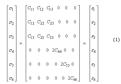
1.3.2 Review of Equations

Wood materials are commonly assumed to be orthotropic because they possess different properties in three directions―longitudinal, tangential, and radial. The elastic stiffness of an orthotropic material is characterized by nine independent constants. The nine elastic constants are E₁₁, E₂₂, E₃₃, G₁₂, G₁₃, G₂₃, v₁₂, v₁₃, and v₂₃, where E = Young’s modulus, G = shear modulus, and v = Poisson’s ratio.

The general constitutive relationship for an orthotropic material, written in terms of the principal material directions⁽¹⁶⁾ is:

Subscripts 1, 2, and 3 refer to the longitudinal, tangential, and radial stresses and strains (s₁ = s₁₁, s₂ = s₂₂, s₃ = s₃₃, e₁ = e₁₁, e₂ = e₂₂, and e₃ = e₃₃, respectively). Subscripts 4, 5, and 6 are a shorthand notation that refers to the shearing stresses and strains (s₄ = s₁₂, s₅ = s₂₃, s₆ = s₁₃, e₄ = e₁₂, e₅ = e₂₃, and e₆ = e₁₃). As an alternative notation for wood, it is common to substitute L (longitudinal) for 1, R (radial) for 2, and T (tangential) for 3. The components of the constitutive matrix, C_ij, are listed here in terms of the nine independent elastic constants of an orthotropic material:

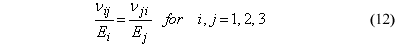
The following identity, relating the dependent (minor Poisson’s ratios v₂₁, v₃₁, and v₃₂) and independent elastic constants, is obtained from symmetry considerations of the constitutive matrix:

Another common assumption is that wood materials are transversely isotropic. This means that the properties in the tangential and radial directions are modeled the same (i.e., E₂₂ = E₃₃, G₁₂ = G₁₃, and v₁₂ = v₁₃). This reduces the number of independent elastic constants to five: E₁₁, E₂₂, v₁₂, G₁₂, and G₂₃. Furthermore, the Poisson’s ratio in the isotropic plane, v₂₃, is not an independent quantity. It is calculated from the isotropic relationship v  = (E – 2G)/2G, where E = E₂₂ = E₃₃ and G = G₂₃. Transverse isotropy is a reasonable assumption if the difference between the tangential and radial properties is small in comparison with the difference between the tangential and longitudinal properties.

The wood model formulation is transversely isotropic because the clear wood data in table 1 for southern yellow pine do not distinguish between the tangential and radial moduli. In addition, the clear wood data for Douglas fir in table 2 indicate that the difference between the tangential and radial moduli is less than 2 percent of the longitudinal modulus.

1.3.3 Default Elastic Stiffness Properties

Room-temperature moduli at saturation (23-percent moisture content) are listed in table 3. The same stiffnesses are used for graded wood as for clear wood. For southern yellow pine, the default Young’s moduli are average tensile values obtained from empirical fits to the clear wood data given in table 1 and shown in appendix B. These fits were published by FPL.⁽¹³⁾ For Douglas fir, the default Young’s moduli and Poisson’s ratios are also obtained from empirical fits, made by the contractor, to the clear wood data given in table 2. The shear moduli were not measured. For both wood species, the parallel shear modulus is estimated from predicted elastic parameter tables for softwoods found in Bodig and Jayne.⁽¹⁶⁾ The perpendicular shear modulus, G₂₃, is calculated from the isotopic relationship between G₂₃, E₂₂, and v₂₃. For both wood species, the value of the perpendicular Poisson’s ratio used to estimate G₂₃ is that measured for Douglas fir (because no values are listed in table 1 for pine).

1.3.4 Orientation Vectors

Because the wood model is transversely isotropic, the orientation of the wood specimen must be set relative to the global coordinate system of LS-DYNA. The transversely isotropic constitutive relationships of the wood material are developed in the material coordinate system (i.e., the parallel and perpendicular directions). The user must define the orientation of the material coordinate system with respect to the global coordinate system. Appropriate coordinate transformations are formulated in LS-DYNA between the material and global coordinate systems. Such coordinate transformations are necessary because any differences between the grain axis and the structure axis can have a great effect on the structural response.

Keep in mind that the wood grain axis may not always be perfectly aligned with the wood post axis because trees do not always grow straight. It is up to the analyst to set the alignment of the grain relative to the wood post in LS-DYNA simulations.

Previous | Table of Contents | Next