U.S. Department of Transportation
Federal Highway Administration
1200 New Jersey Avenue, SE
Washington, DC 20590
202-366-4000
Federal Highway Administration Research and Technology
Coordinating, Developing, and Delivering Highway Transportation Innovations
 |
| This report is an archived publication and may contain dated technical, contact, and link information |
|
Publication Number: FHWA-HRT-04-097
Date: August 2007 |
||||||||||||||||||||||||||||||||||||||||||||||||||||||||||||||||||||||||||||||||||||||||||||||||||||||||||||||||||||
Measured Variability Of Southern Yellow Pine - Manual for LS-DYNA Wood Material Model 143PDF Version (2.92 MB)
PDF files can be viewed with the Acrobat® Reader® 1.7 POSTPEAK SOFTENINGIn addition to predicting the critical combination of stresses at failure, modeling post-failure degradation of these stresses (softening) is particularly important. Postpeak degradation occurs in the tensile and shear modes of wood. This was previously demonstrated in figure 3. 1.7.1 Degradation ModelDegradation models are used to simulate postpeak softening. A choice was made between simple and sophisticated approaches for modeling degradation. Simple degradation models fit into one of three categories: instantaneous unloading, gradual unloading, and no unloading (constant stress after yielding, as modeled with plasticity). Although tensile and parallel shear failures are brittle, instantaneous unloading over one time step would cause dynamic instabilities. An alternative is to gradually unload over a number of time steps. Although simple to implement, such an ad hoc treatment will produce mesh-size dependency. This means that the same physical problem will produce different results for different mesh configurations. Two other disadvantages of these formulations are: (1) stiffness is not degraded in conjunction with strength and (2) progressive softening is independent of subsequent loading. Both of these behaviors are unrealistic. A more sophisticated approach is to model degradation with a damage formulation. A scalar damage parameter, d, transforms the stress tensor associated with the undamaged state,
The stress tensor Damage Parameter Functional Form Two damage formulations are implemented for modeling degradation of wood: one formulation for the parallel modes and a separate model for the perpendicular modes: Parallel Modes
Perpendicular Modes
For each formulation, damage is specified by three user-supplied parameters. For the parallel modes, these parameters are A,B, and The evolution of the damage parameter d is shown in figure 15 as a function of t. The strain-based energy term t is calculated by the model. Its analytical form for both the parallel and perpendicular modes is discussed in subsequent paragraphs. Damage accumulates when t exceeds an initial damage threshold t0. Four curves are shown in figure 15 that correspond to four sets of softening parameters, C and D. The parameter C sets the midslope of the curve near d = 0.5 (larger values of C produce larger midslopes). The parameter D sets the initial slope near the threshold (smaller values of D produce larger initial slopes). Here, t0 » 0.055.
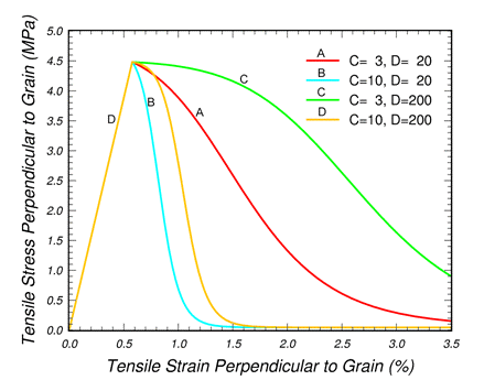
Figure 15. Damage d accumulates with energy t once an initial threshold t0 is exceeded. Softening is demonstrated in figure 16 for tensile failure perpendicular to the grain. Four softening curves are shown, which correspond to the four sets of softening parameters previously used in figure 15. The parameters C and D shape the softening curve. Larger values of D produce a flatter peak. Larger values of C produce more severe softening.
Figure 16. Softening depends on the values of the damage parameters C and D(calculated with dmax = 1). Damage Parameter Strain Basis Damage formulations are typically based on strain, stress, or energy. The wood model bases damage accumulation on the history of strains. One of the more famous strain-based theories is that proposed by Simo and Ju for modeling damage in isotropic materials such as concrete.(21) They base damage on the total strains and the undamaged elastic moduli. They do this by forming the undamaged elastic strain energy norm,
2 The stress tensor Separate strain energy norms are implemented for modeling damage accumulation in the parallel and perpendicular modes. Parallel Modes Damage in the parallel modes is based on the following strain energy norm:
Wood is being treated as transversely isotropic; therefore, t|| was chosen to be the portion of the undamaged elastic strain energy that is associated with the parallel modes (specific terms from equation 51 were retained that contain the parallel normal and shear strains). Damage accumulates when t|| exceeds Perpendicular Modes Damage in the perpendicular modes is based on the following strain energy norm:
The term t^ was chosen to be the portion of the undamaged elastic strain energy that is associated with the perpendicular modes (specific terms from equation 51 are retained that contain the perpendicular normal and shear strains). Damage accumulates when t^ exceeds Strength Coupling Another issue is strength coupling, in which degradation in one direction affects degradation in another direction. If failure occurs in the parallel modes, then all six stress components are degraded uniformly. This is because parallel failure is catastrophic and will render the wood useless. The wood is not expected to carry load in either the parallel or perpendicular directions once the wood fibers are broken. If failure occurs in the perpendicular modes, then only the perpendicular stress components are degraded. This is because perpendicular failure is not catastrophic (the wood is expected to continue to carry the load in the parallel direction). Based on these assumptions, the following degradation model is implemented:
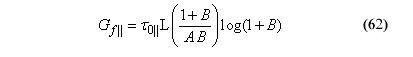
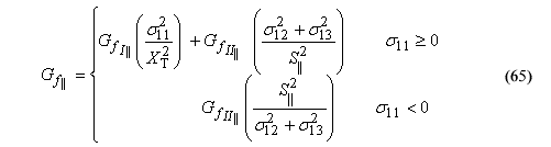
1.7.2 Regulating Mesh-Size DependencyIf a model is mesh-size dependent, then different mesh refinements produce different computational results. This is undesirable and is the result of modeling element-to-element variation in the fracture energy instead of modeling uniform fracture energy. Fracture energy is the area under the stress-displacement curve in the softening regime. If the fracture energy is not constant from element to element, then excess damage will accumulate in the smallest elements because the fracture energy is less in the smaller elements. Regulatory methods eliminate this variation and the excess damage accumulation. Fracture energy is a property of a material and special care must be taken to treat it as such. There are a number of approaches for regulating mesh-size dependency. One approach is to manually adjust the damage parameters as a function of element size to keep the fracture energy constant. However, this approach is not practical because the user would have to input different sets of damage parameters for each size element. A more automated approach is to include an element-length scale in the model. This is done by passing the element size through to the wood material model and internally calculating the damage parameters as a function of element size. Finally, viscous methods for modeling rate effects also regulate mesh-size dependency. However, if rate-independent calculations are performed, then viscous methods will be ineffective. The wood model regulates mesh-size dependency by explicitly including the element size in the model. The element size is calculated as the cube root of the element volume. Softening in the parallel and perpendicular modes is regulated separately because different fracture energies are measured in the parallel and perpendicular modes. Parallel Mode Regularization The relationship between the parallel fracture energy, Gf||; the softening parameters, A and B; and the element size, L, is:
This expression for the fracture energy was derived by integrating the analytical stress-displacement curve:
where:
The fracture energy varies with failure mode in the following manner:
When failure is entirely tensile (s11 = XT, s12 = s13 = 0), then piecewise function of tension fracture energy and softening is brittle. When failure is entirely shear Perpendicular Mode Regularization An expression similar to equation 62 is readily obtained for the fracture energy perpendicular to the grain:
To regulate mesh-size dependency, the wood model requires input values for D, When the perpendicular failure criterion is satisfied, the wood material model internally solves equation 66 for the value of C based on the initial element size, initial damage threshold, and fracture energy for the particular mode of perpendicular failure that is initiated (tensile, shear, or compressive):
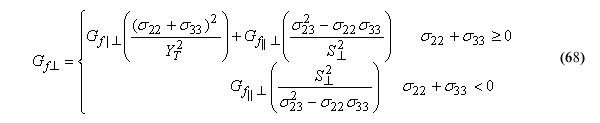
Fracture energy varies with failure mode in the following manner:
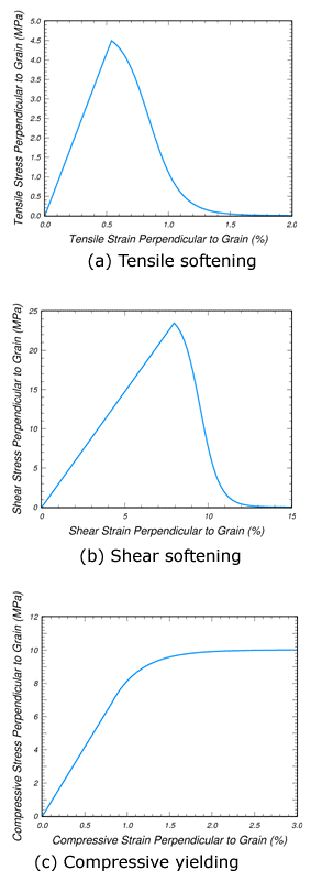
When failure is entirely tensile (s22 + s33 = YT, s23 = 0), then Stress-strain curves for these failure modes are given in figure 18. They were calculated for the default moduli, strengths, and fracture energies at 12-percent moisture content.
Figure 17. Softening response modeled for parallel modes of southern yellow pine.
Figure 18. Softening response modeled for perpendicular modes of southern yellow pine. 1.7.3 Default Damage ParametersThe damage model requires input of eight damage parameters―four for the parallel modes (B,
Fracture energies for Douglas fir are set equal to those for southern yellow pine. This is because fracture intensity data are not available for Douglas fir, and grade 1 bogie-post impact simulations correlated with test data suggest that this assumption is reasonable.(2) Measured Fracture Intensities The effect of moisture content on the mode I and mode II fracture intensities of southern yellow pine is given in table 9 for the perpendicular modes. These data were measured with the load applied in the tangential direction and the crack propagation in the longitudinal direction.(13) Fracture intensities were measured from compact-tension specimens (7.62 by 8.26 by 2.0 cm) and center-split beams (65 by 6 by 2 cm). No data are reported for the parallel modes. Published data indicate that the mode I fracture intensities measured parallel to the grain are about seven times those measured perpendicular to the grain.3(16)3 Personal communication with Dr. David Kretschmann of FPL.
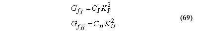
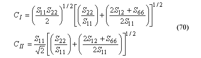
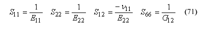
Derived Fracture Energies The mode I and mode II fracture energies are related to the fracture intensities through the following analytical expressions:
where:
Here, the compliance coefficients, Sij, are the reciprocals of the elastic moduli:
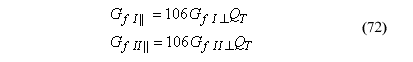
The values of C| and C|| vary with moisture content because moduli vary with moisture content (see appendix B). Tensile and shear perpendicular fracture energies as a function of moisture content are derived from equation 69 and FPL’s quadratic equations for fracture intensity as a function of moisture content. Default fracture energies at saturation are given in table 10 for the perpendicular modes of pine and fir. These values are default values regardless of the grade or temperature of the wood. No fracture intensity or energy data are available for the parallel modes, so default values are based on LS-DYNA bogie-post impact simulations correlated with test data.(2) Correlations were made for grade 1 pine and fir posts, DS-65 pine posts, and frozen grade 1 pine posts. Good room-temperature grade 1 correlations (pine and fir) are obtained when the fracture energy parallel to the grain is 50 times greater than the fracture energy perpendicular to the grain. This parallel-to-perpendicular factor of 50 for energy is consistent with a parallel-to-perpendicular factor of 7 for intensity once equation 69 is applied (72 » 50).(16) In addition, good DS-65 correlations are obtained with a factor of 85, which indicates that the parallel fracture energy depends on the grade. To accommodate variation with grade, the default parallel-to-the-grain fracture energies are modeled as:
These equations indicate that the default fracture energy of clear wood, parallel to the grain, is 106 times greater than the default fracture energy perpendicular to the grain. Default fracture energies derived from the above equations are given in table 10 for the parallel modes of pine and fir. 1.7.4 Modeling BreakawayComplete failure and breakup of a wood post is simulated with element erosion.4 The erosion location is determined by the wood model from the physics of the problem. Dynamic instability is not an issue because the element erodes after it loses all strength and stiffness. In addition, mesh-size sensitivity is regulated through the damage formulation. Parallel damage is catastrophic because cracking occurs across the grain, which breaks the fibers or tubular cells of the wood. An element will automatically erode if it fails in the parallel mode and the parallel damage parameter exceeds d|| = 0.99. Recall that default dmax|| = 0.9999, so the element erodes just prior to accumulating maximum damage. All six stress components are degraded with parallel damage, so the element loses nearly all strength and stiffness before eroding. If the user sets dmax|| < 0.99, then erosion will not occur. Perpendicular damage is not catastrophic because cracking occurs between the fibers, causing the wood to split at relatively low strength and energy levels. The fibers are not broken. An element does not automatically erode if it fails in the perpendicular mode. This is because only three (sR, sT, and sRT) of the six stress components are degraded with perpendicular damage. Since erosion does not automatically occur, dmax^ is set to 0.99 instead of 0.9999 so that the element retains 1 percent of its elastic stiffness and strength. In this way, computational difficulties associated with extremely low stiffness and strength will hopefully be avoided. As an option, a flag is available, which, when set, allows elements to erode when the perpendicular damage parameter exceeds d^ = 0.989. Setting this flag is not recommended unless excessive perpendicular damage is causing computational difficulties. As an additional precaution, an element will erode if d^ > 0.98, and the perpendicular normal and shear strains exceed a predefined value of 90 percent. Typically, erosion is more computationally efficient than the alternative approach of modeling fracture surfaces using tied surfaces with failure. One drawback of the tied surface approach is that an interface model (criteria) must be developed and validated for the tied nodes because the wood model is for elements, not interfaces. Another drawback is that the user must mesh the entire model with tied interfaces or else guess the failure location prior to running the calculation in order to specify the tied surface location. This is not practical. Other drawbacks are dynamic instability caused by sudden tied-node failure and mesh-size sensitivity. |
||||||||||||||||||||||||||||||||||||||||||||||||||||||||||||||||||||||||||||||||||||||||||||||||||||||||||||||||||||


 , into the stress tensor associated with the damaged state,
 . For the perpendicular modes, these parameters are C,D, and
  . The parameter
  limits the maximum level of damage. It ranges between 0 and 1. No damage accumulates if
  =0. Typically,
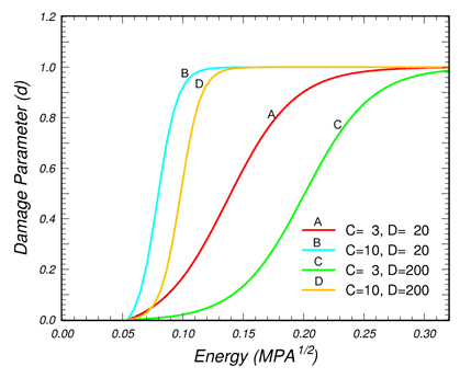
 . For simplicity,
  where Cijkl is the linear elasticity tensor previously given in equation 1. One way of expanding
 is not equal to the elasto-viscoplastic stress tensor
  . It is a fictitious stress that is based on the total strain and is defined for convenience.
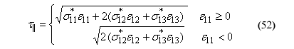
 . The initial threshold
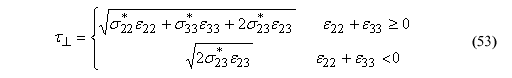
 . The initial threshold


 . In addition, the functional form of d is given by equation 49 with dmax = 1.
 , rather than A and B. When the parallel failure criterion is satisfied, the wood material model internally solves equation 62 for the value of A based on the initial element size, initial damage threshold, and fracture energy for the particular mode of parallel failure that is initiated (tensile, shear, or compressive):
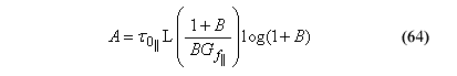
 , then
  and softening is more gradual. When failure is compressive (
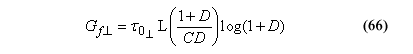
 , and
, and  , rather than C and D.
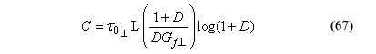
 and softening is brittle. When failure is entirely shear
  , then
  and softening is more gradual. When failure is compressive
  , then Gf =
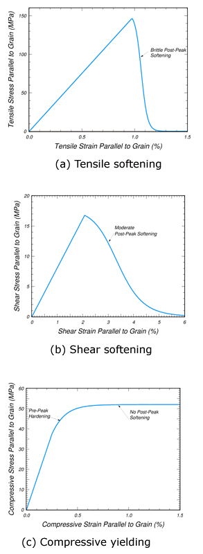
 ,
,  ,
,  , and dmax