U.S. Department of Transportation
Federal Highway Administration
1200 New Jersey Avenue, SE
Washington, DC 20590
202-366-4000
Federal Highway Administration Research and Technology
Coordinating, Developing, and Delivering Highway Transportation Innovations
 |
| This report is an archived publication and may contain dated technical, contact, and link information |
|
Publication Number: FHWA-HRT-08-051
Date: June 2008 |
|||||||||||||||||||||||||||||||||||||||||||||||||||||||||||||||||||||||||||||||||||||||||||||||||||||||||||||||||||||||||||||||||||||||||||||||||||||||||||||||||||||||||||||||||||||||||||||||||||||||||||||||||||||||||||||||||||||||||||||||||||||||||||||||||||||||||||||||||||||||||||||||||||||||||||||||||||||||||||||||||||||||||||||||||||||||||||||||||||||||||||||||||||||||||||||||||||||||||||||||||||||||||||||||||||||||||||||||||||||||||||||||||||||||||||||||||||||||||||||||||||||||||||||||||||||||||||||||||||||||||
Surrogate Safety Assessment Model and Validation: Final ReportPDF Version (3.39 MB)
PDF files can be viewed with the Acrobat® Reader® Chapter 4. Field ValidationThis chapter presents the field validation effort, wherein 83 field sites—all four-leg, signalized intersections—were assessed with SSAM, and the results were compared to actual crash histories. This contributes to a three-part overall validation effort consisting of the following:
In the preceding chapter, the theoretical validation effort assessed the use of SSAM to discern the relative safety of pairs of intersection/interchange design alternatives in a series of 11 case studies. The field validation in this chapter concerns the direct accuracy of surrogate safety estimates for a signalized, four-leg intersection, which is measured by correlation to actual crash frequencies. This also affords a comparison of surrogate safety estimates with traditional ADT-based models for crash prediction. The validation testing in this chapter is based solely on modeling with the VISSIM simulation. The next chapter completes the validation effort, using SSAM to reassess 5 intersections (of the 83 considered in the field validation) with each of 4 simulation systems: AIMSUN, Paramics, TEXAS, and VISSIM. That effort will characterize the sensitivity and/or bias of the surrogate safety measures as they differ when obtained from each of the four simulations. This chapter is organized into the following sections:
PURPOSEThe main purpose of the field validation effort is to compare the predictive safety performance capabilities of the SSAM approach with actual crash experience at North American signalized intersections. This effort consists of a series of statistical tests to assess the correlation between actual crash frequencies at a series of intersections and the corresponding frequency of conflicts observed in simulation models of these intersections. Traditional volume-based crash prediction models are used as a basis for comparison. Ideally, SSAM would reveal a more accurate picture of safety than the ADT of intersection crossroads. However, given that SSAM can yield safety assessments over a much more flexible range of traffic facilities than traditional crash prediction models, including simulated designs that have never been built, the standard of better performance than traditional models is not a fundamental requirement for utility. METHODOLOGYThe methodology used in the field validation task is based on relating actual crash data from real-world intersections with the corresponding surrogate safety measures that SSAM derives from simulation models of those same intersections. Throughout this discussion, the term incidents will be used in a more abstract sense to refer to either crashes or conflicts. As mentioned previously, the field validation effort entailed the analysis of 83 intersections, modeled with the VISSIM simulation. Selection of the 83 filed sites and VISSIM modeling issues are discussed in subsequent sections. This section introduces a series of five statistical tests used in this validation effort:
Test 1: Intersection Ranking by Total IncidentsIn this test, the ranking of intersections from SSAM according to average conflict frequency is compared to the ranking of the same intersections using actual crash frequency. This test consists of the following three steps (A, B, and C): Step A: Conflict Ranking In this step, the average hourly conflict frequency found by SSAM is used as the expected total number of conflicts at each intersection. Each intersection was simulated for five replications, each lasting 1 hour. Thus, the sum of all conflicts recorded over all five replications will be divided by 5 to determine the average hourly conflict frequency in terms of conflicts per hour. In this validation test, the intersections will be ranked based on their average hourly conflict frequency in descending order. Step B: Crash Ranking In this step, the average yearly crash frequency for each intersection is determined by dividing the total number of crashes over the observation period by the number of years in the observation period. At least 3 years of crash data are available for all intersections in the study, though some intersections have more data. The intersections are then ranked based on their average yearly crash frequency in descending order. Step C: Ranking Comparison The intersection rankings based on average hourly conflict frequency will be compared to the intersection rankings based on average yearly crash frequency. The Spearman rank correlation coefficient can be used to determine the level of agreement between the two rankings. The Spearman rank correlation coefficient is often used as a nonparametric alternative to a traditional coefficient of correlation and can be applied under general conditions. The Spearman rank correlation coefficient (ρs) is calculated as shown in figure 114. [6] A score of 1.0 represents perfect correlation and a score of 0 indicates no correlation. An advantage of using (ρs) is that when testing for correlation between two sets of data, it is not necessary to make assumptions about the nature of the populations sampled.
Figure 114. Equation. Spearman Rank Correlation Coefficient. Where: di is the difference between two rankings for item i. n is the number of items ranked. Under a null hypothesis of no correlation, the ordered data pairs are randomly matched, and thus, the sampling distribution of (ρs) has a mean of 0 and the standard deviation (
Figure 115. Equation. Standard Deviation for Paired Data Samples. Because this sampling distribution can be approximated with a normal distribution even for relatively small values of n, it is possible to test the null hypothesis on the statistic given in figure 115. This value can be compared to a critical z-value. For this analysis, a z-value of 1.64 is selected, representing a 90-percent level of significance, or a z-value of 1.96 for a 95-percent level of significance. Significance levels of 90 percent and 95 percent would be satisfied by the Spearman coefficient (ρs) values in excess of 0.18 and 0.22, respectively.
Figure 116. Equation. Critical Z-Value. Test 2: Intersection Ranking by Incident TypesTest 2 repeats the same comparative ranking procedures as test 1, but for subsets of specific incident (i.e., crash/conflict) types. For example, the analysis can be repeated for the following types:
SSAM classifies all conflicts amongst these three types and provides counts for each type. The average hourly conflict frequency for each conflict type is computed as in test 1, and these results are used to rank the intersections for each conflict type. To provide type-specific crash frequencies, all crash reports from Insurance Corporation of British Columbia (ICBC) were reviewed to determine whether it was a rear-end incident, crossing incident, or lane-changing incident. This classification was readily evident in the vast majority of cases. In the few cases where the classification was not obvious, engineering judgment was applied to determine the most representative type. Average yearly crash frequencies were tabulated for each incident type, rank ordered, and compared using the Spearman’s rank correlation test, as in test 1. The results of this step will demonstrate the capability of SSAM to accurately identify and rank intersections that carry a high risk for specific crash types. Test 3: Conflicts-Based Crash-Prediction Regression ModelTest 3 will establish the correlation between conflicts and crashes by developing a regression equation to estimate average yearly crash frequencies at an intersection as a function of the average hourly conflict frequencies found by SSAM. Thus, a conflicts-based model for crash-prediction will be developed, and goodness-of-fit testing will be used to determine the strength of the relationship between conflicts and crashes. This test could be conducted using either frequency or rate, although exposure can be excluded due to the paired nature of the test. As a benchmark basis for comparison, a traditional volume-based model for crash prediction will also be developed. The conflicts-based crash-prediction model will then be compared to a volume-based crash-prediction model to gauge the relative capabilities of surrogate safety assessment versus traditional approaches that are primarily driven by traffic volume. Standard generalized linear modeling (GLM) techniques are used to calculate the expected crash frequency at each intersection,(24, 25) using the GENMOD procedure in the SAS® 9.1 statistical software package. Three statistical measures are provided to assess the goodness of fit of the models to the raw crash data for the 83 intersections. The first measure is the Pearson chi-squared computed by the following:
Figure 117. Equation. Pearson Chi-Squared Goodness of Fit Measure. Where: E(Λi) is the predicted crash frequency of intersection i. yi is the actual crash frequency of intersection i. n is the number of intersections. The second statistical measure used for assessing the goodness of fit is the scaled deviance. This is the likelihood ratio test statistic measuring twice the difference between the log-likelihood of the data under the developed model and its log-likelihood under the full (“saturated” model). The scaled deviance is computed by the following:
Figure 118. Equation. Scaled Deviance Measure. There are several approaches to estimate the shape parameter k of the negative binomial distribution with the method of maximum likelihood being the most widely used. The method of maximum likelihood will be used in this analysis. The third goodness-of-fit measure is the R-squared defined by Miaou.(26) The R-squared goodness of fit test is computed as:
Figure 119. Equation. R-Squared Goodness of Fit Measure. Where:
Test 4: Identification of Incident-Prone Locations.The following fours steps (A, B, C, and D) will be conducted for this test: Step A A conflict prediction model will be developed (using standard GLM procedures) to predict intersection conflicts frequency (the data calculated by SSAM) as a function of the intersection traffic volume. Step B A crash prediction model will be developed (using standard GLM procedures) to predict intersection crash frequency (the actual crash data) as a function of the intersection traffic volume. Step C The two prediction models will be compared to determine whether or not the conflict prediction model can predict risk in a manner similar to the crash prediction model for intersections with the same characteristics. This comparison consists of identification and ranking of crash/conflict prone locations. A crash/conflict prone location is defined as any location that exhibits a significantly higher number of crashes/conflicts as compared to a specific, so-called “normal” value. The Empirical Bayes (EB) technique improves the location-specific prediction and thus is used to identify hazardous locations. The EB refinement method identifies problem sites according to the following four-step process:
Once crash/conflict-prone sites are identified, it is important to rank the locations in terms of priority for treatment. Ranking problem sites enables the road authority to establish an effective road safety program, ensuring the efficient use of the limited funding available for road safety. Sayed and Rodriguez suggest using one of two techniques that reflect different priority objectives for a road authority. (25) The first ranking criterion is to calculate the ratio between the EB estimate and the predicted frequency as obtained from the GLM model (a risk-minimization objective). The ratio represents the level of deviation that the intersection is away from a “normal” safety performance value, with the higher ratio representing a more hazardous location. The second criterion, the cost-effectiveness objective, is a “potential for improvement” (PFI) criterion, which is calculated as the difference between the observed crash/conflict frequency and the volume-based estimate of “normal” crash/conflict frequency. Step D Two comparisons will be undertaken. The first is to compare the locations identified as crash-prone to intersections identified as conflict-prone. The second is a comparison of both the “risk ratio” and PFI intersection rankings obtained using crash data to the corresponding rankings obtained using conflict data. Test 5: Identification of Type-Specific Incident-Prone LocationsTest 5 will repeat the same comparative analysis as test 4 for the following subsets of crash/conflict types:
FIELD DATAGuidelines for the selection of signalized intersections for the field validation included the following:
Based on these guidelines, 83 signalized intersections, all with four-leg geometry, were selected from a much larger database of Canadian intersections. The information was collected from safety studies performed by Hamilton Associates of Vancouver, BC. The following data were available for each intersection:
Crash records were assembled from the auto insurance claims data files collected by the ICBC. The auto insurance claims data maintained by ICBC are current and comprehensive and are considered reliable for intersections in British Columbia.(28) Appendix A provides a summary of the 83 intersections used in this study. The appendix shows, for each intersection, the cross street names, number of lanes on each approach, the angle of skew (or at least which approaches are skewed), the signal control type, average daily traffic (ADT) for the major and minor roads, and the AM peak-hour volumes. It is evident from summary descriptions provided in appendix A that although all 83 intersections were four-leg signalized, they still represent a wide range of traffic characteristics. SIMULATION MODELING OF FIELD SITESThe 83 intersections used in this study were coded in VISSIM simulation system. This selection was based on VISSIM’s flexibility to model complex geometric configurations and ability to provide the user with control over operational/driver behavior parameters. Throughout the validation effort, the team iteratively upgraded from VISSIM version 4.0, to versions 4.1 and then 4.2 to take advantage of enhancements, some of which were motivated by preliminary findings of the SSAM validation effort. Modeling ProcessThe process of modeling a single intersection in VISSIM starts by tracing an aerial photo of the intersection, specifying each approach number, width, and length of lanes. Once the geometry of the intersection is defined, traffic flows (i.e., vehicles per hour) for each approach are allocated for all directions. Morning peak-hour volumes were utilized for this study. The next step is to encode the signal control parameters. The NEMA-style controller model included with VISSIM was used for all intersections in this study. Detector locations were defined for intersections with full- or semi- actuated control strategies. [7] Key modeling features of VISSIM related to the evaluation of surrogate safety measures are the implementation of priority rules for permissive left-turn and right-turn-on-red (RTOR) maneuvers and the modeling of reduced-speed areas for turning movements. The inclusion of reduced-speed areas is important not only for realistic modeling of traffic, but it also impacts the measurements of yield points for priority rules. The effects of priority-rule modeling on the surrogate measures of safety outputs from the simulation system are be discussed in subsequent sections. Finally, speed profiles, vehicle-type characteristics, and traffic composition parameters are configured for each intersection. Each intersection was modeled in VISSIM and tested for realistic and reasonable vehicle behaviors. After this nominal verification, the intersection was simulated five times for a period of 1 hour with different random seed values. Once the VISSIM runs were completed, the TRJ output files from VISSIM were imported into the SSAM application to identify traffic conflicts and calculate corresponding surrogate safety measures. VISSIM AssumptionsSome assumptions had to be made pertaining to intersection geometry, signal control, speed profiles, vehicle type characteristics, traffic compositions, and priority rules. These assumptions are described in the following subsections. Intersection Geometry Only 19 intersections had aerial photos on file. The other 64 intersections were based on schematic photos showing some dimensions and certain provisions were made to trace these intersections into VISSIM. For all 83 intersections, no information was provided on the number or size of the departing traffic lanes. In some cases, this information can be estimated from the aerial photos; in other cases, assumptions had to be made. Signal Control and Detectors The simulated intersections included both pre-timed and actuated signal control. Several assumptions were made when modeling the actuated signalized intersections. In cases where a signal has actuated protected/permitted left turning phases, the opposing left turning phases were linked together in order to start and end at the same time. No information on detector locations was available from the safety studies files. Therefore, the detectors were assumed to have a length of 3 m (9.28 ft) and were placed 5 (15.28 ft) m before the stop line. Both assumptions are based on the “standard practice” employed in the province of British Columbia. Speed Profiles, Vehicle Type Characteristics & Traffic Compositions The traffic composition was assumed to be entirely composed of passenger cars. The desired speed profile was assumed to range from 50 to 65 km/h (31.05 to 40.365 mi/h). Since no information was provided on the percentage of trucks present in each intersection, none were included in the analysis, as the standard practice in British Columbia restricts heavy trucks from using main arterial roads during peak hours. Using VISSIM version 4.0-12, SSAM found an excessive number of lane-change conflicts, as explained in detail later in this chapter. Many of these conflicts occurred during partially complete lane changes where a vehicle slow or stopped at an angle while changing lanes, and trailing vehicles drove right through the tail of this vehicle. Modifications were made to VISSIM and included in versions 4.0-15 and 4.1, introducing new vehicle type codes (or classes) greater than 1 million and greater than 2 million. With types greater than 1 million, the vehicles were modeled as always driving parallel to the travel lane when changing lanes, rather than tilted as before. This reduced the drive-through conflicts, but increased rear-end conflicts when changing into destination lanes with a closely trailing vehicle. Vehicles with a type value greater than 2 million also travel parallel to the link during lane changes and refrain from starting a lane change unless the gap in front of the trailing vehicle in the new lane is sufficient to perform the maneuver, thereby reducing rear-end conflicts with that vehicle. Priority Rules A priority rule in VISSIM is the mechanism with which the user can define the yielding and gap-acceptance behavior of vehicles in the simulation. A priority rule is defined through three parameters: minimum gap size, minimum headway, and maximum speed. The VISSIM 4.1-12 user manual suggests defining priority rules for only permissive left turns and right turns on red, although in certain geometric situations it is necessary to add priority rules to be consistent with real driving behavior.(29) In general, for free-flow traffic on the main road, the minimum gap time of the priority rule is the most relevant condition to calibrate the performance of crossing vehicles. For slow moving or queuing traffic on the main road, the minimum headway becomes the most relevant parameter in calibrating the priority rule. The default parameters as suggested by PTV for minimum gap, minimum headway, and maximum speed are 3 seconds, 5 m (15.28 ft), and 180 km/h (112 mi/h), respectively. For the 83 intersections used in this study, a minimum gap of 3 seconds resulted in a large number of simulated crashes. Therefore, the minimum gap size was increased to 5 seconds with an additional 0.5 seconds for any additional crossing lane. More discussion on the effect of varying the minimum gap size is presented in a validation issues section later in this chapter. To be consistent with real-life behavior, additional priority rules were added for exclusive left-turn and right-turn bays. For intersections with no exclusive left-turn and right-turn bays, priority rules were defined to eliminate run-over crashes between through-movement vehicles, right-turn vehicles, and vehicles waiting for a left turn in the middle of the intersection. More discussion on the effect of changing the parameters and the introduction or removal of priority rules are presented in a validation issues section later in this chapter. Miscellaneous Assumptions No on-street parking information was available in the safety studies data; therefore, this behavior was not modeled. It is a standard practice in the province of British Columbia to prohibit on-street parking during peak hours, thus justifying this assumption. Furthermore, no pedestrian volumes were available; therefore, pedestrians’ behavior and interaction were not accounted for in the analysis. Car-following and lane-changing behavior were set to model urban (motorized) traffic flow using the Wiedemann 74 model with all default parameters used.(29) All traffic flows input to VISSIM were based on AM peak volumes, as recorded in the safety studies database for each intersection. The AM volumes used for simulation are included in table 122 in appendix A. Modeling IssuesModeling Schemes This section describes the inputs of two modeling schemes developed in conjunction with PTV referred to as:
Scheme 1 consists of 16 priority rules, in addition to the modeling assumptions mentioned previously. There are 8 priority rules governing permissive-left and RTOR maneuvers, and there are 8 priority rules governing exclusive left-turn and right-turn bays. Scheme 1 was adopted in early analysis and certain refinements were proposed.
Scheme 2, which has 32 priority rules defined, builds on the initial 16 priority rules defined for Scheme 1 and includes an additional 16 rules to compensate for inappropriate behavior during yellow and red clearance intervals. This inappropriate behavior was observed in several situations where the signal state turned from green to yellow and then red with a left-turning vehicle waiting to perform its turning maneuver in the middle of the intersection. During the yellow and red clearance intervals, the vehicles within the intersection were run over by opposing traffic. In real-life behavior, opposing through or other left-turning vehicles will wait for traffic to clear before proceeding into the intersection. The additional 16 priority rules in Scheme 2 were designed to allow for such a behavior. The Scheme 2 rules were adopted for reanalysis of 83 intersections. To demonstrate the effect of redefining the priority rules on SSAM output, a comparison between the SSAM results for the two modeling schemes is presented later in this chapter. In addition to the aforementioned rules, the follow changes were made before a final reanalysis of the 83 intersections:
Simulated Crashes Despite all the modeling techniques that were employed, simulated crashes remained in the model. These crashes result from insufficient minimum gap size, a vehicle’s failure to yield to a priority rule, or as a result of an abrupt lane change of a vehicle in an intersection or during queuing. All necessary precautions were taken to minimize the number of simulated crashes while maintaining a level of consistency in modeling all intersections. Therefore, certain parameters were adjusted to reduce the number of simulated crashes experienced in VISSIM. As a result, the number of simulated crashes recorded at each intersection was decreased considerably. However, simulated crashes continued to occur, specifically for intersections with high volumes. These intersections experienced a large number of simulated crashes due to the abrupt lane-changing behavior, described in detail in the following subsection. Preliminary analysis with SSAM was conducted with and without simulated crash data to determine if these simulated crash events should be excluded from the analysis. As in the theoretical validation of the previous chapter, it was decided to exclude simulated crashes from the conflict analysis. Lane-Changing Behavior A large number of conflicts/simulated crashes were observed during this study as the number of cars queued up waiting to perform a right or left maneuver increased. These conflicts/simulated crashes were often recorded by SSAM as either rear-end or lane-changing maneuvers. While an increase in rear-end conflicts was expected with an increase in vehicle stops, this increase in simulated crashes was due to queued cars changing lanes abruptly. It was also expected that as queues increase in shared-movement (through and turning) lanes, and through-moving vehicles were impeded, there would be an increase in lane-changes to circumvent the queue. However, visual inspection of the lane-changing behavior in this particular situation revealed conspicuous misbehavior (e.g., a trailing vehicle simple drives through a vehicle that was stopped midway through a lane-change). It should be noted that this abrupt lane-changing behavior continued to occur in situations where there was no heavy traffic or amongst through-traveling vehicles queuing up at a red signal. Appendix B provides a sequence of screenshots from the simulation animation during a representative example of this lane-changing behavior. At this time, there is no clear justification for the unusual lane-changing behavior in VISSIM. The following measures were taken to reduce the effect of such unusual behavior:
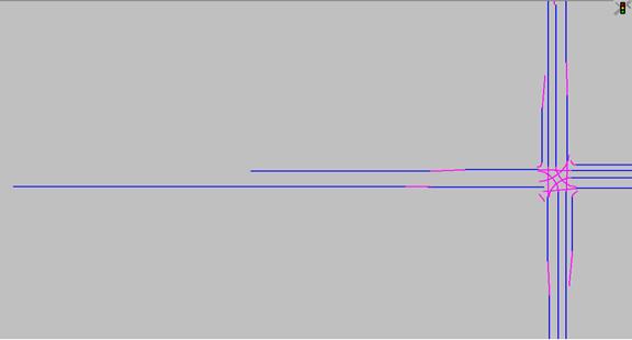
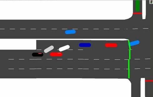
Modeling Left-/Right-Turn Bay Tapers Generally, left- and right-turn bay tapers can be modeled in different ways in VISSIM. Therefore, two configurations were proposed to simulate vehicle movements for exclusive left-turn and right-turn bays. The first configuration proposes the use of one through link and one link for each of the left- and right-turn storage bays. The through link is then connected to the left- and right-turn storage bays by a connector, emulating the shared roadway and providing a smooth transition from the through movement to the left or right. During congestion, because the connector may overlap the through lane, a priority rule should be placed on the connector that prohibits vehicles from moving forward due to inadequate space to enter the taper (in VISSIM, vehicles traveling on separate links and connectors are not recognized by other vehicles even though they are traveling in the same direction). Likewise, a priority rule should be placed so that vehicles queued on the connector are recognized by the through vehicles on the link. This modeling configuration is demonstrated in figure 127, where blue lines indicate links while pink lines indicate connectors. The second modeling configuration proposes the use of two links and a connector between them. The first link will have as many lanes as the through movement requires. The second link will group the left, through, and right lanes with the connector joining the through movements of both links. This configuration will allow vehicles to respond to the internal lane-changing logic to yield to conflicting vehicles for the through, left, and right turn movements. Figure 128 demonstrates this modeling configuration. However, the second configuration has led to a number of problems. Figure 129 s hows how the second configuration resulted in an increasingly high number of conflicts with vehicles not queuing up normally. Therefore, the first configuration was used to model all left- and right-turn tapers.
Figure 127. Screen Capture. First Taper Modeling Configuration.
Figure 128. Screen Capture. Second Taper Modeling Configuration.
Figure 129. Screen Capture. Queuing Problem Due to the Second Taper Configuration. VISSIM Modeling SummaryThe section presented the modeling process and some key modeling assumptions in VISSIM. Several modeling assumptions were presented including assumptions related to intersection geometry, signal control, detectors, speed profiles, vehicle type characteristics, traffic composition, priority rules, and other aspects. As well, the section discussed a number of important modeling issues. These issues included the modeling schemes, the occurrence of simulated crashes, the abrupt lane-changing behavior experienced, and the modeling of left- and right-turn bay tapers. TEST RESULTS AND DISCUSSIONThis section presents the results of the field validation testing effort, the design of which was described in the preceding sections of this chapter. The experimental procedure, prior to statistical testing, is summarized as follows. A set of 83 intersections, selected from field sites in North America, were modeled in VISSIM. Each intersection model was simulated for five replications for 1 hour of simulated time, each with different random seeds. The corresponding five output files (i.e.,TRJ files) from VISSIM were then imported into SSAM for identification of conflicts and computation of the surrogate measures of safety for each conflict event. SSAM was configured to use its default values conflict identification thresholds. Namely, the (default) TTC and PET values used were 1.5 seconds and 5.0 seconds, respectively. The results of the SSAM analysis consists of the number of total conflicts and the number of conflicts of each type of vehicle-vehicle interaction: crossing, rear end, and lane changing. Average hourly conflict counts for each intersection are provided in appendix C. The crash data used for comparison are provided in appendix A, presented in terms of average yearly crash counts for each intersection, including counts by maneuver type and by severity (fatality, injury, and proper damage only). The crash counts were derived by filtering through all intersection crash records to include only two (or more) vehicle crashes. Thus, single-vehicle crashes, such as run-off-road crashes, fixed-object crashes, and animal-, pedestrian-, or bicycle- related crashes, are excluded. Validation Test 1: Safety RankingTest 1 is a comparison of the ranking of intersections based on average hourly conflict frequency versus the ranking of intersections based on average yearly crash frequency. The Spearman rank correlation coefficient (ρs) value of this ranking comparison was 0.463, which is significant at a 95-percent level of confidence. As a basis of comparison, the intersections were ranked on basis of total ADT values, and this was also compared with the ranking based on average yearly crash frequency. The Spearman rank correlation coefficient (ρs) value of this ranking comparison was 0.788, which is significant at a 95-percent level of confidence. The Spearman rank correlation tests show that a significant correlation was found between intersection rankings based on simulated average hourly conflict frequency and average yearly crash frequency; however, a higher correlation was found with intersection rankings based on average daily traffic volume. It is important to note that the simulated conflict data are based on AM peak-hour volumes and not on ADT volumes. The ratio of ADT to AM peak-hour volume for each intersection is shown in table 122 in appendix A. This table shows that the average ratio of all intersections was 25, with a range spanning from 20 to 51. To quantify this relationship in other terms, a correlation (R-squared) of 0.73 was found in a linear regression between the ADT and AM peak-hour volumes of all intersections. The differences between simulated (AM peak) volumes and ADT volumes likely degrades the correlation between simulated conflict frequencies and actual crash counts, which were accumulated during all hours of the day. Crashes and conflicts were clearly proportional to volume, and thus simulating volumes at 1/20th of the ADT for one intersection and 1/50th of the ADT for another intersection does not seem ideal. However, simulating at 1/24th of the ADT is questionable as well. Traffic flow can exhibit strong directional bias in one direction during the morning, and the opposite direction during the evening. Thus, traffic flows at 1/24th of the total ADT might not capture these directional biases. It would seem that the conflict and crash rates would fluctuate relative to the specific patterns of crossing flows and directional bias throughout the day, particularly at intersections with asymmetrically skewed approaches. It is expected that higher correlations could be obtained if simulated volumes better represented the profile of different directional flows and if all intersections were simulated at volumes in uniform proportion to their corresponding ADT values. Indeed, higher correlations were obtained by scaling each intersection by the ratio of ADT to AM peak-hour flows. However, such a scaling technique might well be subject to scrutiny as well. Rather than provide correlation based on such “corrective” measures, it is simply noted that results of this effort are based on simulation of only the AM peak-hour volumes, which could be inferior to correlations possible with more comprehensive simulation. Validation Test 2: Safety Ranking by Incident TypesValidation test 2 repeats the same comparative ranking procedures as for validation test 1 for the subsets of crash/conflict types: crossing, rear end, and lane changing. There were an inadequate number of crossing conflicts recorded to perform the ranking comparison for crossing type incidents. Table 81 compares the distribution of conflicts and crashes by incident type. There were very few crossing conflicts recorded, while nearly 20 percent of crashes were crossing maneuvers. Note that the simulated crashes (i.e., conflicts with a TTC of 0 seconds) were excluded from the conflict count data, as in the theoretical validation. If simulated crashes are included, the percentage of crossing, rear-end, and lane-change conflicts are 1.7 percent, 91.0 percent, and 7.3 percent, respectively. However, most “crashes” observed during simulation appeared to reflect anomalous behavior in the traffic model and were filtered out. Additionally, the use of a PET threshold of 5.0 seconds may also have contribute to underreporting of crossing conflicts, such as whenever a crossing vehicle abruptly decelerates to abort a maneuver (e.g., left turn or right turn) and does not complete that maneuver until a few more vehicles have passed or perhaps for a whole signal cycle (in any case, more than 5.0 seconds). While PET seems to be an important surrogate safety measure, it is evident (in hindsight) that this measure may be inappropriate for screening out conflict events.
There are significant differences between conflict distributions by type and actual crash distributions by type. The ratios of conflicts-per-hour to crashes-per-year for crossing, rear-end, and lane-change conflicts are 0.01, 2.06, and 0.65, respectively. It seems plausible that conflicts-to-crashes ratios may be lower for more severe incidents and higher for less dangerous incidents. That is, accepting that rear-ends are generally less severe than lane-change and rear-end conflicts, there is an abundance of these “lower risk” conflicts. Conversely, a crossing conflict (such as a left turner colliding with opposing through traffic) might generally be regarded as the most dangerous conflict type, and there are significant fewer conflicts per crash for this incident type. This is an evident trend in the data, though by virtue of being based on simulated conflicts and not real-world conflicts, this potential relationship between conflict frequencies and severity is only a conjecture. The low frequency of crossing conflicts could also be due (in whole or in part) to the efforts of modeling priority rules to reduce simulated crashes. Moving on to the results of the ranking tests, there is a significant correlation between conflicts and crashes when considered by conflict type. The Spearman rank correlation coefficient (ρs) value for the rear-end incident ranking comparison was 0.473, which is significant at a 95-percent level of confidence. Also, the Spearman rank correlation coefficient (ρs) value for lane-change incident ranking comparison was 0.469, which is significant at a 95-percent level of confidence. For comparison, the intersections were ranked on basis of total ADT values, and this was also compared with the rankings based on cross, rear-end, and lane-change crashes. All of these ranking comparisons were significant, with Spearman rank correlation coefficient (ρs) values of 0.499, 0.798, and 0.712 for crossing, rear-end, and lane-change incident types, respectively. Rank correlation testing has shown a significant correlation between rear-end conflicts and rear-end crashes and between lane-change conflicts and lane-change crashes. However, the rank correlation tests have also shown a stronger correlation between ADT and all three incident types. Validation Test 3: Conflicts-Based Crash-Prediction Regression ModelThis test assesses the correlation between conflicts and crashes by using regression to construct a conflicts-based model to predict intersection crash frequency. Additionally, the capabilities of conflict-based crash-prediction will be compared to a traditional volume-based crash-prediction model. To establish the benchmark for comparison, a standard generalized linear modeling approach (GLM) approach was used to establish a model of the expected crashes at each intersection as a function of ADT. Crashes in this model are expressed in terms of average yearly crash frequency, as a function of the model variables which are the ADT volumes of the major and minor roads (in vehicles per day) or ADTmajor and ADTminor, respectively. The estimates of parameters for this model are shown in table 82.
Table 82 shows the estimates of the parameters for the total crash model. The t-ratio was used to assess the significance of these estimates. As shown in the table, the measures are all significant at the 90-percent confidence level. Furthermore, the table shows that both the Pearson chi-squared and the scaled deviance values were not significant at the 90-percent confidence level, indicating a good fit. Moreover, the result of the R-squared goodness-of-fit test conforms to those of the Pearson chi-squared and the scaled deviance. In relating crashes to conflicts, because both actual crashes and predicted conflicts are discrete random variables with long right-tail distributions, such an analysis can be conducted by (1) using natural logarithms to transform both variables, and (2) conducting a conditional analysis of actual crashes given predicted conflicts. Thus, a regression equation was developed that relates the logarithms of Crashes, expressed in terms of average yearly crash frequency, to the logarithms of Conflicts, expressed as the average hourly conflict frequency. The resulting equation appears in figure 130. The goodness-of-fit of the regression equation was tested and found to have an R-squared coefficient of determination of 0.27. Ln(Crashes) = 1.09 × Ln(Conflicts) − 0.98 Figure 130. Equation. Normal Linear Regression Model for Crashes as a Function of Conflicts. However, another regression technique was then employed to relate the actual crash frequency to the conflict frequency predicted by SSAM. It was assumed that both real-life crashes and real-life conflicts were discrete random events with a non-normal error structure. Therefore, the validation test technique assumed that crashes follow a negative binomial distribution while the simulated conflicts follow a Poisson distribution. The resulting nonlinear regression model is shown in figure 131. Crashes = 0.119 × Conflicts 1.419 Figure 131. Equation. Nonlinear Regression Model for Crashes as a Function of Conflicts. Table 83 shows the estimates of the parameters of this nonlinear regression equation. These parameter estimates were obtained using a SAS® macro that was developed to iteratively update the likelihood equations.
As shown in table 83, the estimates of the coefficients were significant at 90-percent confidence level. In addition, the scaled deviance values for both models were not significant at the 90-percent confidence level, indicating good fit. The R-squared values of 0.27 and 0.41 for the linear and nonlinear regression models is in the range of correlations found with traditional crash prediction models in previous studies with similar traffic facilities. For example, in FHWA-RD-99-094, Statistical Models of At-Grade Intersections—Addendum, lognormal regression models were applied to fit 3 years of crash data for a set of 1,309 four-leg, urban, signalized intersections, yielding an R-squared value of 0.25.(30) In FHWA-RD-96-125: Statistical Models of At-Grade Intersections, a series of negative binomial regression models were applies to fit 3 years of crash data for a set of 198 urban, four-leg, signalized intersections, yielding R-squared values in the range from 0.33 to 0.41. The conflicts-based model and volume-based model were compared using the R-squared goodness-of-fit test that was proposed by Miao.(26) The R-squared value was recorded to be 0.68 for the crash prediction model based on volumes, as opposed to 0.27 and 0.41 for the linear and nonlinear regression models based on simulated conflicts. Thus, the volume-based model in this study had a better correlation to crash data than the conflict-based model. Again, it should be noted that the conflict counts were based on simulated volumes that were different from the ADT volumes used in the volume-based crash-prediction model, as discussed previously in the results of test 1. Validation Test 4: Identification of Incident Prone LocationsDevelopment of a Conflict-Prediction Regression Model The first step of this validation test entailed developing a volume-based conflict-prediction model and a volume-based crash-prediction model. The volume-based crash-prediction model was previously developed in test 3. The parameters of that model are shown in table 82. A volume-based conflict-prediction model was developed using the same procedure but relating conflicts to traffic volumes on the major and minor approach to each intersection. Note that the conflicts identified by SSAM were based on the AM peak-hour volumes used for simulation. The variables used in the conflict-prediction model were: VMi, vehicle per hour (VPH) on the minor approach, and VMa, vehicle per hour (VPH) on the major approach. Table 84 shows the estimates of the parameters for total conflict prediction model. The t-ratio assessed the significance of the parameter estimates, and they were all found to be significant at the 90-percent confidence level. The table also shows that the scaled deviance values for all models were not significant at the 90-percent confidence level, indicating a good fit.
Identification of Incident-Prone Locations The second step of this validation test was the identification of crash-prone intersections and conflict-prone intersections. A crash/conflict prone location is defined as any location that exhibits a significantly higher number of crashes/conflicts as compared to a specific “normal” value, which in this test is provided by the volume-based crash/conflict prediction models.(25) The test procedure identified 20 crash-prone locations using the crash-prediction model and 12 conflict-prone locations using the conflict-prediction model. Only one incident-prone intersection was identified by both the crash- and conflict-prediction models. This indicates a poor agreement between the conflicts and actual crash models in identifying incident prone locations. Ranking Locations With crash/conflict-prone sites identified, the third step of this test was to rank the locations in terms of priority for treatment using an actual-to-normal incident ratio ranking scheme and a PFI ranking scheme, as described previously. The Spearman rank correlation coefficient (ρs) values of the ratio and PFI intersection ranking comparisons were 0.001 and 0.033, respectively, indicating an insignificant correlation between intersections with “excessive crashes” and intersections with “excessive conflicts,” relative to “normal” values dictated by volume-based crash- and conflict-prediction models respectively. It is notable in this test that the crash-prediction model is a convex function (or concave up), whereas the conflict-prediction model is a concave function (or concave down). In other words, the slope of the crash-prediction model increases with increasing volume, whereas the slope of the conflict-prediction model (while staying positive) reduces with increasing volume. Having opposite curvature in these models would thus seem to induce opposite biases in a ratio-based and PFI (difference-based) ranking indicators, which both would seem to impose linear assumptions on the prediction models in order to provide comparable intersection rankings across different volumes. Furthermore, if it were accepted that crashes and conflicts were approximately Poisson distributed, then the standard deviation (and approximate confidence intervals) are related to the square root of the mean. Thus, actual crash counts from an intersection with a means of 25 crashes per year would exhibit a wider range of variation, expressed in proportion to the mean, than an intersection with a mean 36 crashes per year. If both intersections had the same ratio of actual crashes to predicted crashes, which would be ranked equivalently in the ratio test, then this occurrence would be less of a statistical outlier for the intersection with a mean of 36 crashes. The PFI ranking scheme is also subject to similar issues. In hindsight, comparison of intersection rankings on these measures, using two differently shaped prediction models, may not be entirely conclusive. Validation Test 5: Identification of Type-Specific Incident-Prone LocationsDevelopment of Conflict Models for Specific Incident Types Validation test 5 repeats the same process for validation test 4 but for each conflict type (rear-end, lane-changing, and crossing) using the GENMOD procedure in the SAS® 9.1 statistical software package. Due to a very small number of observed crossing conflicts, crossing-type incidents were excluded from this analysis. It is evident that crossing conflicts are not well-correlated with the occurrence of crossing type crashes found in the field data. In addition, lane-change type conflicts were also excluded from the analysis due to an “inadmissible” negative estimate for the dispersion parameter in the SAS® software. This is perhaps due to the relatively low number of lane-change conflicts observed, which averaged only 3.1 events per hour over all 83 intersections. Table 85 shows the estimates of the parameters for the crossing-conflicts model. Thet-ratio was used to assess the significance of these estimates, and they were all significant at the 90-percent confidence level. The table also shows that the scaled deviance and Pearson chi-squared values were not significant at the 90-percent confidence level, indicating a good fit.
Table 86 shows the estimates of the parameters for the rear-end crash-prediction model based on ADT volumes, which has a form similar to the total crash-prediction model in test 4. The t-ratio was used to assess the significance of these estimates. It was found that the parameters were all statistically significant at the 90-percent confidence level. Also, both the Pearson chi-squared and the scaled deviance indicate a good fit.
Identification of Location Prone to Rear-End Incidents Once the parameters of the prediction models were estimated, the models were then used to identify 19 rear-end-type crash-prone locations and 8 rear-end-type conflict-prone locations. Only one location was identified as prone to both rear-end crashes and rear-end conflicts. This indicates a poor agreement between the models in identifying rear-end prone locations. Ranking Locations for Specific Incident Types The PFI and ratio rankings (as explained in previously) were then obtained using the rear-end conflict-prediction model and the corresponding rear-end crash-prediction model. The Spearman rank correlations for the PFI and ratio ranking comparisons were -0.105 and -0.060, respectively. These results indicate an insignificant correlation between intersections with “excessive rear-end incidents” and intersections with “excessive rear-end conflicts,” relative to “normal” values dictated by volume-based prediction models for rear-end type crashes and conflicts. However, the discussion of incident-prone ranking comparisons from test 4 is applicable here as well. SIMULATION MODELING ISSUESIn interpreting the field validation test results, it should be noted that there are several modeling issues related to VISSIM that have a significant impact on the results. This section discusses the impact of these issues on the number and types of conflicts produced by the simulation system. Effect of Redefining the Priority RulesSeveral researchers have shown that both real-world crashes and real-world conflicts (as measured by field observers using the traffic conflicts measurement techniques) are strongly related to traffic volumes.(28, 31, 32) Therefore, the higher the traffic volumes at an intersection, the more likely that conflicts and crashes occur. When modeling an intersection in VISSIM, two factors govern the discharge of traffic flow at an intersection: signal control and priority rules. The signal design is based on fixed parameters that were provided directly from the safety studies. These values were used in this validation to accurately represent real-life conditions. In “typical” VISSIM traffic modeling for capacity/performance analysis, priority rules are only necessary for permissive left turns and right turns on red. However, additional priority rules were found necessary to reduce the simulated crashes that occur due to the driver behavior logic of VISSIM. As mentioned earlier, two modeling schemes were adopted. The main difference between scheme 1 and scheme 2 was the addition of the 16 priority rules in scheme 2 to compensate for the run-over behavior observed during yellow and red clearance intervals as discussed in a previous section. For the 83 intersections modeled in this study, figure 132 and figure 133 show plots of the total number of conflicts produced from each scheme, including and excluding simulated crashes, respectively. As shown in figure 132, the number of conflicts including simulated crashes for scheme 1 is higher than scheme 2. This is expected given that the addition of 16 priority rules in scheme 2 will lead to a reduction in simulated conflicts. Figure 133 shows the number of simulated conflicts excluding crashes. The addition of the 16 priority rules in scheme 2 resulted in a reduction of crashes but increased the number of conflicts. This increase might be due to some simulated crashes becoming conflicts with low TTC values.
Figure 132. Graph. Effect of Redefining the Priority Rules on Total Conflicts (Including Simulated Crashes).
Figure 133. Graph. Effect of Redefining the Priority Rules on Total Conflicts (Excluding Simulated Crashes). The effect of redefining the priority rules on the total and type of conflicts is demonstrated by comparing three modeling schemes. Schemes 1 and 2 were previously described. The third scheme uses a base case scenario where only 8 priority rules were used for permissive left and right turns on red maneuvers. To demonstrate the effect of redefining the priority rules, a typical intersection was selected and simulated using the three different schemes. The selected intersection was composed of three lanes on all approaches with a pretimed signal controller. The four-leg intersection had a traffic flow of 1,520 vph and 1,660 vph on the minor and major approaches, respectively. Table 87 shows the total and type of conflicts recorded for each scheme at the selected intersection. The results are based on the average value of five simulated runs with different random seeds.
The base case for this sample location has a total of 8 priority rules defined. These priority rules represent the governing rules for permissive left and right turn on red maneuvers. The base case recorded 22 crossing conflicts, 73 rear-end conflicts and26 lane-changing conflicts, for a total of 121 conflicts over a 1-hour simulation with the AM peak-period volumes provided. Scheme 1 added 8 more priority rules (for the exclusive left-turn bays) to the base case. These additional priority rules decreased the number of rear-end and lane-changing conflicts by 3 and 4, respectively. However, the number of crossing conflicts remained unchanged. Overall, there were 7 fewer conflicts than the base case modeling scheme. Scheme 2 added another 16 rules to compensate for the behavior during yellow and red clearance intervals, thereby allowing the left-turning cars to complete their turning movements. The additional rules decreased the number of crossing and lane-changing conflicts by 18 and 8, respectively, but increased the number of rear-end conflicts by 3, for a total in all there were 26 less conflicts than the base case. Also, compared with the base case, the additional rules of scheme 1 decreased the simulated crashes by only one, while the additional rules of scheme 2 were much more effective in reducing these simulated crashes, resulting in a drop of 22 crashes. However, even with these additional rules defined, the simulated crashes cannot be completely eliminated. This comparison shows that the way in which priority rules are defined can have a significant impact on SSAM output. In hindsight, it seems plausible that the added rules may have decreased the likelihood of performing a risky crossing maneuver. These vehicles may have suddenly decelerated, coming completely to a stop to avoid a crossing maneuver (e.g., left turn), and in doing so, they slightly increased the likelihood of rear-end conflicts. While this scenario may have constituted an event where a collision was imminent according to the TTC threshold, due to aborting the maneuver, the PET threshold was not satisfied, and thus, several potentially valid crossing conflicts were eliminated. It would seem, in hindsight, that the limits on the PET should not have been used as a conflict rejection criterion. Effect of Varying the Gap SizeSince most intersections operated under free flow traffic, the minimum gap size becomes the dominant parameter in defining the priority rules. The default gap size used for the 83 simulated intersections was 5 seconds with an additional 0.5 seconds for any extra crossing lane. It was noted that varying the minimum gap size had a significant effect on the discharge flow rate of an intersection. Therefore, it is expected to have an effect on the number and type of the simulated conflicts. Using the same intersection described in table 87, the effect of varying the minimum gap size on the numbers and types of conflicts was examined. Modeling scheme 2 was adopted and the intersection was modified in VISSIM, to represent minimum gaps of 4, 5, and 6 seconds. Table 88 shows the numbers and types of conflicts obtained from SSAM.
The results show that as the minimum gap size increases from 4 to 5 seconds, the number of conflicts reduced. However, when the minimum gap size was increased from 5 to 6 seconds, there was an increase in the number of conflicts with a marginal change in the conflicts types. This increase was due to the queuing of vehicles waiting to perform a right or left maneuver, which induces the following vehicles to change lanes abruptly causing the increase in conflicts and simulated crashes. Appendix D shows the total number of conflicts produced by each gap size for all of the 83 locations. Examining table 126 in the appendix, it is evident that increasing the gap size does not necessary reduce the total number of conflicts. On the contrary, increasing the gap size from 4 seconds to 5 seconds decreased the total number of conflicts in only 46 percent of the locations. Furthermore, increasing the gap size from 4 seconds to 6 seconds decreased the total number of conflicts in only 35 percent of the locations. Similar trends were noted for crossing, rear-end, and lane-changing conflicts. Table 89 and table 90 show the percentages of locations exhibiting a decrease in the number of conflicts with and without simulated crashes.
Effect of Changing the Lateral Clearance ParameterAs mentioned earlier the lateral clearance parameter had to be increased from 1.0 second to 1.5 seconds to prevent some of the abrupt lane-changing behavior. Logically, this parameter has a pronounced effect on the capacity of an intersection. This section demonstrates the effect of varying the lateral clearance parameter on the numbers and types of conflicts. Ten intersections were randomly selected to study this effect. The results are shown in table 91 and table 92. The results are based on the average value of five simulated runs with different random seeds. When simulated crashes were included in the total conflicts, table 91 shows that five locations exhibited an increase in the total number of conflicts, four locations exhibited a decrease, and one location was unaffected by increasing the lateral clearance from 1.0 second to 1.5 seconds. When simulated crashes were excluded from the analysis, table 92 reveals an increase in four locations, a decrease in four locations, while two locations were unaffected. As expected, most of the increase or decrease in the total number of conflicts was due to changes in the numbers of rear-end and lane-changing conflicts, with minimal changes in the number of crossing conflicts. The results in table 91 and table 92 show that the lateral clearance parameter does not have a consistent impact on the number of conflicts produced by SSAM.
SummaryThis chapter has detailed the field validation effort conducted to assess the predictive safety performance capabilities of the SSAM approach with actual crash experience at North American signalized intersections. Guidelines for the selection of signalized intersections for the field validation were established and used to select 83 intersections, each with four-leg geometry. The intersections were modeled in the VISSIM simulation system, and the simulation results were imported into SSAM to obtain a record of traffic conflicts that exceeded the minimum severity levels (TTC and PET values). Several modeling assumptions were made including assumptions related to intersection geometry, signal control, detectors, speed profiles, vehicle type characteristics, traffic composition, and priority rules. Crash records were obtained from insurance claim records and manually processed to class crashes by event type (crossing, rear end, or lane changing) and to include intersection-related, multiple-vehicle crashes. A range of statistical tests were applied to the data to quantify the correlation between intersection conflicts (from simulation) and intersection crashes (from insurance claims records). The tests evaluated total event (crash/conflict) frequencies and event frequencies by maneuver type (crossing, lane change, or rear end). The tests included the following:
The results of the validation effort demonstrated that the surrogate measures (i.e., conflict frequencies by maneuver type) derived from traffic simulation models were significantly correlated with the crash data collected in the field, with the exception in particular of conflicts during path-crossing maneuvers, which were under-represented in the simulation. The relationship between total conflicts and total crashes exhibited a correlation (R-squared) of 0.41, which is within the range of typical experience using traditional crash prediction models on urban, signalized intersections. However, as a benchmark basis for comparison, traditional safety assessments based on average daily traffic volumes were also conducted and compared to the conflicts-based safety assessment. The traditional assessments in this study provided better correlations to crash history than the surrogate measures in all cases. For example, ADT-based crash prediction models exhibited a correlation (R-squared) of 0.68 with actual crash frequencies. It is well established that both conflicts and crashes are correlated with intersection traffic volume. That is, as traffic volume increases, so does the occurrence of conflicts and crashes. Thus, some correlation of conflicts frequencies and crash frequencies is to be expected. This effort found that the correlation between simulated conflicts and actual crashes is significant. A good correlation between intersections with “abnormally high” conflicts and “abnormally high” crashes was not found in this validation effort, though tests conducted to that end proved somewhat unsuitable to the task. The field validation presented a series of challenges throughout the effort, motivating a corresponding series of smaller-scale experiments to determine what corrections or practical accommodations could be made. These issues, no doubt, had a significant effect on the results:
Summarizing the validation effort of safety assessment via conflict analysis of simulated intersections, it would seem that this technique shows certain potential, and at the same time, the results are not definitive. Aside from intersection safety prediction, SSAM did prove useful as a diagnostic tool toward troubleshooting the configuration of priority rules in VISSIM simulation models by exposing the locations of simulated crashes. |
|||||||||||||||||||||||||||||||||||||||||||||||||||||||||||||||||||||||||||||||||||||||||||||||||||||||||||||||||||||||||||||||||||||||||||||||||||||||||||||||||||||||||||||||||||||||||||||||||||||||||||||||||||||||||||||||||||||||||||||||||||||||||||||||||||||||||||||||||||||||||||||||||||||||||||||||||||||||||||||||||||||||||||||||||||||||||||||||||||||||||||||||||||||||||||||||||||||||||||||||||||||||||||||||||||||||||||||||||||||||||||||||||||||||||||||||||||||||||||||||||||||||||||||||||||||||||||||||||||||||||


 s) as given in figure 115.
 is the model dispersion parameter.
 , where:
 is the variance of the predicted crashes/conflicts.