• Federal Highway Administration >
• Publications >
• Research Publications >
• 09045 >
• Nondestructive Evaluation >
• Safety Evaluation of Improved Curve Delineation

Safety Evaluation of Improved Curve Delineation

PDF files can be viewed with the Acrobat® Reader®

Table of Contents

FOREWORD

The goal of this research was to evaluate and estimate the effectiveness of improved curve delineation on rural two-lane undivided roads as one of the strategies in the Evaluation of Low-Cost Safety Improvements Pooled Fund Study (ELCSI-PFS), Phase II. This strategy is intended to reduce the frequency of crashes related to lack of driver awareness approaching curves as well as while navigating through curves by providing more conspicuous signing and lane markings. The safety effectiveness of this strategy has not been thoroughly documented previously, and this study is an attempt to provide an evaluation through scientifically rigorous procedures. However, the estimate of effectiveness for this strategy was determined by conducting scientifically rigorous before-after evaluations at sites where this strategy was implemented in the United States.

The above safety improvement and all other targeted strategies in the ELCSI-PFS are identified as low-cost strategies in the National Cooperative Highway Research Program (NCHRP) Report 500 Series. Participating States in the ELCSI-PFS include the following: Arizona, California, Connecticut, Florida, Georgia, Illinois, Indiana, Iowa, Kansas, Kentucky, Maryland, Massachusetts, Minnesota, Mississippi, Montana, New York, North Carolina, North Dakota, Oklahoma, Pennsylvania, South Carolina, South Dakota, Tennessee, Texas, Utah, and Virginia.

Chou-Lin Chen
Acting Director
Office of Safety Research and Development

Technical Report Documentation Page

Form DOT F 1700.7 (8-72) Reproduction of completed pages authorized

Metric Conversion Chart

Table of Contents

• EXECUTIVE SUMMARY
• INTRODUCTION
• BACKGROUND ON STRATEGY
• BACKGROUND ON STUDY
• LITERATURE REVIEW
• OBJECTIVES
• STUDY DESIGN
• SAMPLE SIZE OVERVIEW
• METHODOLOGY
• DATA COLLECTION
• CONNECTICUT
  • Background
  • Installation Data
  • Reference Sites
  • Roadway Data
  • Traffic Data
  • Crash Data
• WASHINGTON
  • Background
  • Installation Data
  • Reference Sites
  • Roadway Data
  • Traffic Data
  • Crash Data
• SUMMARY OF DATA
• DEVELOPMENT OF SAFETY PERFORMANCE FUNCTIONS
• RESULTS
• AGGREGATE ANALYSIS
• DISAGGREGATE ANALYSIS
• ECONOMIC ANALYSIS
• SUMMARY AND CONCLUSION
• APPENDIX: SAFETY PERFORMANCE FUNCTIONS
• SAFETY PERFORMANCE FUNCTIONS FOR WASHINGTON SITES
• ACKNOWLEDGEMENTS
• REFERENCES

LIST OF FIGURES

• Figure 1. Photo. Example of a curve treated with enhanced delineations in Connecticut
• Figure 2. Chart. Sign types used in Connecticut horizontal curve treatments from MUTCD
• Figure 3. Graph. Crashes for 25 site-years of available before period data

LIST OF TABLES

Table 1. Minimum required before period mile-years for treated sites

Table 2. Data summary for Connecticut (89 curves, 7.08 mi)

Table 3. Data summary for Washington (139 curves, 14.06 mi)

Table 4. Variables considered for inclusion in the SPFs

Table 5. Results from Connecticut sites

Table 6. Results from Washington sites

Table 7. Combined results from Connecticut and Washington

Table 8. Results of the disaggregate analysis using curve radius in Connecticut

Table 9. Results of the disaggregate analysis using RHR in Connecticut

Table 10. Results of the disaggregate analysis using the number of within-curve signs added or replaced in Connecticut

Table 11. Summary of economic analysis results

Table 12. Crash reduction factors (CRFs) for improving curve delineation through signing improvements

Table 13. SPFs from Connecticut

Table 14. Yearly factors for Connecticut SPFs

Table 15. Comparison of EB analysis with the before-after study with comparison (based on 5 or more years of before treatment data)

Table 16. SPFs for total crashes from revised statewide reference group in Washington

Table 17. Yearly factors for Washington total crash SPF

Table 18. Calibration with well-before treatment data (at least 5 years prior to treatment installation)

Abbreviations

Symbols

EXECUTIVE SUMMARY

The Federal Highway Administration (FHWA) organized a pooled fund study of 26 States to evaluate low-cost safety strategies as part of its strategic highway safety effort. The purpose of the FHWA Low-Cost Safety Improvements Pooled Fund Study is to evaluate the safety effectiveness of several low-cost safety strategies through scientifically rigorous crash-based studies. One of the strategies chosen to be evaluated for this study was improved curve delineation. This strategy is intended to reduce the frequency of crashes related to lack of driver awareness approaching curves as well as while navigating through curves by providing more conspicuous signing and lane markings. The safety effectiveness of this strategy has not been thoroughly documented, and this study is an attempt to provide an evaluation through scientifically rigorous procedures.

Geometric, traffic, and crash data were obtained at 89 treated curves in Connecticut and 139 treated curves in Washington to determine the safety effectiveness of improved curve delineation through signing improvements and post-mounted delineators. Treatments varied by site and included new chevrons, horizontal arrows, advance warning signs, post-mounted delineators, and improvements of existing signs using fluorescent yellow sheeting. All curves were on two-lane rural roads. To account for potential selection bias and regression-to-the-mean, an Empirical Bayes (EB) before-after analysis was conducted, utilizing a reference group of untreated curves in each State with similar characteristics to the treated sites. The aggregate results revealed an 18-percent reduction in injury and fatal crashes, a 27.5-percent reduction in crashes during dark conditions, and a 25-percent reduction in lane departure crashes during dark conditions. The reductions were more prominent at locations with higher traffic volumes and sharper curves (curve radius less than 492 ft) and in locations with more hazardous roadsides (roadside hazard rating (RHR) of 5 or higher) compared to locations with less hazardous roadsides (RHR of 4 or lower). In addition, curves where more signs were either added or replaced with a more retroreflective material within the curve experienced larger reductions in crashes. An economic analysis revealed that improving curve delineation with signing improvements is a very cost-effective treatment with the benefit-cost ratio exceeding 8:1.

INTRODUCTION

BACKGROUND ON STRATEGY

Statistics from the Fatality Analysis Reporting System indicate that 42,642 people were killed in 38,588 fatal crashes on the U.S. highway system in 2006. Approximately 27 percent of these fatal crashes occurred along horizontal curves.⁽¹⁾ These crashes occurred predominantly on two-lane rural highways that were often not part of the State system.⁽²⁾ Approximately 70 percent of curve-related fatal crashes were single-vehicle crashes in which the vehicle left the roadway and struck a fixed object or overturned, and 11 percent of curve-related fatal crashes were head-on crashes. Thus, run-off-road and head-on crashes accounted for 81 percent of the fatal crashes at horizontal curves.⁽¹⁾ Also, the average accident rate for horizontal curves is about three times the average accident rate for highway tangents.⁽³⁾ Hence, implementing strategies designed to improve the safety at horizontal curves will help achieve the overall goal of the American Association of State Highway and Transportation Officials (AASHTO) Strategic Highway Safety Plan.

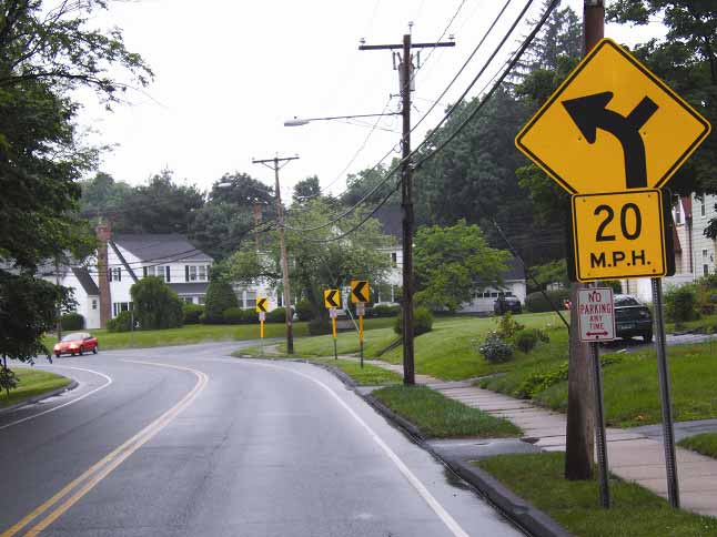
One such strategy with potential for improving horizontal curve safety is enhancing delineation along the curve. According to the National Cooperative Highway Research Program (NCHRP) Report 500 Series, Volume 7, "A Guide for Reducing Collisions on Horizontal Curves," enhancing delineation along the curve is currently a tried but not proven strategy that can be implemented on most curves as well as problem curves.⁽²⁾ Enhanced curve delineation can serve multiple purposes. It allows for better visibility while approaching curves by increasing visual cues to drivers when they are approaching a curve. In addition, it provides positive guidance while navigating through curves. Improved delineation can be helpful in encouraging drivers to decrease their speed into and through curves, reducing the frequency of run-off-road or head-on crashes. Last, improving delineation can especially be helpful under low light or dark conditions.

Options for enhanced delineation include using better pavement markings, such as markings with higher durability, all-weather quality, or higher retroreflectivity. Other options include post-mounted delineators, chevrons, raised pavement markers, and wider edge lines.⁽²⁾ An example of enhanced curve delineation is shown in figure 1.

Figure 1. Photo. Example of a curve treated with enhanced delineations in Connecticut.

Enhanced delineation is a potential treatment for curves that have some form of delineation or other safety treatment but continue to experience higher crash rates.⁽¹⁾ The installation or upgrade of pavement markings should follow the guidelines in the Manual on Uniform Traffic Control Devices (MUTCD).⁽⁴⁾

BACKGROUND ON STUDY

In 1997, the AASHTO Standing Committee for Highway Traffic Safety, with the assistance of the FHWA, the National Highway Traffic Safety Administration (NHTSA), and the Transportation Research Board (TRB) Committee on Transportation Safety Management, met with safety experts in the field of driver, vehicle, and highway issues from various organizations to develop a strategic plan for highway safety. These participants developed 22 key areas that affect highway safety. One of these areas focuses on crashes on horizontal curves.

The NCHRP published a series of guides to advance the implementation of countermeasures targeted to reduce crashes and injuries. Each guide addresses 1 of the 22 emphasis areas and includes an introduction to the problem, a list of objectives for improving safety in that emphasis area, and strategies for each objective. Each strategy is designated as proven, tried, or experimental. Many of the strategies discussed in these guides have not been rigorously evaluated-about 80 percent of the strategies are considered tried or experimental.

The FHWA organized a pooled fund study of 26 States to evaluate low-cost safety strategies as part of this strategic highway safety effort. The purpose of the pooled fund study is to evaluate the safety effectiveness of several tried and experimental low-cost safety strategies through scientifically rigorous crash-based studies. Improving delineation on horizontal curves was selected as a strategy to be evaluated as part of this effort.

LITERATURE REVIEW

According to the NCHRP Report 500 Series, Volume 7, "A Guide for Reducing Collisions on Horizontal Curves," although general conclusions can be drawn, no quantitative estimates of the effects of the safety effectiveness of enhancing delineation along curves can be made.⁽²⁾ Fitzpatrick et al. indicated that post-mounted delineators lower the crash rate at night for relatively sharp curves; however, the study did not quantify the effect of the same treatment on other curves.⁽⁵⁾ Zador et al. conducted a study examining the effect of chevrons, post-mounted delineators, and raised pavement markers on the speed and placement of vehicles on two-lane rural highways.⁽⁶⁾ The study showed that a primary benefit of these treatments is to help drivers notice when they are nearing a curve. Studies conducted by Agent and Creasely found that pavement markings had a greater effect on drivers than post-mounted delineators and that chevrons had a larger influence on speed and encroachments than post-mounted delineators.⁽⁷⁾ Jennings and Demetsky evaluated three post-mounted delineator systems based on changes in speed and lateral placement of vehicles in the travel lanes.⁽⁸⁾ They concluded that drivers react most favorably to chevron signs on sharp curves greater than or equal to 7 degrees and to standard delineators on curves less than 7 degrees.

A 2004 study conducted by Gates et al. analyzed the impacts of various sign conspicuity enhancements on traffic operations and driving behavior.⁽⁹⁾ The evaluation was comprised of 14 sites in Texas. Six different fluorescent applications were chosen for this evaluation, which included yellow chevrons, yellow chevron posts, yellow curve signs, yellow ramp advisory speed signs, yellow "Stop Ahead" signs, and red stop signs. Two additional applications including flashing red light-emitting diode stop signs and standard red borders on speed limit signs were studied. Fluorescent yellow chevron signs were found to cause a reduction in edge line encroachments as well as curve speed. This investigation yielded valuable results, but the study was limited in that it did not examine the possible beneficial impacts on crashes but focused on safety surrogates.

In 2006, FHWA released Low-Cost Treatments for Horizontal Curve Safety, a resource providing practical information on low-cost treatments that can address identified or potential safety problems at horizontal curves.⁽¹⁰⁾ Although it is a useful resource for horizontal curve improvements, it does not contain conclusive quantitative estimates of the safety effectiveness of enhancing delineation treatments along curves.

A 2006 study by Opiela et al. evaluated the effectiveness of roadway delineation at a variety of curves.⁽¹¹⁾ Sixteen research participants drove an instrumented FHWA test vehicle for a consecutive 8-night period. Each night, various curves were treated with different combinations of pavement markings, pavement markers, and horizontal signage. The research participants rated the effectiveness of the roadway delineation on each curve. The study recorded positive results for increasing retroreflectivity of pavement markings and horizontal signage. Wider edge lines along with the installation of horizontal curve warning signage also achieved desirable results. While this investigation yielded valuable results, it did not investigate the impacts on crashes.

A 2007 study by Charlton tested two groups of curve treatments using a driving simulator.⁽¹²⁾ One group consisted of treatments to warn drivers before driving through the curve, and the other group focused on treatments to reduce driver speed while driving through the curve. The results indicated that advance warning signs by themselves were not as effective at reducing driver speeds as when they were used in conjunction with chevron sight boards and/or repeater arrows. However, this study focused on attention, perceptual, and lane placement factors. It did not include effects on crashes.

A 2009 study by Montello evaluated the safety effectiveness of treatments aimed at improving horizontal curve delineation on 15 curves on the A16 Naples-Canosa motorway in Italy. Montello indicated that all the curves are characterized by low radius and high deflection angle, limited sight distance, and limited super elevation.⁽¹³⁾ Treatments involved installation of chevron signs, curve warning signs, and sequential flashing beacons along the road. An EB observational before-after study was performed. There was a statistically significant reduction in total, nighttime, daytime, rainy, non-rainy, run-off-road, and property damage only crashes. Total crashes decreased by 39.4 percent. The treatment was more effective in curves with radii less than or equal to 984 ft and with deflection angles greater than 54 degrees. The results of this study clearly indicate that improving curve delineation can provide significant benefits, although it is not clear if these results can be translated to conditions in the United States. In addition, the focus of Montello's study was on access-controlled four-lane divided roads, unlike the two-lane rural roads that are investigated in this low-cost pooled fund effort.⁽¹³⁾

The results of this literature review support the NCHRP Report 500 Series statement that this strategy cannot be considered proven because there were no truly valid estimates of the effectiveness based on sound before-after crash-based studies in the United States. More research is needed to substantiate these and other evaluations for highway agencies implementing the strategy to be confident that they are applying their resources effectively.

OBJECTIVES

This study examined the safety impacts of improved delineation through signing improvements on horizontal curves using the EB method. Target crash types included the following:

• Total non-intersection crashes.
• Non-intersection lane departure crashes.
• Injury and fatal non-intersection crashes (K, A, B, and C injuries on KABCO scale, which is used to represent injury severity in crash reporting).
• Non-intersection crashes during dark conditions.
• Non-intersection lane departure crashes during dark conditions.

A second objective was to determine whether the effects varied by the following:

• Traffic volume.
• Curve radius.
• Type of treatment, e.g., installation of new signs versus replacement of old signs.

The final objective was to estimate the overall effectiveness of the strategy. Meeting these objectives placed some special requirements on the data collection and analysis tasks including the following:

• The need to select a large enough sample size to detect, with statistical significance, what may be small changes in safety for some crash types.
• The need to identify appropriate reference sites.
• The need to properly account for traffic volume changes.
• The need to pool data from multiple jurisdictions to improve reliability of the results and facilitate broader applicability of the products of the research.

STUDY DESIGN

The study design involved a sample size analysis and prescription of needed data elements. The sample size analysis assessed the sample size required to statistically detect an expected change in safety, and it also determined what changes in safety could be detected with likely available sample sizes.

SAMPLE SIZE OVERVIEW

Minimum and desired sample sizes were calculated assuming a conventional before-after study with a comparison group, as described in Hauer.⁽¹⁴⁾ The sample size estimates were conservative because the EB methodology was incorporated in the before-after analysis rather than applied in a conventional before-after analysis with a comparison group.

Sample sizes were estimated for assumptions of likely safety effects and crash frequencies in the before period. Based on information from the horizontal curves without the treatment in Connecticut, average crash rates were calculated for three crash types, which included the following:

• Non-intersection crashes: 6.96 crashes per mile per year.
• Non-intersection lane departure crashes: 4.86 crashes per mile per year.
• Non-intersection crashes during dark conditions: 2.56 crashes per mile per year.

To facilitate the analysis, it was also assumed that the number of reference sites was equal to the number of strategy sites. The sample size estimates provided would be conservative in that stateof-the-art EB methodology proposed for the evaluations would require fewer sites.

Table 1 provides estimates of the required number of before and after period mile-years for both the 90-percent and 95-percent confidence levels. Mile-years are the number of miles of roadway on which the strategy was applied multiplied by the number of years the strategy was in place. For example, if a strategy is applied on 9 mi of roadway and has been in place for 3 years on all 9 mi, there are 27 mile-years.

The minimum sample indicates the level for which a study seems worthwhile; that is, it is feasible to detect with 90-percent confidence the largest effect that may reasonably be expected based on what is currently known about the strategy. In this case, a 20-percent reduction in crashes was assumed as this upper limit on safety effectiveness. The desirable sample assumes that the reduction could be as low as 10 percent for total crashes, and this is the smallest benefit that one would be interested in detecting with 90-percent confidence. The logic behind this approach is that safety managers may not want to implement a measure that reduces crashes by less than 10 percent, and the sample size required to detect a reduction smaller than 10 percent would likely be prohibitively large. The sample size calculations for this study were based on specific assumptions regarding the number of crashes per mile-year.

The minimum and desirable sample size depends on the target crash type that is selected. The two primary target crash types are total number of non-intersection lane departure crashes and non-intersection crashes during dark conditions. Depending on which crash type is selected, the minimum sample size is either 37 or 71 mile-years, and the desirable sample size is either 183 or 348 mile-years (shown in bold in table 1). As mentioned earlier, the calculations assume an equal number of mile-years for the strategy and reference sites and an equal length of before and after periods. These selections assume that the reduction in crashes in each case could be as low as a 10-percent reduction in all crashes and that this is the smallest benefit that one would be interested in detecting with 90-percent confidence. Estimates may be predicted with greater confidence, or a smaller reduction in crashes may be detectable if it turns out that there are more mile-years of data available in the after period. The same holds true if there is a higher crash rate than expected in the before period.

Table 1. Minimum required before period mile-years for treated sites.

Note: The bold numbers denote the desirable sample size.

METHODOLOGY

The EB methodology for observational before-after studies was used for the evaluation.⁽¹⁴⁾ This methodology is rigorous in that it addresses the following:

• It properly accounts for regression-to-the-mean.
• It overcomes the difficulties of using crash rates in normalizing for volume differences between the before and after periods.
• It reduces the level of uncertainty in the estimates of safety effect.
• It provides a foundation for developing guidelines for estimating the likely safety consequences of contemplated strategy.
• It properly accounts for differences in crash experience and reporting practices in amalgamating data and results from diverse jurisdictions.

In the EB approach, the change in safety for a given crash type at a site is given by the following:

(1)

Δ Safety = λ - p

Change in safety.
Change in safety equals lambda minus pi.

Where:

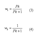
λ = The expected number of crashes that would have occurred in the after period without strategy.
p = The number of reported crashes in the after period.

In estimating λ, the effects of regression-to-the-mean and changes in traffic volume were explicitly accounted for using safety performance functions (SPFs) relating crashes of different types to traffic flow and other relevant factors for each jurisdiction based on untreated sites (reference sites). Annual SPF multipliers were calibrated to account for the temporal effects (e.g., variation in weather, demography, and crash reporting) on safety.

In the EB procedure, the SPF is used to first estimate the number of crashes that would be expected in each year of the before period at locations with traffic volumes and other characteristics similar to the one being analyzed (i.e., reference sites). The sum of these annual SPF estimates (P) is then combined with the count of crashes (x) in the before period at a strategy site to obtain an estimate of the expected number of crashes (m) before strategy. This estimate of m is as follows:

(2)

m = w₁(x) + w₂(P)

m.
m equals the product of w subscript 1 times x
plus the product of w subscript 2 times P.

Where the weights w₁ and w₂ are estimated from the mean and variance of the SPF, estimate as follows:

Where:

k = A constant for a given model, and it is estimated from the SPF calibration process with the use of a maximum likelihood procedure. In that process, a negative binomial distributed error structure is assumed with k being the dispersion parameter of this distribution.

A factor is then applied to m to account for the length of the after period and differences in traffic volumes between the before and after periods. This factor is the sum of the annual SPF predictions for the after period divided by P, the sum of these predictions for the before period. After applying this factor, the result is an estimate of λ. The procedure also produces an estimate of the variance of λ.

The estimate of λ is then summed over all sites in a strategy group of interest (to obtain λ_sum) and compared with the count of crashes during the after period in that group ( π_sum). The variance of λ is also summed over all sites in the strategy group.

The Index of Effectiveness (θ) is estimated as follows:

₍₅₎

The standard deviation of θ is given by the following:

(6)

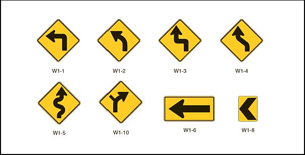
The percent change in crashes is calculated as 100(1-θ). Thus, a value of θ= 0.7 with a standard deviation of 0.12 indicates a 30-percent reduction in crashes with a standard deviation of 12 percent.

DATA COLLECTION

CONNECTICUT

Background

Connecticut provided installation data, including locations and dates for installations of improved signing on horizontal curves. It also provided roadway characteristics data, traffic volumes, and crash data for both the installation and reference sites. This section provides a summary of the data assembled for the analysis.

The Connecticut Department of Transportation (ConnDOT) used fluorescent yellow sheeting to improve signing at horizontal curves between 2002 and 2006. These curves were selected through a regular program called the Suggested List of Surveillance Study Sites (SLOSSS). SLOSSS uses crash data, traffic volumes, and roadway characteristics to identify intersections and road segments with higher than expected crash rates. District engineers were asked to indicate which of the SLOSSS were located on horizontal curves, and these curve locations were then treated with improved signing. After these were implemented, the ConnDOT received positive feedback from enforcement officials who then asked to have these installed at additional curves.

The treatments used in Connecticut consisted of improved signing using fluorescent yellow sheeting. This included installing new signs or replacing existing signs. The signs in question were either warning signs (e.g., curve ahead or suggested speed limit) and/or curve delineation signs (e.g., chevrons or horizontal arrows). Figure 2 shows the types of signs used in the treatment. Signs W1-1, W1-2, W1-3, W1-4, W1-5, and W1-10 were classified as warning signs in this study. Signs W1-6 and W1-8 were classified as curve delineation signs.

Figure 2. Chart. Sign types used in Connecticut horizontal curve treatments from MUTCD.

The unit cost of a fluorescent yellow sign in Connecticut ranged from $30 to $160 depending on the size of the sign. Smaller signs such as chevrons and advisory speed signs were cheaper than larger signs such as curve warning signs.

Installation Data

ConnDOT provided information on 34 curve treatment projects; each project had between 1 and 16 individual horizontal curves, providing a total of 91 treated horizontal curves. Two curves were excluded from the analysis because their curve radii could not be obtained. This resulted in a sample of 89 curves for further analysis. Service memorandums for each project gave details on the treatment description, installation date, treatment cost, and the number of warning and curve delineation signs that were replaced or newly installed.

Reference Sites

In order to account for biases in treatment site selection, the study analysis required the identification of reference sites. Reference sites were curves that were similar to the treatment sites but did not receive the improved signing treatment. Reference sites were identified in this study by first identifying curves that were located within 1.55 mi of the treatment curves. These curves were then filtered down based on certain exclusion criteria. These criteria ensured that the final list of reference sites would be an appropriate match to the group of treatment sites. Curves that were not included in the final group of reference sites contained the following characteristics:

• Right-turn lane.
• Left-turn lane.
• Center-turn lane (two-way left-turn lane).
• Median.
• More than two travel lanes.
• Radius under 32.8 ft or over 3,280 ft.
• Heading change of less than 2 degrees.

The final group of reference sites included 334 horizontal curves. The total length of the curves in the reference group was 23.6 mi.

Roadway Data

Roadway characteristics data were collected by an instrumented vehicle that drove the entirety of the Connecticut State highway system. One of the most useful pieces of data from this vehicle was the photolog. The vehicle took photos every 32.8 ft along the route in each direction. The photolog was used to visually obtain data on the following items:

• Number of lanes (through, right-turn, left-turn, and center-turn lanes).
• Number of driveways and public street access points.
• Median presence and type.
• Shoulder type and width.
• RHR (1-7 scale).
• Speed limit (regulation).
• Suggested curve speed (if any).
• Cable barrier/guardrail.

Another key piece of data collected by the vehicle was horizontal alignment data. Geographic positioning system (GPS) coordinates taken at regular intervals allowed the vehicle to track the horizontal alignment of the road. An algorithm was later run on the GPS data to divide the road into segments and determine where tangents, arcs, and spirals began and ended. It also calculated the curve radius and degree of heading change from one tangent to the next.

The vehicle also took readings for super-elevation and grade at regular intervals. For unknown reasons, super-elevation data were only available for 40 out of 91 treatment sites and 194 out of 334 reference sites. Grade data were available for all sites.

Traffic Data

Traffic volume counts are performed once every 3 years for each Connecticut road. These average daily traffic (ADT) values are recorded on ADT maps. Maps from 1997 to 2005 were made available to the research team in addition to an electronic file of 2006 ADT data. Team members located each treatment site on the map and took the reading of the nearest ADT count point. In the case of a site lying between two ADT count points, the average value was taken. Since reference sites were chosen in close proximity to treatment sites, any particular reference site was assumed to have the same ADT as its treatment site.

Crash Data

Connecticut crash data from 1995 to 2006 were obtained from the University of Connecticut. Crash data for 2007 were not available at the time of this study.

WASHINGTON

Background

Unlike Connecticut, the treatments in Washington only involved the installation of chevrons (W1-8 signs) on horizontal curves. This included both installation locations where there were previously no chevrons and where the number of chevrons was increased. The Washington State Department of Transportation (WSDOT) provided information on the location of chevrons. Information on traffic volume, roadway characteristics, and crashes were obtained from the Highway Safety Information System (HSIS). The following section of this report provides a summary of the data assembled for the analysis. The cost of each chevron sign was estimated to be $100.

Installation Data

WSDOT provided the research team with information about locations where chevrons were installed in the last 15 years. The milepost information for the chevrons was from a different milepost system than the roadway inventory. WSDOT provided information on converting between the two systems. The project team used these converted mileposts to tie the location of the chevrons with the beginning and ending mileposts of horizontal curves in the HSIS system. The project team identified 139 curves on rural two-lane roads where chevrons were installed sometime between 1994 and 2006.

Reference Sites

HSIS data were used to identify curves on rural two-lane roads that could serve as reference sites. The initial set of reference sites included about 4,000 curves that experienced approximately 8,000 crashes between 1993 and 2007. Several alternative reference groups were examined to obtain the reference group most similar to the treatment group in its characteristics. Further detail about the different reference groups is available in the appendix.

Roadway Data

From HSIS, the following information was compiled for each reference curve over the study period:

• Average annual daily traffic (AADT).
• Curve length.
• Curve radius.
• Shoulder width.
• Lane width.
• Percent grade.
• Terrain.

In situations where a particular characteristic (e.g., shoulder width) varied within a curve, an average value was computed for each curve. There is some evidence to indicate that curves separated by short tangent sections may have more accidents compared to curves that are separated by long tangent sections. Therefore, the distance between consecutive curves was desired. The initial effort to obtain the distance between curves found a large number of long tangent sections (tangent sections exceeding 5 mi). Further review indicated that this counterintuitive result was because of gaps in the data due to coinciding routes. Coinciding routes are two routes that share the roadway section, but the roadway inventory and crash information is available only for one of the routes. Identifying the coinciding routes required the project team and HSIS staff to review individual roadway sections from the raw data provided by WSDOT.

Traffic Data

AADT data were obtained from HSIS for the treatment and reference sites. AADT data were not available from 1999 to 2001. To fill in the missing data, an algorithm developed by Lord was utilized.⁽¹⁹⁾ Upon a cursory review of the AADT, there were several curves where AADT changed dramatically from year to year (for example, one site had an AADT of 138 in 2005 and 7,325 in 2006). The project team only included curves where the difference between the AADT of 2 consecutive years was less than 20 percent to exclude any sites with unreliable AADT.

Crash Data

Crash data were requested from HSIS for the study period starting in 1993 and ending in 2007. Crash data for 1997 and 1998 were not provided to HSIS by WSDOT; therefore, it was not available for analysis in this effort.

SUMMARY OF DATA

In both States, data were compiled for the following crash types:

• Total non-intersection crashes: A non-intersection crash was defined based on the information by the police officer on the location of the crash.
• Non-intersection injury and fatal crashes: This included all non-intersection crashes where there was at least one non-fatal injury or one fatal injury.
• Non-intersection lane departure crashes: Lane departure crashes included sideswipe, overturn, head-on, jackknife, and run-off-road.
• Non-intersection crashes during dark conditions: This category included crashes for which the light condition was coded as "dark-not lighted" or "dark-lighted."
• Non-intersection lane departure crashes during dark conditions: This category included crashes that were lane departure but with the light condition coded as "dark-not lighted" or "dark lighted."

Table 2 shows the summary of the data collected in Connecticut. Table 3 shows the summary of the data collected in Washington.

Table 2. Data summary for Connecticut (89 curves, 7.08 mi).

Table 3. Data summary for Washington (139 curves, 14.06 mi).

Connecticut has more crashes per mile per year than Washington. The average AADT is also about 30 percent higher in Connecticut. Looking at the injury and the total crash numbers in both States, a higher percentage of crashes in Washington are injury as compared to crash types in Connecticut.

The total available sample of 117.3 mile-years in the before period and 116.6 mile-years in the after period are higher than the minimum sample of 37 mile-years for non-intersection lane departure crashes and the minimum sample size of 71 mile-years for non-intersection crashes during dark conditions but less than the desirable sample sizes for both these crash types. However, it is important to note that actual crash rates in the before period are higher in Connecticut (for both non-intersection lane departure crashes and non-intersection crashes during dark conditions) and lower in Washington (for the same crash types) than the rates assumed in the study design. The average crash rates from the two States for the two crash types are slightly higher than the rates assumed in the study design. Hence, it is safe to assume that the sample size is adequate for both these two crash types and to proceed with the analysis.

DEVELOPMENT OF SAFETY PERFORMANCE FUNCTIONS

This section presents the methodology used to estimate the SPFs. The SPFs are used in the EB methodology to estimate the safety effectiveness of this strategy.⁽¹⁴⁾ Generalized linear modeling was used to estimate model coefficients using the software package SAS^® assuming a negative binomial error distribution, which is consistent with the state of research in developing these models.⁽¹⁵⁾ The over-dispersion parameter, k, is also estimated by SAS^® in the model calibration process. The over-dispersion parameter relates the mean and variance of the SPF estimate and is such that the smaller its value, the better a model it is for a given set of data. Thus, it is a useful criterion in comparing candidate models.

The form of the SPFs is as follows:

(7)

Where:

X = The independent variables.
ß = Parameters to be estimated.

Table 4 shows the independent variables that were available for the models in the two States.

Table 4. Variables considered for inclusion in the SPFs.

The developed SPFs are presented in the appendix. While estimating the SPFs, if a variable did not significantly improve the model, it was eliminated. To account for the effect of changes in factors such as weather, crash reporting practices, and demography over time, annual factors were estimated for each year. The annual factor for a particular year is defined as the ratio of observed to predicted crashes for that year. Annual factors for all five models were estimated based on the SPFs developed for total crashes.

RESULTS

Two sets of results are provided below: aggregate and disaggregate. The aggregate analysis provides evidence for the general effectiveness of the strategy, while the disaggregate analysis provides insight on the situations where the strategy may be most effective.

AGGREGATE ANALYSIS

The aggregate results are present in table 5 through table 7 for Connecticut, Washington, and the two States combined, respectively. The tables provide the EB estimate of the crashes expected in the after period if the treatment had not been installed, the actual number of crashes in the after period, and two measures of change. The first measure of safety effect is the estimated percent reduction due to the strategy along with the standard error (SE) of this estimate-a negative value would indicate an increase in crashes. If the magnitude of the percent change is at least 1.96 times higher than the SE, then the change is statistically significant at the 95-percent confidence level. Those safety effects that are significant at the 95-percent confidence level are denoted by bold text. The second measure of safety effect is the change in the number of crashes per mile-year, which is calculated as the difference between the EB estimate of crashes expected in the after period and the count of observed crashes in the after period divided by the number of mile-years in the after period.

In Connecticut, there was a statistically significant reduction at the 95-percent confidence level in all the crash types that were evaluated. Total non-intersection and non-intersection lane departure crashes were reduced by approximately 18 percent. Injury and fatal non-intersection crashes were reduced by about 25 percent. The percentage reduction was larger (35 percent) for the crashes that occurred during dark conditions.

In Washington, there was a statistically significant reduction in crashes during dark conditions and lane departure crashes during dark conditions. The reduction for these two crash types exceeded 20 percent. The combined results presented in table 7 for the two States indicate a statistically significant reduction in injury and fatal crashes, crashes during dark conditions, and lane departure crashes during dark conditions.

Table 5. Results from Connecticut sites.

Note: Bold denotes results that are statistically significant at the 95-percent confidence level.

Table 6. Results from Washington sites.

Note: Bold denotes results that are statistically significant at the 95-percent confidence level.

Table 7. Combined results from Connecticut and Washington.

Note: Bold denotes results that are statistically significant at the 95-percent confidence level.

DISAGGREGATE ANALYSIS

The disaggregate results are presented in table 8 through table 11. The disaggregate analysis focused on the following factors:

• Average AADT at a site before treatment.
• The radius of the curve where the treatment was implemented.
• The RHR at the treatment site.
• The number of signs in advance of the curve that were added or replaced.
• The number of within-curve signs that were added or replaced.

AADT and curve radius were available from both Washington and Connecticut. The RHR and the number of signs were available only in Connecticut.

Curve radius was examined with combined data from Washington and Connecticut. There were no clear trends regarding the effectiveness of the treatment with respect to the radius of the curve. Curve radius was also examined in the two States separately. In Washington, there were no clear trends regarding the effectiveness of the treatment with respect to the radius of the curve. However, in Connecticut, the treatments seem to have been more effective in sharper curves (radius less than 0.093 mi) compared to flatter curves (radius equal to or exceeding 0.093 mi; see table 9).

When the RHR was examined using data from Connecticut, the results indicated that the treatments were more effective at sites with more hazardous roadsides (RHR of 5 or 6) compared to less hazardous roadsides (RHR between 2 and 4) for crashes during dark conditions and lane departure crashes during dark conditions (see table 10).

When the effect of the number of signs in advance of the curve (added or replaced) was examined using data from Connecticut, there was no clear trend in terms of safety. However, when the number of within-curve signs (added or replaced) was examined, sites with more signs added or replaced (more than seven per curve) seemed to have experienced a larger reduction in crashes compared to sites where fewer signs were added or replaced (less than or equal to seven per curve).

Finally, there were indications that the treatment was more effective for sites with higher AADT compared to sites with lower AADT.

Table 8. Results of the disaggregate analysis using curve radius in Connecticut.

1 m = 3.28 ft
Note: Bold denotes results that are statistically significant at the 95-percent confidence level.

Table 9. Results of the disaggregate analysis using RHR in Connecticut.

Note: Bold denotes results that are statistically significant at the 95-percent confidence level.

Table 10. Results of the disaggregate analysis using the number of within-curve signs added or replaced in Connecticut.

Note: Bold denotes results that are statistically significant at the 95-percent confidence level.

ECONOMIC ANALYSIS

Table 11 summarizes the results of the economic analysis. A combined economic analysis is provided, but separate analyses are also provided for each State, as each State has its own variation of the treatment. The annualized cost of the treatment is first computed based on information provided by Connecticut and Washington. Connecticut provided costs based on the type of treatment, ranging from $30 to $160 for a fluorescent yellow sign with a service life of 5 years. The unit cost varied depending on the size of the sign; smaller signs such as chevrons and advisory speed signs were less expensive than larger signs such as curve warning signs. Washington provided an estimate of $100 for chevrons. The lower and upper limits from Connecticut were used to provide a range of cost estimates, but the cost may vary for other States depending on the size of the sign and installation and maintenance practices.

The formula to calculate the annual cost is as follows:

(8)

Where:

C = Installation cost.
R = Discount rate (as a decimal).
N = Expected service life (years).

Based on information from the Office of Management and Budget, a discount rate of 2.4 percent was used to determine the annual cost of the strategy.⁽¹⁷⁾ Assuming installation costs of $30 per sign, this equates to an annualized cost of $6.44 per sign. Although the number of warning signs per curve may vary, it was assumed that 10 chevron signs were installed per curve, resulting in an annual treatment cost per curve of $64. Assuming installation costs of $160 per sign, the annualized cost is $34.34 per sign and an annual treatment cost of $343 per curve. Consequently, the required annual crash savings ranges from $128 to $686 per curve to achieve a 2:1 benefit-cost ratio.

The most recent FHWA mean comprehensive crash costs were used to estimate the cost for a lane departure crash based on 2001 dollar values.⁽¹⁸⁾ The FHWA crash cost document does not directly report the cost for a lane departure crash, so the cost was estimated based on the cost of lane departure-related crashes and the percentage of these crashes. Lane departure- related crashes include head-on, sideswipe, single-vehicle rollover, and single-vehicle fixed object crashes. Based on Washington crash data, these crashes represent 2.6, 1.6, 25.9, and 69.9 percent, respectively. The mean comprehensive crash costs for these crash types are $60,451, $16,019, $147,629, and $67,353, respectively, assuming a speed limit less than 45 mi/h. A weighted average was computed by combining the crash costs with the percentage of each crash type, resulting in a cost of $87,143 per lane departure crash.

Crash savings were computed based on the results for non-intersection lane departure crashes during dark conditions. The total crash reduction was calculated for each State by subtracting the actual crashes in the after period from the expected crashes in the after period had the treatment not been implemented. Crashes per site-year were calculated by dividing the total crash reduction by the number of site-years for each State. Site-years, which are computed similarly to mile-years, are the number of sites multiplied by the number of years of installation. The benefit (i.e., crash savings) is the product of the total crash reduction per site-year and the cost of a lane departure crash (i.e., $87,143). The benefit-cost ratio indicates a range for which the lower and upper limits represent assumed installation costs of $160 and $30 per sign, respectively.

Table 11. Summary of economic analysis results.

Even with the conservative assumptions made, a very modest reduction in crashes is required to justify this strategy economically. The benefit-cost ratios reported in table 11 far exceed a 2:1 benefit-cost ratio. While the cost of the strategy may vary by State, it is likely that the annualized costs will not exceed the annual crash savings. Therefore, this strategy is justified economically.

SUMMARY AND CONCLUSION

The objective of this study was to evaluate the safety effectiveness of improved delineation on horizontal curves through signing improvements. The results of the aggregate analysis using data from Connecticut and Washington indicated a statistically significant reduction in injury and fatal crashes (18-percent reduction), crashes during dark conditions (27.5-percent reduction), and lane departure crashes during dark conditions (25.4-percent reduction). Table 12 presents the recommended crash reduction factors and SEs. Based on the limited data from Connecticut, the reductions in crashes were more prominent on sharper curves (curve radius less than 492 ft) and in locations with more hazardous roadsides (RHR of 5 or higher) compared to locations with less hazardous roadsides (RHR of 4 or lower). In addition, curves where more within-curve signs were either added or replaced (with a more retroreflective material) experienced larger reductions in crashes. In both States, the reductions appeared to be more prominent at locations with higher traffic volumes. An economic analysis revealed that improving curve delineation with signing improvements is a very cost-effective treatment with the benefit-cost ratio exceeding 8:1.

Table 12. Crash reduction factors (CRFs) for improving curve delineation through
signing improvements.

APPENDIX: SAFETY PERFORMANCE FUNCTIONS

This appendix provides the SPFs estimated in Connecticut and Washington. As mentioned previously, the form of the SPFs is as follows:

(9)

Where:

X = The independent variables.

ß = Parameters to be estimated.

The tables in the appendix show the independent variable, ß , the SE for ß , the over-dispersion parameter, k, some summary statistics, and goodness-of-fit information. The yearly factors derived from the observed crash counts and predicted crash counts are also shown. For Washington, there is also a discussion of the alternative reference groups that were considered.

Table 13. SPFs from Connecticut.

1 m = 3.28ft
1 km = 0.621 mi
Note: The estimate value is shown first with the SE following in parentheses.
Blank cells indicate that the variable was not included in the particular model (i.e., for a specific crash type).

Table 14. Yearly factors for Connecticut SPFs.

SAFETY PERFORMANCE FUNCTIONS FOR WASHINGTON SITES

In Washington, a special procedure was required to ensure that the reference group was representative of and comparable to the treatment group. Initially, a large reference group of curves on rural two-lane roads from all over the State was used to estimate the SPFs. When the results of these SPFs were used to predict the number of crashes in the treatment group before the installation of the treatment, the predicted crashes were unexpectedly much lower compared to the actual number of crashes before treatment (144 crashes were predicted compared to 314 crashes that actually occurred during that period). This difference is much larger than might be expected due to regression to the mean, especially considering that the before period averaged about 5 years. Next, the research team sought to ensure that the reference group was indeed similar to the treatment group in terms of characteristics that were available (e.g., AADT, curve radius, and terrain) and characteristics that were not available (e.g., roadside characteristics and climate). To this end, the help of HSIS staff was sought to identify curves on the same route in close proximity to the treatment curves. This investigation lead to two additional potential reference groups: one group with curves within 5 mi of treatment curves and the other within 2 mi of the treatment curves. By selecting curves in close proximity to the treatment group, it was determined that the characteristics such as roadside characteristics and climate would be similar in the treatment and reference groups. SPFs were developed with data from these two additional reference groups; however, the results from these SPFs did not produce better predictions. In fact, 135 crashes were predicted, which was slightly lower than the 144 crashes that were predicted by the larger statewide reference group.

The next step was to explore the possibility of matching the distribution of critical independent variables in the reference and treatment groups. Although these critical variables were included in the SPFs, it was concluded that matching the distributions would provide better predictions, considering that the functional form of these independent variables in the SPFs may not always correspond to their true functional form. AADT and curve radius were considered the most critical variables in the models.

The distribution of AADT was similar in the treatment and reference groups. However, the median and mean curve radii were much lower in the treatment group compared to the reference groups, indicating that the reference groups had a larger percentage of curves with a higher radius (the range of curve radius was the same in all groups). Curve radius was divided into seven categories, which included the following:

• Radius less than or equal to 500 ft.
• Radius is between 501 ft and 1,000 ft.
• Radius between 1,001 ft and 1,500 ft.
• Radius between 1,501 ft and 2,000 ft.
• Radius between 2,001 ft and 2,500 ft.
• Radius between 2,501 ft and 3,000 ft.
• Radius between 3,001 ft and 4,000 ft.

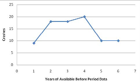
Curves were randomly selected by using a random number generator and removed from the statewide reference group so that the percentage of curves within the seven categories was similar in the treatment and statewide reference group. The revised statewide reference group was used to estimate the SPFs. The predicted number of crashes was marginally higher (153 versus 144 from the original statewide reference group), but it was still substantially lower than the 314 crashes that actually occurred during the same period. WSDOT was contacted regarding this apparent anomaly, but they were not able to provide further insight.

This exercise seemed to indicate that the treatment curves were unique for some unknown factors that were not reflected in the reference group data. To proceed with an analysis that would recognize this uniqueness and be defendable, the SPFs developed using the revised statewide reference group were calibrated to be more representative of the treatment group. The total number of crashes in the treatment group in the first year before treatment through the sixth year before treatment were plotted to identify if there was any evidence of randomly high crashes during any of these periods. Only those sites that had data for 6 consecutive years before the treatment were included in this plot. In Washington, crash data were not available in 1997 and 1998, and hence, only sites where the treatment was implemented in 2006 or 2005 provided 6 consecutive years before the implementation of the treatment. Data from 25 sites (out of 139 sites) were included in the plot in figure 3.

Figure 3. Graph. Crashes for 25 site-years of available before period data.

This plot suggests that crash counts in the 5 years before treatment may have been randomly high, but this apparent selection bias seemed to disappear for curves with 5 or more years before treatment. Based on this observation, it was decided that using curves with 5 or more years of data before treatment for the calibration would minimize the possibility of bias due to regression to the mean. This decision was also supported by anecdotal evidence that there was a tendency to follow the rule of thumb of selecting high crash sites for treatment based on no more than the most recent 5 years of data.

To further examine whether regression to the mean may have influenced the results of the evaluation, the research team conducted a before-after study (with a comparison group) where data for 5 years before the treatment, which were likely subject to regression to the mean bias, were excluded from all the sites. Consequently, sites with less than 6 years of before data were excluded from this examination. In this before-after study with a comparison group, the expected crashes in the after period were computed as follows:

Expected crashes in the after period = (Observed crashes in the before period)* SPF_a / SPF_b (10)

Where:
SPF_a = The number of crashes predicted in the after period in these sites by the SPF estimated with the statewide data.

SPF_b = The number of crashes predicted in the before period in these sites by the same SPF.

Thus, the actual SPF calibration factor is immaterial since it is in both the numerator and denominator of the above equation. Table 15 compares the results of the EB analysis (reported in the main body of the report) with the before-after study with a comparison group based on before periods 5 or more years before treatment.

Table 15. Comparison of EB analysis with the before-after study with comparison
(based on 5 or more years of before treatment data).

Note: The standard errors are presented in parentheses after the percent reduction.

Table 15 shows that the results from the before-after EB study were very close to (and actually on the conservative side) the results of the before-after study with a comparison group where crashes for 5 years before treatment were eliminated. The similarity between the results provides further evidence that the approach adopted in recalibrating the SPFs using well-before treatment data was a reasonable one.

Having rationalized the calibration of the SPFs to the treatment site data 5 or more years before treatment, this calibration was done for the five different crash types. The SPFs, calibration factors, and estimated over-dispersion parameters are shown in table 16 through table 18.

Table 16. SPFs for total crashes from revised statewide reference group in Washington.

Table 16 is based on 17,078 observations and 1,971 crashes in the reference group. The calculated Freeman Tukey R-square value is 0.099. Note that for this SPF, two AADT terms were included to capture the more complex relationship between crash frequency and AADT. The coefficients for one of the AADT terms was negative, indicating that for high values of AADT, crash frequency may start decreasing, which is a counterintuitive result. In the dataset used for the estimation, the maximum AADT was 15,000, and for AADT not exceeding 15,000, the predicted crash frequency continuously increased with AADT. This model should not be used to predict crashes for sections with AADT exceeding 15,000. SPFs using a similar functional form were estimated by Hauer et al. for four-lane undivided road segments.⁽²⁰⁾

Table 17. Yearly factors for Washington total crash SPF.

Table 18. Calibration with well-before treatment data (at least 5 years prior to treatment installation).

ACKNOWLEDGEMENTS

This report was prepared for the FHWA. The current FHWA Contract Task Order Manager for this project was Roya Amjadi. Kimberly Eccles, P.E., was the study Principal Investigator. Dr. Raghavan Srinivasan was the lead analyst for this strategy and was the primary author of the report. Dr. Bhagwant Persaud and Craig Lyon developed the study design and provided general oversight of the analysis. Dr. Jongdae Baek was the lead programmer on this effort and prepared the data sets for analysis. Nancy X. Lefler and Daniel Carter led the data collection for the study and also contributed sections to the draft report. Charles Hamlett also participated in the data collection. Other significant contributions to the study were made by Dr. Hugh McGee, Dr. Forrest Council, Michelle Scism, and Yusuf Mohamedshah.

The project team gratefully acknowledges the participation of the following organizations and individuals for their assistance in this study:

• The ConnDOT, particularly John F. Carey, Al Iallonardo, and Brad Overturf.
• The University of Connecticut, particularly Hongmei Zhou and John Ivan.
• The WSDOT, particularly Rick Mowlds, Dan Davis, Mark Finch, and John Milton.

REFERENCES

1. National Center for Statistics and Analysis of the National Highway Traffic Safety Administration. (2006). Fatality Analysis Reporting System, Washington, DC. Obtained from: http://www-fars.nhtsa.dot.gov/Main/index.aspx. Last accessed June 21, 2008.
2. Torbic, D.J., Harwood, D.W., Gilmore, D.K., Pfefer, R., Neuman, T.R., Slack, K.L., and Hardy, K.K. (2004). "Guidance for Implementation of the AASHTO Strategic Highway Safety Plan: A Guide for Reducing Collisions on Horizontal Curves," NCHRP Report 500 Series, Vol. 7, Transportation Research Board, Washington, DC.
3. Glennon, J.C., Neuman, T.R., and Leisch, J.E. (1983). Safety and Operational Considerations for Design of Rural Highway Curves, FHWA/RD-86/035, Federal Highway Administration, Washington, DC.
4. Federal Highway Administration. (2003). The Manual on Uniform Traffic Control Devices (MUTCD), Washington, DC. Obtained from: http://mutcd.fhwa.dot.gov/pdfs/2003r1r2/ pdf_index.htm. Last accessed June 18, 2008.
5. Fitzpatrick, K., Balke, K., Harwood, D.W., and Anderson, I.B. (2000). "Accident Mitigation Guide for Congested Rural Two-Lane Highways," NCHRP Report 500 Series, Vol. 44, Transportation Research Board, Washington, DC.
6. Zador, P.H., Stein, S., Wright, P., and Hall, J. (1987). "Effects of Chevrons, Post-Mounted Delineators, and Raised Pavement Markers on Driver Behavior at Roadway Curves," Transportation Research Record 1114, Transportation Research Board, Washington, DC.
7. Agent, K.R. and Creasey, T. (1986). Delineation of Horizontal Curves, Interim Report UKTRP-86-4, University of Kentucky, Lexington, KY.
8. Jennings, B.E. and Demetsky, M J. (1985). "Evaluation of Curve Delineation Sign," Transportation Research Record 1010, Transportation Research Board, Washington, DC.
9. Gates, T.J., Carlson, P.J., and Hawkins Jr., G.H. (2004). "Field Evaluations of Warnings and Regulatory Signs with Enhanced Conspicuity Properties," Transportation Research Record 1862, Transportation Research Board, Washington, DC.
10. McGee, H.W. and Hanscom, F.R. (2006). Low-Cost Treatments for Horizontal Curve Safety, FHWA-SA-07-002, Federal Highway Administration, Washington, DC.
11. Opiela, K.S., Donnell, E.T., Katz, B.J., Molino, J., and Moyer, M. (2006). Field Ratings of Nighttime Delineation Enhancements For Curves, Transportation Research Board Annual Meeting 2006 Paper No. 06-2698, Transportation Research Board, Washington, DC.
12. Charlton, S.G. (2007). "The Role of Attention in Horizontal Curves: A Comparison of Advance Warning, Delineation, and Road Marking Treatments," Accident Analysis & Prevention, 39(5), 873-885.
13. Montello, A. (2009). "Safety Evaluation of Curve Delineation Improvements: an Empirical Bayes Observational Before-After Study," Presented at the 2009 Annual Meeting of the Transportation Research Board, Washington, DC.
14. Hauer, E. (1997). Observational Before-After Studies in Road Safety: Estimating the Effect of Highway and Traffic Engineering Measures on Road Safety, Pergamon Press, Elsevier Science Ltd, Oxford, U.K.
15. SAS^®, SAS Institute Inc., Cary, NC.
    1. Office of Management and Budget. (2008). Discount Rates for Cost-Effectiveness,
    2. Lease Purchase, and Related Analyses: No. A-94 (01/08/2008). Obtained from: https://www.whitehouse.gov/omb/circulars/a094/dischist.pdf. Last accessed March 7, 2009.
16. Zegeer, C.V., Hummer, J., Reinfurt, D., Herf, L., and Hunter, W. (1986). Safety Effects of Cross-Section Design for Two-Lane Roads, FHWA-RD-87-008, Federal Highway Administration, Washington, DC.
17. Council, F., Zaloshnja, E., Miller, T., and Persaud, B. (2005). Crash Cost Estimates by Maximum Police-Reported Injury Severity Within Selected Crash Geometries, FHWA-HRT05-051, Federal Highway Administration, McLean, VA.
18. Lord, D. (2000). "Procedure to Estimate Missing Year-to-Year Traffic Counts at Intersections," 3rd Transportation Specialty Conference of the Canadian Society of Civil Engineering, London, ON.
19. Hauer, E., Council, F.M., and Mohammedshah, Y. (2004). "Safety Models for Urban Four-Lane Undivided Road Segments," Transportation Research Record 1897, 96-105, Transportation Research Board, Washington, DC.