• Federal Highway Administration >
• Publications >
• Research Publications >
• 10038 >
• 005.Cfm >
• Balancing Safety and Capacity in an Adaptive Signal Control System — Phase 1

Balancing Safety and Capacity in an Adaptive Signal Control System — Phase 1

5.0 FINDINGS FROM THE SIMULATION ANALYSIS

As previously noted, Synchro™, VISSIM^®, and SSAM were used to evaluate the effects of different controller parameters on intersection safety. Specifically, the following seven parameters were studied:

• Cycle length.

• Split/phase maximum.

• Offset.

• Detector gap extension timing.

• Left-turn phase treatment (permissive, protected, or combination).

• Left-turn phase sequence (combination of lead and lag).

• Change and clearance intervals (Y+AR).

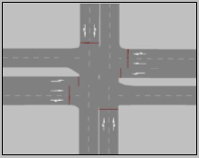
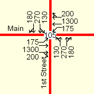
For each parameter, a scenario was defined that was intended to allow the safety aspects (either positive or negative) of that parameter to be observable. The figures of merit used as surrogates for crashes were the estimates of conflicts calculated by SSAM, which produces estimates of conflicts in three categories: crossing, rear end, and lane changing. In general, crossing conflicts reflect the potential for right-angle collisions, rear-end conflicts are correlated with rear-end collisions, and lane-change conflicts are related with sideswipe collisions. A statistically significant change in the average number of conflicts of each type was used as the primary indicator that a given signal timing parameter has an effect on safety.

In order to be able to compare the impact of each signal timing parameter, it was necessary to define a base condition. This baseline was intended to reflect a typical urban arterial intersection operating with peak-hour, but not congested, demand conditions. This process was performed first for an individual intersection and then for a three-intersection arterial.

The remainder of this section defines the base scenario and then compares the results of each of the scenarios with the base condition to determine the impact of each signal timing parameter on the total number of intersection conflicts.

5.1 INTERSECTION BASE CONDITION ANALYSIS

The base condition, as shown in figure 14, reflects the average conditions at a typical urban arterial intersection on a four-lane roadway with left-turn pockets. The base demand condition reflects a relatively high demand typical of a peak hour with a V/C ratio of 0.85. The signal timing optimization program Synchro™ was used to determine optimum signal timing parameters. This combination of intersection geometry and demand is intended to reflect a normal peak-period situation.

Figure 14. Illustration. Typical intersection layout.

The following is a summary of the base condition:

• Demand volumes as shown in figure 15.

• Two through lanes on side streets with shared right- and left-turn lanes.

• Two through lanes on main streets with a shared right-turn lane and a separate left-turn lane.

• Protected lead-lead left-turn phasing.

• Speed limits of 45 mi/h on main street and 30 mi/h on side street.

• V/C ratio of 0.85 for main and side street.

• Link length of 1,000 ft on each of the intersection approaches.

• Detection set per MDSHA standards.⁽¹⁶⁾

• Y+AR set per ITE method.⁽¹⁵⁾

• Signal timing optimized using Synchro™ (resulting in a 65-s cycle length).

• Each simulation conducted for 75 min, including a 15-min warm-up period.

• Six runs performed in VISSIM^®, and trajectory files imported to SSAM.

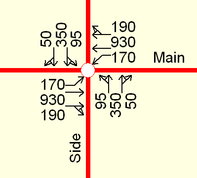
Figure 15. Illustration. Intersection traffic volumes.

Postprocessing the trajectory data from the VISSIM^® runs using SSAM resulted in an average total of 132 conflicts—111 rear-end conflicts, 14 crossing conflicts, and 7 lane-change conflicts (see table 18). There were modest differences in the number of conflicts from one simulation to the next. The fewest number of conflicts was 142, and the maximum number was 185. The coefficient of variation, a measure of the dispersion of the conflict data, was found to be 10.5 percent—a reasonable amount for a stochastic simulation.

Table 18. Summary of conflict data for the intersection baseline analysis.

A further test of 20 iterations was conducted to determine if more iterations would result in larger or smaller standard deviations of the conflict totals. In this test, the average total number of conflicts was 130 and consisted of 113 rear-end, 13 crossing, and 4 lane-change conflicts. The difference between these results and the results of the test using a sample size of six simulations was not statistically significant. Therefore, because of the budget and time constraints of this project, it was determined that a sample size of six 1-h simulations would be adequate to draw statistically significant inferences about the relationships between signal timing and safety. The 1-h simulation for each run was important in order to account for all variations and peak characteristics of traffic and driver behavior within the simulation period. This long simulation period also takes considerable time to run in VISSIM^® and subsequently in SSAM. Therefore, considering that a total of over 400 different runs were conducted in this research, it was important that a proper sample size be selected in order to meet the budget and schedule of the project.

5.1.1 Effects of Changes in Traffic Demand

In the first scenario, the effects of different demand conditions were explored. The demand conditions are expressed in terms of V/C ratios. Three conditions had lower volumes than the base condition (V/C = 0.3, 0.5, and 0.7), and one condition had higher volumes than the base condition (V/C = 1.0). In each case, the signal phasing and cycle length remained the same as the base condition. The cycle length was 65 s, and the split was optimized for each V/C condition. The results, as shown in table 19, indicate that the conflicts were approximately proportional to the volume for this scenario. This is reasonable since one would expect more conflicts as more vehicles are accommodated in the same amount of green time.

Table 19. Average conflicts under different demand conditions.

However, it is interesting to note that the number of conflicts increased more rapidly as the V/C ratio approached 1.0. This is illustrated in table 20 by the increasing ratio of conflicts to V/C as the demand condition increases. This shows that the ratio of demand to capacity is another factor that influences the number of conflicts and, therefore, the potential safety of an intersection.

Table 20. Ratio of conflicts to V/C.

5.1.2 Effects of Changes in Split

In this scenario, the demand was held constant and the signal timings were changed to determine the effect of different splits on conflicts. The splits were adjusted in 10 percent steps from the optimum used in the base condition. The splits were adjusted up and down in proportion to the original split. For example, if the base condition (cycle length = 65 s) had a total green time of 50 s, then the +10 percent simulation would increase the green time by 5 s, resulting in a cycle length of 70 s. The additional 5 s were distributed proportionally among the phases. The results of these simulations are shown in table 21.

Table 21. Conflicts under different split conditions.

This simulation reaffirmed the observation that conflicts increase as the demand-to-capacity ratio increases. The split condition with the least green time (-30 percent) was the condition that experienced the greatest number of conflicts. There is almost an inverse linear relationship between the splits and conflicts. As the split increases, the total number of conflicts decreases. This is not unreasonable since fewer conflicts are expected when the cycle length increases if for no other reason than there are fewer change periods (yellow plus red) per hour with longer cycles. For example, a 50-s cycle will experience 72 change periods per hour while an 80-s cycle will experience 45 change periods per hour. The ratio of maximum to minimum conflicts, 1.8 (175/98), compares well to the ratio of changes, 1.6 (72/45), suggesting that the number of change periods per hour (cycle length) may account for many of the conflicts regardless of other timing parameters. This is illustrated in table 22 with the ratio of conflicts to changes per hour.

Table 22. Ratio of conflicts to changes per hour (various split conditions).

The ratio range is 2.2–2.5 with an average of 2.3 for the seven simulations. This ratio is remarkably stable, indicating that the number of changes per hour accounts for many of the conflicts throughout the range of splits.

The effect of splits on safety was tested by holding the cycle length constant and changing the splits on the main street by borrowing up to 42 percent of the side street split (adding up to approximately 9 s to the main street), borrowing the additional time from the side street beyond its minimum time. The results of this effort are shown in table 23. The same process was followed to generate the conflicts on the side street, the results of which are shown in table 24.

Table 23. Conflicts with main street split adjustments.

Table 24. Conflicts with side street split adjustments.

As shown in table 23, reducing the time available to the main street increased the number of conflicts by approximately 25 percent (80 to 101). The inverse was also true—increasing the time available to the main street reduced the conflicts (80 to 77). However, the reduction was quite small, approximately 4 percent. This suggests that once the optimum green time has been allocated to a phase, there is little to gain by increasing the green time.

Table 24 shows the effect of split changes to the cross street. With this example, the opposite phenomenon was observed—conflicts increased when green time was increased. This may have been the result of the stochastic process employed with the simulation. One possible reason is that most of the conflicts involved vehicles on the main street, and changing the timing on the cross street would have little or no impact on rear-end and lane-change conflicts involving vehicles on the main street.

5.1.3 Effects of Changes in Cycle Length

The initial investigation of splits suggested that the cycle length has a significant impact on the number of conflicts and, thus, on intersection safety. This scenario was intended to directly address the effects of cycle length. In this scenario, five different demand conditions were evaluated. The demand conditions are expressed as the intersection V/C ratio ranging from a low of 0.3 to a maximum of 1.0. All factors remained identical to the base condition except the adjustments to the demand volumes to achieve the various V/C ratios. For each demand condition, the cycle length and splits were optimized. The results of these simulations are summarized in table 25.

Table 25. Conflicts under different cycle lengths.

It is important to note that as the cycle length gets longer, the number of conflicts decreases. These data were subjected to the same ratio test that was used for the split analysis. The results are shown in table 26.

Table 26. Ratio of conflicts to changes per hour (various demand conditions).

In this scenario, the ratio range is 2.0–2.5 with an average of 2.2 for the five simulations. This ratio shows very good agreement with the previous scenario, which suggested that the cycle length itself may have the most significant impact on the number of conflicts.

5.1.4 Effects of Changes in the Detector Extension Times

A major signal timing parameter that influences when an actuated phase is terminated is the detector extension time. The optimum value for this parameter for the main street was found to be 5.0 s, according to the MDSHA criteria for signal settings for an arterial road with a speed of 45 mi/h and a detector setback of 330 ft.⁽¹⁶⁾ For the cross street, the setting was 3.0 s at a setback of 90 ft. This parameter was then varied from -2.0 to +2.0 s to determine the impact on conflicts for six different simulations, as shown in table 27 and table 28.

Table 27. Conflicts under different main street detector extension times.

Unlike several of the previous simulations, which showed correlations between conflicts and the test variable, the relationship is much weaker in this analysis. It would appear that conflicts in general are not very sensitive to changes in the extension time. This is not unreasonable, as longer extension times will result in fewer phase changes and, therefore, longer cycle lengths. Previous analyses have indicated that there is an inverse relationship between conflicts and cycle length. It is surprising however, that the conflicts do not increase more rapidly when the extension period is too short. Changes of up to 1.5 s do not seem to have any effect on conflicts. Even a change as large as 2.0 s has only a minimal impact, increasing the number of conflicts only 4 percent. Similar results were found when the side street extension times were varied, as shown in table 28. These results indicate that extension times have a very minor impact on conflicts.

Table 28. Conflicts under different side street extension times.

5.1.5 Effects of Changing Left-Turn Phasing

Signal phasing is another characteristic of intersection operation that is likely to have an impact on conflicts. In this scenario, the operation of the intersection under five different demand conditions with three different left-turn phasing plans was considered: protected only (base condition), protected/permissive, and permissive only (no separate left-turn phase), all with exclusive left-turn lanes. The results of these simulations are shown in table 29. Each demand condition and each left-turn phase alternative was optimized for the best cycle length and splits.

Table 29. Total conflicts with protected/permissive phasing versus protected-only phasing.

As shown in this table, the protected/permissive phasing results in a similar number of conflicts when the demand condition is below capacity. This is expected and may be explained by the fact that when the intersection is operating below capacity (below V/C = 0.85), the duration of the protected left-turn phase is adequate to service the majority of left-turn vehicles. Therefore, few vehicles make the left turn during the permissive period, and, thus, the exposure to rear-end and crossing conflicts is minimized. This is not the case, however, when the intersection is operating at or above capacity. The results indicate that there is a significant difference between the two phase options (114 compared to 200 conflicts). This is not unexpected since the less restricted phasing plan (protected/permissive or permissive only) naturally experiences more potential for conflicts when motorists are faced with these options.

Another way to look at the data in table 29 is to examine the conflicts by type for both protected only and protected/permissive. These results are shown in table 30.

Table 30. Conflict by type for protected only and protected-permissive.

This table shows that rear-end conflicts account for much of the difference between the two phasing types when the V/C ratio is above 0.85 and that crossing conflicts account for a disproportionate share, particularly with a high V/C ratio. This could be a major safety concern because crossing crashes tend to be more serious than rear-end crashes.

5.1.6 Effects of Permissive Left-Turn Phasing

The previous scenario examined the effects of two types of left-turn phasing. It is also possible to operate the intersection without a separate left-turn phase. Left-turn traffic simply moves when the signal is green and there is a gap in the opposing traffic. The results of these simulations are shown in table 31.

Table 31. Conflicts with permissive left-turn phasing (unprotected left turn).

Table 32 presents a comparison of the results of the permissive left turn to the base condition results using protected-only left-turn phasing.

Table 32. Total conflicts with protected/permissive phasing versus protected-only phasing.

These data show a similar pattern to that shown in the previous scenario, except the differences are even more pronounced. It would seem that permissive phasing generates far more conflicts than protected-only phasing. While protected-only was expected to generate fewer conflicts, the magnitude of the differences is greater than was expected, particularly for the low-volume demand condition.

5.1.7 Effects of the Change Intervals on Conflicts

One controller variable that was expected to have a significant impact on conflicts was the Y+AR change interval. Earlier studies by Pilko and Bared indicated that the method used to time the phase-change interval has a significant effect on the total number of conflicts and also concluded that the ITE-prescribed method to time the phase-change interval results in the smallest number of conflicts.⁽¹⁷⁾ The studies conducted in this research were based on the ITE method for the phase-change interval. The simulation results, however, showed that Y+AR has little effect on the number of conflicts. These results are shown in table 33. A 2-s increase in the Y+AR resulted in a 7 percent decrease in the number of conflicts and a 2-s decrease in the Y+AR resulted in a 5 percent increase. Compared to other changes in signal timing parameters, these changes were minimal.

Table 33. Total conflicts with different Y+AR times.

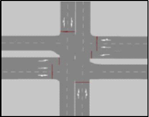
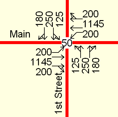
5.2 ARTERIAL BASE CONDITION ANALYSIS

As with the individual intersection, the analysis of arterial data depends on having a standard against which various parameters can be compared. This situation was modeled as the base condition. It was intended to reflect the average conditions at a typical urban arterial with three intersections on a four-lane roadway with left-turn pockets at the intersections as shown in figure 16 and figure 17. The objective of testing this arterial scenario was to determine the effect of demand changes, offset, and left-turn phase sequence on the number of conflicts.

Figure 16. Illustration. Three-intersection arterial.

Figure 17. Illustration. Detail of intersection in three-intersection arterial.

The base condition reflected a relatively high demand typical of a peak hour with V/C = 0.85. A cycle length of 50 s was determined to be optimal, based on Synchro™. This combination of intersection geometry and demand was intended to reflect a normal peak-period situation. The study used changes in demand and signal timing parameters to assess the impacts on safety. The base condition is the standard against which the effects of these changes were measured.

Each of the three intersections had the same geometric configuration as the isolated intersection. The spacing between the first and second intersection was 1,320 ft, and the spacing between the second and third intersection was 1,500 ft. The demand volume was selected to achieve a V/C ratio of 0.85 for both the main and side street movements. The left-turn phasing was lead, protected only. Signal timing was optimized using Synchro™. The cycle length was 50 s. As with the single-intersection simulations, conflicts were generated using SSAM.

The base condition is the average of six, 1-h simulations. This condition resulted in a total of 430 conflicts with 342 rear-end conflicts, 38 crossing conflicts, and 50 lane-change conflicts.

5.2.1 Changes in Arterial Demand Expressed as V/C Ratios

The first investigation was to determine the effects of a change in the V/C ratio. The demand conditions for the 50-s cycle (V/C = 0.85) are shown in figure 18, and the demand conditions for the 105-s cycle (V/C = 1.00) are shown in figure 19. The cycle length was optimized in Synchro™. The levels of service under the 50-s and 105-s cycle lengths were C and D, respectively. Also, under these optimized conditions, the average intersection delay was 25 s per vehicle for the 50-s cycle and 50 s per vehicle for the 105-s cycle.

Figure 18. Illustration. Demand volumes for 50-s cycle (vehicles per hour).

Figure 19. Illustration. Demand volumes for 105-s cycle (vehicles per hour).

The conflicts by type are shown in table 34. Two observations can be made from this table. First, there is a significant reduction in all types of conflicts when the cycle length is increased from 50 s to 105 s in spite of the fact that the demand volume increased. Second, the overall magnitude of the change in the number of conflicts (21 percent) is statistically significant.

Table 34. Arterial conflicts by type.

5.2.2 Effect of Changing Offsets on Conflicts

The next arterial investigation was the impact of changing an offset with a 50-s cycle and retaining the original lead-lead left-turn phase sequence. To do this, the offset at the second signal was adjusted in percentage of the optimum cycle length from -30 to +30 percent, in steps of 10 percent of the cycle length. The conflicts were calculated for each step. The results are shown in table 35.

Table 35. Conflicts under different offset conditions (50-s cycle length).

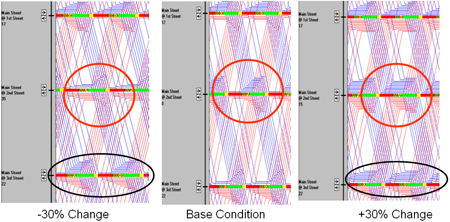
These results were unexpected. It was anticipated that as the offsets were adjusted away from optimum, more vehicles would have to stop and the number of conflicts would increase accordingly. This happened when the offset was increased but not when the offset was decreased. Moreover, the magnitude of the change in conflicts was much less than what might be expected. This is illustrated in the Synchro™ diagrams shown in figure 20.

Figure 20. Screenshot. Synchro™'s representation of flows impacted by offset changes.

Notice that there are much greater delays shown in the red circle in the illustration on the right compared to the delays depicted in the illustration on the left due to the queues that are predicted to build up in both directions of travel at the middle intersection. It is not known whether this phenomenon is a result of the specific geometry of the test network or a general fact that positive changes in offset have a more detrimental impact on queues and delays than negative changes to offsets. This phenomenon is important to consider for this research. Since this indicates that the changes to offsets have differential effects on efficiency, it might be reasonable to consider that changes to offsets could have differential effects on safety depending on the direction of adjustment.

To investigate this further, the simulations were repeated using the demand of V/C = 1.0 and a cycle length of 105 s. The results are shown on table 36.

Table 36. Conflicts under different offset conditions (105-s cycle length).

The first observation is that the number of rear-end conflicts with the optimum 105-s cycle is 288 while the number of conflicts with the 50-s cycle is 340, a 15 percent reduction by using a longer cycle length. The relative changes, with one exception, are similar in both instances, with the largest negative changes occurring when the offset is increased by 20 and 30 percent. A tentative conclusion is that the offset has little effect on conflicts until the change is more than +10 or -20 percent.

5.2.3 Effect of Left-Turn Phase Sequence on Conflicts

One additional signal timing parameter, left-turn phase sequence, was expected to have an impact on the number of conflicts. The base condition assumes that there is a lead left-turn phase in each direction on the main street. This is referred to as lead-lead phasing. One alternative that can be used to improve the flow on the arterial is to allow a lead left turn in one direction coupled with a lag left turn in the opposing direction. In both cases, the left-turn phase is protected only. This phasing strategy is only effective when the spacing between the intersections is uneven. In the test scenario, the difference between 1,320 and 1,500 ft is enough of a difference to impact the traffic flow.

As with the other test scenarios, the data were collected for both the 50-s cycle and the 105-s cycle. The results for the 50-s cycle (V/C = 0.85) with optimized offsets are shown in table 37.

Table 37. Arterial conflicts with lead-lag left-turn phasing (50-s cycle, V/C = 0.85)

This analysis suggests that the conflicts are proportional to demand as long as the through traffic has a progression window, which it had in this scenario by virtue of the lead-lag phasing. However, when compared to the lead-lead alternative, there is an increase in conflicts. The lead lead (V/C = 0.85) experienced only 430 conflicts compared to 504 with the lead-lag phasing—a 17 percent increase. A similar analysis was conducted for the 105-s cycle (V/C = 1.0), and the results are shown in table 38.

Table 38. Arterial conflicts with lead-lag left-turn phasing (105-s cycle, V/C=1.0).

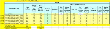
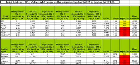
The results for the 105-s cycle are similar to the results of the 50-s cycle. There were 340 conflicts with lead-lead phasing. This was only 8 percent fewer than found with lead-lag phasing. As with all of the previous comparisons, the longer cycle length resulted in fewer conflicts—34 percent fewer in this case.

5.3 STATISTICAL TESTING AND CONFIDENCE IN THE RESULTS

5.3.1 Sample Size and Statistical Results from Multiple Simulations

Each test scenario for measuring the effect of signal timing on conflicts was simulated with multiple iterations, each using different random number seeds, and statistical distributions of the results were collected and analyzed. See figure 21 for a typical summary of results. Initially, a sample size of six simulation runs was selected. The frequency of each type of conflict was averaged and included a standard deviation and coefficient of variances. Subsequently, a sample size of 20 simulation runs was performed, and the results were averaged and compared to the average and statistical distribution for the set of 6 simulation runs. An F-test was performed (using 95 percent level of confidence and 10 percent standard error of the mean) to compare the statistical differences of the means. The results indicated no differences. Therefore, because of time and budget constraints, a sample size of six 1-hr simulations was selected for each test scenario in this project.

Figure 21. Screenshot. Typical summary of statistical distribution data.

5.3.2 Comparison of Base Condition Scenarios and Various Changes in Signal Timing Settings

Variations from the base scenario, such as a change in demand or a change in splits, were compared statistically to identify the significance of the difference from the base condition. The t-test was used to compare each surrogate measure of safety and the frequency of conflicts for various changes. The t-test calculated the probability of the difference of the two means. In this test, the null hypothesis (H0) indicated that the difference between the means of two samples is zero. Based on the difference level of the two sample variances, t-ratios and degree of freedom were calculated in different ways. Whether or not the sample variances were significantly different was verified by using the F-test before the t-test. When the average number of events in a conflict category and/or total conflicts was less than 0.5 (meaning that out of the 10 replications, an event occurs approximately every other simulation run), the data were marked as N/A, and no test outcome was recorded. An example of the t-test results is shown in figure 22.

Figure 22. Screenshot. An excerpt of t-test statistical output from SSAM.

5.4 SUMMARY OF SIMULATION STUDIES

The sequence of simulations was intended to identify which signal timing parameters had the most impact on conflicts. To do this, every attempt was made to isolate the impact of each parameter in subsequent tests. Several parameters were identified as having a strong association with conflicts, and several had less convincing associations. One parameter, cycle length, was identified as having a dominant association with conflicts. These results are summarized in table 39.

Table 39. Parameter-conflict association.

Several conclusions may be reached with high confidence based on these simulations. The findings are as follows:

• Cycle length is the dominant factor affecting the number of conflicts.

• Offsets and splits have a direct effect on safety.

• Left-turn phase protection and phase sequence have a significant effect on safety.

• All of these factors interact with one another.

This effort, so far, has only examined the single effect of individual signal timing parameters on conflicts and safety. The combined effect of aggregating multiple parameters with multiple intersection lane configurations was not tested. The next step of this research project must focus on these interactions to examine how these parameters affect each other and how combined changes can reduce the number of conflicts at signalized intersections without adversely affecting operational efficiency. Addressing these issues will require a carefully designed experiment and will provide the foundation for the algorithm development that will enable a real time adaptive control algorithm to balance safety and efficiency.

The next section of this report describes the experimental design approach for combining the effects of signal timing parameters and specifies the algorithms for combining safety and efficiency measures in a real-time adaptive control system.