• Federal Highway Administration >
• Publications >
• Research Publications >
• 98096 >
• Ch03.Cfm >
• Modeling Intersection Crash Counts and Traffic Volume - Final Report

Modeling Intersection Crash Counts and Traffic Volume - Final Report

3. THE DATA

3.1 Washtenaw County

3.2 California data

3.3 Minnesota data

3.4 Identifying unrealizable intersection approach volumes

3.1 Washtenaw County

Data from intersections in Washtenaw County, Michigan, were taken from a report by the Ann Arbor – Ypsilanti Urban Area Transportation Study Committee, Washtenaw County Intersection Crash Analysis, dated April 1991. It contains data for 134 signalized urban or suburban intersections consisting of traffic volumes on the crossing streets, and crash counts for each of the years 1986–89. Only intersections with 10 or more crashes in at least one year were included. This biases the models derived from the data, and the findings should be interpreted with caution. In a few cases, data were not available for all four years. These counts were expanded by the appropriate factor to estimate a total for the four years.

A careful inspection of the traffic volumes showed that they often remained constant over several adjacent intersections on the same road. While it may be the case that traffic volume varies little over longer stretches of certain roads, this has to be established. Simply carrying data from counting sites over several intersections not only biases the traffic volumes used, but also introduces a correlation between the errors of the volumes of these intersections. This invalidates error estimates obtained by standard statistical methods.

Despite the limitations, the Washtenaw County data were studied because they were readily available early during the study.

Top

3.2 California data

Data for the four–leg signalized urban intersections in California were those used by the Mid–West Research Institute in its study, Statistical Models of At–grade Intersection Crashes, by K.M. Bauer and D.W. Harwood. The data were not modified or processed in any way.

Top

3.3 Minnesota data

Minnesota data were obtained from the Highway Information System (HSIS) files. The Highway Safety Research Center of the University of North Carolina prepared the following files from the complete data set:

• An intersection route file, which contained one record for each route passing through a given intersection. This record contained information for both the incoming and outgoing legs. It also contained an intersection identification number that allowed matching with the record of the other route crossing the same intersection.

• A segment file, which contained cross–section data for each leg of each intersection. Legs were eliminated if they contained an extra intersection, including interchanges, grade crossings, etc. This was done to ensure that crashes linked with the legs are not related to any other intersection or interchange.

• A crash file, which contained records for all crashes anywhere on the legs retained, and corresponding vehicle and occupant files. Crash data for the year 1993 were used.

Route and segment files were processed to combine all data pertaining to a specific intersection into one record. Data for a total of 3,288 four–leg intersections were obtained. After selecting signal–controlled urban intersections that had volume information for all four legs, 71 intersections remained. Volume information was coded on both the route and segment files. The route file contained values of annual average daily traffic (AADT) for each of the two legs for up to five years. The segment file contained one value of AADT and the calendar year to which it pertained. Review of these values showed that the information on the route file was often old or incomplete. Therefore, information from the segment file was used when available. Otherwise volume information from the route file was used.

A review of the volume data showed that the same values of volume were often carried over long distances and over several intersections. Furthermore, often the four volumes were so different that it appeared questionable whether they could result from physical maneuvers. Therefore, the analysis described in the next section was performed.

Top

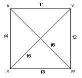
3.4 Identifying unrealizable intersection approach volumes

AADT values for all legs of many intersections were available in the Minnesota HSIS file. The question arose: Could all the given values have arisen from real traffic flows?

As an example, we considered an intersection with the AADT values 13247, 13247, 9488, and 13046 vehicles per day (vpd), shown in Figure 3A.1. At first glance it appeared questionable whether these values could have resulted from actual traffic: 13247 vpd would have been the traffic between the first and second leg, 9488 vpd could have been traffic from the third to the fourth leg, leaving 3556 vpd on the fourth leg, which could be explained only by 1779 vpd entering the intersection from the fourth leg, making a U–turn in the intersection, and leaving it on the fourth leg. This pattern is shown in Figure 3A.2 and is very implausible.

A slightly more complex traffic pattern, shown in Figure 3A.3, could explain the observed volume values. We assumed that 9488 vpd is the through traffic between the third and fourth leg. We interpreted the remaining volume of 3556 vpd on the fourth leg as a flow of 1778 vpd between the first and the fourth legs, and a flow of 1778 vpd between the second and fourth legs. A flow of 11469 vpd = 13247 vpd –1778 vpd between the first and the second leg completed the pattern. Thus, the observed volume values could have originated from actual traffic, though the actual traffic pattern is likely to be different from that used to demonstrate the feasibility.

Since it is not always obvious when a combination of volumes is realizable, a simple mathematical test was derived. We assume that only total volumes, without distinguishing directions are given, that no legs are one–way, and that there are no turn restrictions. It also is possible to derive tests for such conditions, but they would be more complicated.

Figure 3 shows the flows we distinguish at a four–leg intersection. They must add up to the volumes u, v, w, and x on the legs:

• f₁ +f₄+f₅ = u    (3-1)

• f₁+f₂ +f₅ = v    (3-2)

• f₂+f₃ +f₆ = w    (3-3)

• f₃+f₄ +f₆ = x    (3-4)

Figure 3. Flows distinguished at an intersection.

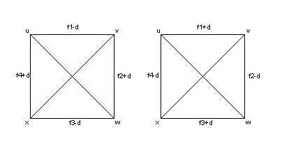
For the four volumes u, v, w, and x to be realizable by actual traffic flows, the system of equations (3–1) through (3–4) must be solvable by nonnegative values f _i , (i = 1, 2, ..,6).

To derive a condition for that, we represent the pattern of Figure 3 in a different manner in Figure 4. We assume that a realizable solution exists, and that x is the smallest of the four volumes.

Figure 4. Different representation of the traffic flows shown in Figure 3. (Not available)

Figure 5 shows how the flows f₁...f₄ can be changed, so that a realizable solution remains. One can choose d so large that either f₁–d or f₃–d becomes zero, or that either f₄–d or f₁–d becomes zero. Since x was assumed to be the smallest of the four volumes, it can be shown that either f₃–d=0, or f₄–d=0 can be obtained. This gives a new flow pattern.

Figure 5. Deriving other relizable solutions from a given realizeable solution, d is the value by which the original flows are changed.

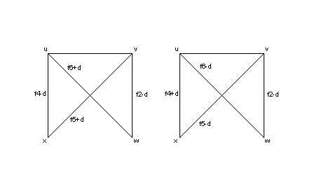
The case where f₃ is reduced to zero is shown in Figure 6.

Figure 6. A new flow pattern, resulting from a modification shown in Figure 5, and possible further modifications of the flow pattern.

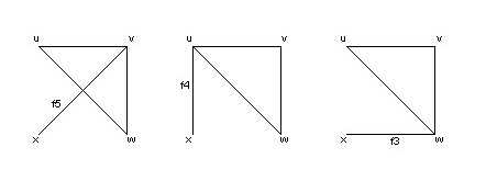
Again, the new flow pattern can be changed by adding and subtracting the same amount d to certain flows. This results in reducing f₄-d or f₅-d to zero, again because x is defined to be the lowest or one of the lowest volumes. Similarly, the other modifications of Figure 5 can be modified. All possible resulting flow patterns are shown in Figure 7.

Figure 7. The simplest flow patterns obtainable if x is a minimal volume on the legs.

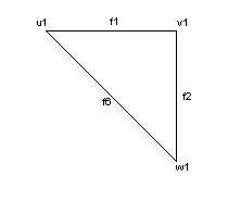
These three patterns can be transformed into a single pattern. In the first case, one sets f₅=x, and replaces u by u₁=v=x. In the second case, one sets f₄=x and replaces u by u¹=u=x, and in the third case one sets f₃=x and replaces u by w¹=w-x Thus, all three cases can be represented by the simple problems shown in Figure 8, where one of the u¹,v¹,w¹ is the modified one, and the other two have the original values.

Figure 8. Reduced flow pattern to derive conditions for reliability of leg volumes.

The conditions to be satisfied are:

• f₁ +f₆= u¹    (3-5)

• f₁+f₂ = v¹    (3-6)

• f₂+ f₆ = w ¹    (3-7)

If they can be satisfied by nonnegative values f₁,f₂ and f₆, the original u, v, w, and x can result from real traffic flows. To obtain conditions for satisfying conditions (3-5)...(3-7) with nonnegative numbers, we solve for f₁,f₂, and f₆.

• 2f₁ = u¹+v¹-w¹    (3-8)

• 2f₂ = u¹+v¹-w¹    (3-9)

• 2f₆ = u¹+v¹-w¹    (3-10)

Since the f₁ must be nonnegative, we have the conditions

• u¹+v¹-w¹ ³ 0    (3-11)

• -u¹+v¹+w¹ ³ 0    (3-12)

• u¹-v¹+w¹ ³ 0    (3-13)

The u¹,v¹,w¹ could have originated in three ways: by subtracting x from u, from v, or from w. Thus, we actually have three sets of conditions:

• u+v-w ³ x    (3-14)

• -u+v+w ³ -x    (3-15)

• u-v+w ³ x    (3-16)

or

• u+v-w ³ x    (3-17)

• -u+v+w ³ x    (3-18)

• u-v+w ³ -x    (3-19)

or

• u+v-w ³ -x    (3-20)

• -u+v+w ³ x    (3-21)

• u-v+w ³ x    (3-22)

only one of which needs to be satisfied to ensure realizability of u, v, w, and x. It is possible to rename the variables so that

• u ³ v³ w ³ x    (3-23)

Then, u+v ³ w+x holds. Therefore conditions (3–14) and (3–17) are satisfied, and since w+x ³ –v, condition (3–20) also is satisfied. Since u+w ³ v+x, conditions (3–16) and (3–22) hold, and because v+x ³ v–x, condition (3–19) is satisfied. What remains is that one of the conditions (3–15), (3–18), or (3–21) must be satisfied. Since the last two are identical,

• v+w ³ u-x    (3-24)

and

• v+w ³ u+x    (3-25)

remain. It is sufficient that one of the two is satisfied. If condition (3–24) is satisfied, a realizable flow pattern exists. If condition (3–24) is not satisfied, then condition (3–25) cannot be satisfied. Thus, the only effective condition for reliability of volume by flow patterns is that

• v+w+x ³ u    (3-26)

or that the largest volume on a leg must not be larger than the sum of the other three volumes.

The condition for realizable traffic volumes for three–leg intersections, obtained in the same manner, requires that the largest volume cannot be larger than the sum of the two smaller volumes.

The test was applied to four–leg intersections in the Minnesota data file. For signalized intersections, no unrealizable volume combinations were found. Among the 139 urban stop–controlled intersections with complete volume information, 2, or 1.4 percent had unrealizable volume combinations. Among the 438 rural stop–controlled intersections, 17, or 3.9 percent had unrealizable volume combinations. The data for these intersections are shown in Tables 3.4–1 and 3.4–2.

A closer look at the tables shows that, in some cases, condition (3–26) is nearly satisfied, whereas in others the discrepancy is very large. If the AADT values were obtained from a single 24–hour count, a plausible first approximation is to assume them to be Poisson – distribution, for which an estimate of the variance is equal to the actual count. If a seasonal adjustment factor is applied, its square must be applied to the variance of the actual count. If the AADT is calculated from the average of n 24–hour counts, then its variance is reduced by a factor of n compared with that obtained by a single 24 hour count. Therefore, without knowing the seasonal factor and the number of days of counting, we cannot realistically estimate the variance resulting from the random character of traffic. However, if one is willing to use the Poisson assumption for estimating the standard errors of an AADT figure, one can make some comparisons. In Table 3.4–1, the discrepancies are four and six times the standard deviation, which is too much to be acceptable as resulting from random variability.

In Table 3.4–2, the discrepancies range from 0.2 to 128 times the assumed standard deviation. In five cases the discrepancies are less than twice the assumed standard deviation, indicating that least some of them may be due to random fluctuations of the traffic count. However, in the remaining 12 cases, the discrepancies are unlikely to have resulted from random variations.

Top

FHWA-RD-98-096