A Safety Evaluation of UVA Vehicle Headlights
CHAPTER 3
Cost/Benefit Analysis
INTRODUCTION
The field evaluation of ultraviolet (UVA) headlamps and fluorescent traffic control devices (TCDs) involved eight experimental procedures designed to determine the effectiveness of UVA technology. The procedures were conducted on a closed series of roadways and involved objective and subjective methods. The visibility of roadway delineation and staged roadway scenes depicting pedestrians, bicycles, and disabled vehicles was compared using standard U.S. headlights, European specification (ECE) headlights, and UVA headlights. This section will describe the experimental methodology in detail. The following topics will be addressed:
- Experimental Test Sites
- Testing Equipment
- Vehicles
- Windshield Shutter
- Lane Aligners
- Test Subjects
- Research Personnel
- Testing Procedures
- Roadway Delineation Visibility Study
- Static Pedestrian Visibility Studies
- Left-Curve Visibility Study - With and Without Glare
- Dynamic Pedestrian Visibility Study
- Disabled Vehicle Visibility Study
- Loop Ride Study - Subjective Ratings
- DASCAR Drive Study - Driver Performance and Subjective Ratings
- Static Testing - Visibility Distances and Subjective Ratings
- Results
- Detection and Recognition Distance
- Roadway Delineation
- Roadway Scenes
- Pedestrian Scenes
- Static Testing
- Driver Performance Measures-DASCAR
- Subjective Ratings
- Age Effects
EXPERIMENTAL TEST SITES
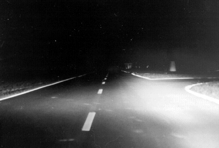
The various procedures were conducted at one of two sites located on the grounds of the Federal Bureau of Investigation (FBI) Training Academy driver training facility in Quantico, Virginia. New pavement-marking thermoplastic with UVA-activated fluorescent pigment and glass beads provided by Cleanosol were installed at both sites in November 1996. Testing began in May 1997 when the markings were about 6 months old. The layout of the roadways at both sites is shown in Figure 1.
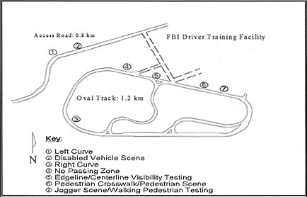
Figure 1. Test track layout.
The test track location consisted of a 1.6-km (1.1-mi) oval test track that was primarily a two-lane roadway. The pavement markings included white solid edge lines and double solid yellow center lines. The track widened to four lanes on the southern side of the course. There was no overhead lighting. On the northern side of the course and within the primary test track, there was a straight and level segment of roadway that was striped as a passing zone with a yellow dashed center line. A standard parallel pedestrian crosswalk was installed on the straight and level segment.
Fluorescent post-mounted delineators were installed on both sides of the curve on the northwest corner of the track. They were positioned 2.4 m (8 ft) from the paved roadway. The posts were made of heavy-duty plastic and appear yellow in daylight and fluorescent green under UVA light. The other three curves on the course did not have post-mounted delineators.
Near the middle of the test track a narrow reverse curve segment of roadway connected the north and south sides of the test track. Only white UVA-activated fluorescent edge line markings were installed on the reverse curve. Another connecting road with a blind curve was near the southeast corner of the track. This segment of roadway was also striped with white UVA-activated fluorescent paint edge lines.
The access road, located about 0.8 km (0.5 mi) from the test track, was 1.3 km (0.8 mi) in length and ended at a closed gate. White UVA-activated fluorescent edge lines and double solid yellow UVA-activated fluorescent center lines were installed. The access road had two unsigned curves and one sharp curve signed with an advisory curve turn arrow and marked for 32.3 km/h (20 mi/h). Guardrails were installed at a location near one of the unsigned curves. Guardrails with one amber reflector marker attached on each end were located near one of the unsigned curves. An unpaved gravel shoulder lined both sides of the roadway. There was no overhead lighting.
Six fluorescent post-mounted delineators were installed near the right lane on the outside of the left curve. They were positioned 1.2 m (4 ft) from the paved roadway. The advisory curve turn sign, previously installed in advance of the left curve, was covered with a black painted plywood cover during the Left Curve Delineation Visibility Study and the Disabled Vehicle Visibility Study and left uncovered during the DASCAR Drive Study.
TESTING EQUIPMENT
The testing equipment included two specially equipped research vehicles. Both vehicles were fitted with UVA headlight units from Ultralux, a windshield shutter, and a lane aligner. A third vehicle, also equipped with a lane aligner, was used to simulate the headlight glare from an oncoming vehicle.
Vehicles
One of the vehicles used was a 1994 Ford Taurus station wagon. The Taurus was equipped with the DASCAR (Data Acquisition System for Crash Avoidance Research) instrumentation package developed by the National Highway Traffic Safety Administration (NHTSA). DASCAR can record up to 33 experimental parameters. Driver inputs such as steering, braking and accelerator, and GPS (Global Positioning System) inputs are recorded at a rate of 30 data points per second by a hard drive located in the rear of the vehicle. In addition, four video cameras are available to record two views of the driver as well as front and rear view out of the vehicles. Because all of the testing was done at night and because both test sites had no overhead lighting, the video cameras were not used. Although DASCAR has the capability of recording 33 different parameters, not all of these were relevant to a study of headlight effectiveness. It was hypothesized that improved vehicle lighting might produce changes in driver lane tracking and speed selection. For this reason, the following parameters were used: vehicle speed, braking applications, steering inputs (amplitude and direction), and vehicle lateral placement in the traffic lane.
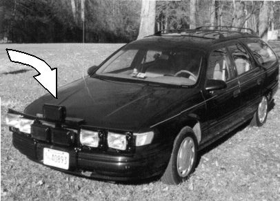
The Taurus was also equipped with a custom steel rack fabricated by Kropp Tool Co., Berlin, Pennsylvania, to support the headlight units. A total of seven headlight units were installed on this rack:
- 3 Ultralux UVA headlights,
- 2 U.S. specification headlights (H6054 sealed beams), and
- 2 European specification headlights (ECE with H-4 elements).
As shown in Figure 2, the UVA units were installed in a triangular configuration; two were just above the bumper in the center of the vehicle and the third was just above the lower two. The U.S. and ECE headlights were also installed just above the bumper along side the UVA units, in the same horizontal and vertical plane as the Taurus headlights. Since the test headlights were installed directly in front of the standard Taurus headlights, the standard Taurus headlights were not used. The U.S., ECE, and UVA headlights were controlled by switches mounted on the dash.
Figure 2. UVA headlight configuration on the Taurus test vehicle.
The Taurus was used for the driver performance testing and two of the static tests and the subjective ratings.
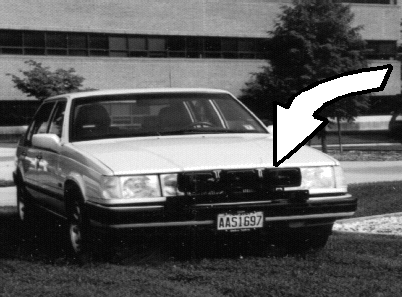
The second experimental vehicle was a 1993 Volvo 960. The Volvo also had three Ultralux UVA headlight units. These units were mounted on a steel framework in front of the grille and on top of the bumper. The configuration of the UVA lamps on the Volvo test vehicle is shown in Figure 3. This test vehicle is the same vehicle used in a previous FHWA study (Mahach, Knoblauch, Simmons, Nitzburg, Arens, and Tignor, 1997), and was leased from Volvo of America. The Volvo had Society of Automotive Engineers (SAE) specification composite headlight units with standard H-4 Halogen elements that were used for the standard U.S. low-beam testing condition. Like the Taurus, the Volvo was equipped with switches so that the UVA units could be activated from the cabin, independently of the regular headlights.
Figure 3. UVA headlight configuration on the Volvo test vehicle.
The Volvo was used for six of the static tests and the subjective rating procedure.
For all testing, the UVA headlight units were used as a supplement to either the U.S. or the European specification headlight. No testing was done with the UVA units alone. Throughout this report, "UVA" headlights will refer to the lighting conditions provided by two U.S. specification headlight sealed beams (H6054) and the three Ultralux supplemental UVA headlight units. In those testing situations where the UVA headlights were combined with the European specification headlights, the headlight condition will be described as Euro/UVA.
Two of the experimental procedures involved simulating glare from an oncoming vehicle. A 1990 Ford Tempo with standard composite U.S. headlights and H-4 elements was used for these procedures.
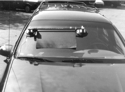
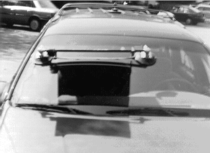
Windshield Shutter
The purpose of some of the field testing was to determine the effect of UVA headlights on the conspicuity of various visual stimuli at different distances. To do this, it is appropriate to limit the time available for visual search (Cole & Jenkins, 1980). This was done by using a windshield shutter to limit the exposure time of the subjects to the roadway scenes at each of the test distances. The shutter was a 304.8-mm by 533.4-mm (12-in by 21-in) flat panel that was lifted from the windshield surface by a rotational solenoid connected to a 12V power source. The shutter assembly was mounted on the outside of the passenger-side windshield with rubber suction cups. Photographs of the windshield shutter (closed position and open position) installed on the Taurus Test vehicle are shown in Figure 4. The shutter was positioned so that each subject could see a distance of 30 m (98.4 ft) in front of the vehicle when the shutter was closed. This 30-m (98.4-ft) distance allowed the subjects to retain their adaption to pavement luminance and reduced the amount of refocusing needed to detect the experimental stimuli. The experimenter controlled the shutter from the driver's seat by pushing a button that activated an adjustable timer controlling the amount of time the shutter was open. Based on previous human factors research and initial pilot testing, it was determined that a 2-sec stimulus exposure time was appropriate. The windshield shutter was used for six of the experiments.
Lane Aligner
In order to properly conduct the experiments, it was essential that the orientation of the test vehicles be the same in each trial. Having the vehicles' headlights pointing either to the left or to the right could seriously affect the conspicuity of the stimuli. In order to ensure an identical lane position from trial to trial, each vehicle was equipped with a lane aligner. The lane aligner was a custom-fabricated telescoping outrigger that was installed under the left side of both the front and rear of each vehicle. At the start of each testing session, the outriggers would be extended a predetermined distance from the side of each vehicle.
A small downward-facing light at the end of each outrigger could be activated by the experimenter. By positioning these lights directly over the center line of the roadway, the experimenter could consistently position the experimental vehicle within the travel lane in each trial.
Down or Closed Position
Up or Open Position
Figure 4. Windshield shutter installed on the Taurus test vehicle.
TEST SUBJECTS
Subjects were recruited from the northern and central Virginia regions through classified ads in local papers. Several prescreening meetings were held at local hotels and community centers. Each potential subject was given a test for visual acuity and color vision. A questionnaire was administered that included a self-assessment of driving abilities, day and night driving frequency, questions about headlight glare, and a general biographical inventory. After presenting a valid U.S. driver's license, subjects read the informed consent form and were scheduled for participation.
A total of 38 subjects ranging in age from 18 to 76 were tested. The mean age was 40.5 years. Ten of the subjects were age 55 years or older. A discussion of age effects is included in a later section. There were 16 males and 22 females. Two subjects were tested each evening, starting when it became dark. Testing typically started between 9:00 p.m. and 9:30 p.m. and concluded between 11:30 p.m. and midnight. Because access to the test facility was limited to two evenings per week, only four subjects per week could be tested. The field effort began in May 1997 and concluded in August 1997.
RESEARCH PERSONNEL
Two research teams, consisting of two individuals each, conducted all nine of the experiments. Each team was responsible for all of the experiments that were conducted at one of the two sites. The team that used the Volvo conducted five of the experiments, and the team that used DASCAR conducted four of the experiments.
Each experimenter had their own responsibilities that remained constant from night to night. Certain experimenters worked directly with the subjects and others recorded data, controlled the headlight glare vehicle, set the roadway scenes, and served as the staged walking pedestrian.
The experiments were designed so that each team tested one of two subjects for 75 minutes. After a 15-minute break, the subjects switched locations (and teams) and some of the same experiments were repeated. Half of all the subjects took part in the Dynamic Pedestrian Visibility Study and half took part in the Disabled Vehicle Visibility study. This schedule was necessary because some of the experiments were more time-consuming than others.
TESTING PROCEDURES
Nine distinct research procedures were designed to assess the effectiveness of UVA lighting and fluorescent traffic control devices. The procedures determined detection distances, recognition distances, and subjective ratings, as well as driver performance measures. Each of the following research procedures will be described:
- Roadway Delineation Visibility Study
- Static Pedestrian Visibility Study
- Left-Curve-Visibility Study - With and Without Glare
- Dynamic Pedestrian Visibility Study
- Disabled Vehicle Visibility Study
- Loop Ride Study - Subjective Ratings
- DASCAR Drive Study - Driver Performance and Subjective Ratings
- Static Testing - Visibility Distances and Subjective Ratings
Roadway Delineation Visibility Study
The roadway delineation visibility tests were conducted with the subject in the right front passenger seat of the Volvo. During pilot testing, the point where each target stimuli could not be seen using any of the test headlights was determined. This location served as the first station for each of the testing scenarios. Starting at the first station, the experimenter moved progressively closer to the stimulus, stopping at stations every 30.5 m (100 ft). The subjects were told that they were looking for a specific stimulus—either the end of a no-passing zone, a right curve, or a crosswalk. At each station, the subject was asked to indicate whether he or she "can't" see the stimulus, "thinks" he or she sees the stimulus, or is "absolutely sure" that he or she sees the stimulus. The windshield shutter was used to limit the subject's visual exposure to the stimulus to 2 sec. Headlight conditions tested were U.S. and UVA. Three pavement marking conditions on the oval test track were used as stimuli. A no-passing zone was located at the end of the long tangent section on the north side of the track. The first station was 274.5 m (900 ft) from the start of the double yellow lines. The right curve was located on the southwest corner of the track. The first station was 335.5 m (1,100 ft) from the start of the curve. The crosswalk was located on the tangent section on the north side of the track. The first station was 274.5 m (900 ft) from the crosswalk. The order of presentation of the headlight condition was counterbalanced. A second observer in the backseat recorded the subject's responses on a data collection form.
Static Pedestrian Visibility Studies (Two Scenes)
These static tests used a procedure similar to the Roadway Delineation Visibility Study. Subjects, starting beyond the point where the stimuli were visible, were moved progressively closer in 30.5-m (100-ft) intervals. When the windshield shutter was raised, they were instructed to indicate what they thought they could see and, when they were more certain, what they were sure they could see. Their responses were tape recorded. The tapes were transcribed and coded. Coding criteria were developed so that responses could be categorized as "I think I see..." and "I'm sure I see..." for each of the target stimuli. The subjects were given no indication as to the type of stimuli being presented.
Distances at which subjects indicated that they thought they saw something were tabulated as the detection distances. Distances at which subjects indicated they were sure they saw a specific stimuli were tabulated as recognition distances.
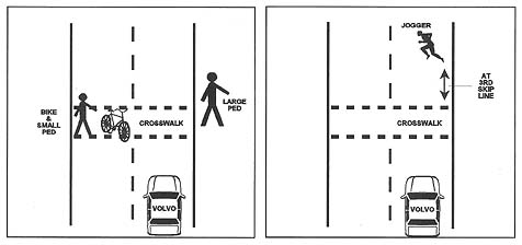
Two different roadway scenes were set up on the tangent section of the oval track. The layout of the two scenes is shown in Figure 5. Life-size silhouettes of pedestrians were cut out of 6-mm-thick (¼-in-thick) plywood. The pedestrian dummies were clothed in garments that had been washed once in a commonly used laundry detergent. The pedestrian dummies were used to create two different roadway scenes. The first scene consisted of a small child in a lavender skirt and a 51-cm (20-in) child's bicycle (painted with fluorescent yellowish-green spray paint) in the left lane. A second adult-size pedestrian cutout wearing khaki pants and a medium- to light-colored polyester shirt was located on the right edge line. Both cutouts were in the crosswalk. The second scene had a pedestrian cutout, with a light-grey cotton shirt and shorts, in the right lane approximately 20 m (65.6 ft) beyond the crosswalk. The pedestrian cutout appeared to be jogging across the roadway. The order of presentation of the two headlight conditions were counterbalanced.
Left-Curve Delineation Visibility Study (With and Without Oncoming Headlight Glare)
This study was a static test of the visibility distance of a left curve in the roadway. Like some of the previous tests, the vehicle, with the subject in the right front passenger seat, moved progressively closer to the stimuli in 30.4-m (100-ft) intervals until it was positively identified. The Taurus, with the windshield shutter in position, served as the test vehicle. The Tempo, driven by the second experimenter, was positioned in the opposing lane 60.8 m (200 ft) in front of the test vehicle with the headlights (low beams) turned on to simulate oncoming headlight glare. Two orders of presentation of headlight condition (U.S. or UVA) were used, first without oncoming headlight glare and then with oncoming headlight glare. Unlike some of the previous tests, the subjects were told that they were looking for a left curve in the road ahead. Hence, no detection distance measures were taken and only a recognition distance measure is reported in the results section. They were simply asked if they could see the left curve ahead when the windshield shutter was raised. Their responses were tape recorded.
|
PEDESTRIAN/BIKE SCENE |
JOGGER SCENE |
DISABLED VEHICLE SCENE
Figure 5. Stimulus configurations: static pedestrian
visibility studies and disabled vehicle visibility study.
Dynamic Pedestrian Visibility Study
This study used a procedure similar to that used for the Static Pedestrian Visibility Studies; however, the stimuli and the subject response codes were different. Because a moving pedestrian (especially with the UVA headlights on) is very easy to recognize, it was decided to create a more challenging visual task—one involving headlight glare from a stationary oncoming vehicle. The 1990 Ford Tempo was positioned in the approaching (left) travel lane with the low-beam headlights on. On cue from the experimenter in the Volvo, a second experimenter (wearing light upper clothing and jeans) began walking across the right lane 10 m (30 ft) to the rear of the Tempo and directly in front of the subjects in the test vehicle. The windshield shutter was raised and the subject indicated whether or not he saw a pedestrian. The subjects were instructed to respond in one of three ways:
- Did not see a pedestrian,
- Thought I saw a pedestrian, or
- Absolutely sure I saw a pedestrian.
There were two trials at each station; one where there was a pedestrian and one where there was no pedestrian. The order of presentation of the stimulus (pedestrian or no pedestrian) was counterbalanced. All subjects were first tested with the U.S. headlights, followed by the UVA headlights.
Disabled Vehicle Visibility Study
This study was a static test of the visibility of a disabled vehicle scene. The test subject was in the right front passenger seat of the Taurus with the windshield shutter in position. A disabled vehicle roadway scene was created using a parked vehicle (1995 blue Toyota Celica, with the reflective license plate covered) on the shoulder of the opposing lane. The layout of the disabled vehicle scene is shown in Figure 5. A plywood cutout of a kneeling pedestrian, wearing pants and a white long-sleeved shirt, was located near the vehicle's left rear tire. A second plywood cutout of an adult pedestrian, wearing dark navy-colored pants and a medium dark blue shirt, was located 2.1 m (7 ft) in front of the disabled vehicle and 152 mm (6 in) to the outside of the left edge line. In addition, two orange fluorescent traffic cones, measuring 0.6 m (2 ft) in height, were located near the kneeling pedestrian and the left rear tire. The subjects were asked to indicate what they could see when the windshield shutter was raised. Their responses were tape recorded. The tapes were transcribed and coded. Responses were categorized to identify detection ("I can see something") and recognition ("I can see a car and people") distances.
Loop Ride Study - Subjective Ratings
The loop ride was a dynamic test with the subject riding in the right front passenger seat of the Volvo. Site 1, the 1.6-km (1.1-mi) oval test track, was used. The procedure began with one experimenter reading the script that instructs the subjects to observe the roadway markings and headlights and provide subjective comparisons with what they generally see when driving at night. The subjects were first given an acclimation loop, always with the U.S. headlights. They were then driven on two additional loops with the U.S. headlights and the UVA headlights. Two different orders of presentation were used: U.S./UVA and UVA/U.S. After the second and third loops, the subjects were also asked to provide subjective comparisons with the headlights used in the previous loop. A second researcher, riding in the back seat, recorded the subjects' responses.
DASCAR Drive Study - Driver Performance and Subjective Ratings
During the DASCAR Drive Study, the subjects drove the Taurus with the DASCAR instrumentation package on five round trips of the access road (Site 2). The access road consisted of two straight tangent sections, two right curves, and two left curves. After a short period of time in order to become acclimated to the vehicle and to adjust the seat, controls, mirrors, etc., the subjects were given a brief description of the course. They were told that there would be an oncoming car driven by a research team member. They were told that the road was closed to all other traffic. They were told that after each run, they would be asked two questions about the headlights and the roadway markings. They were told to drive at a safe and comfortable speed, but not to exceed 48 km/h (30 mi/h). They were not told that the vehicle was fully instrumented and would be recording their driving behavior. Each subject made five round trips or loops. The first loop was described as a practice run and all subjects made the loop using U.S. low-beam headlights. Four additional loops were made using four different headlight conditions: Euro low beams; Euro low beams with UVA; U.S. low beams; and U.S. low beams with UVA. The stationary Ford Tempo with low-beam headlights was positioned using the lane aligner in the oncoming lane, on the tangent section in the middle of the loop. The Tempo was kept out of sight and moved into position just prior to the subject's return drive through the tangent section. At the end of each loop, the subject was told to stop the vehicle and was asked the following:
- How well did the headlights and roadway markings work for you compared to what you generally see when you drive your car? Response choices were: (a) not as good as; (b) as good as; or (c) better than.
-
And, on the second and subsequent loops:
- Compared to the last ride down to the gate and back, how well did these headlights and roadway markings work for helping you see where to steer the car? Response choices were: (a) not as good as; (b) as good as; or (c) better than.
Static Testing - Visibility Distances and Subjective Ratings
This procedure was a replication of tests conducted on the Clara Barton Parkway (near Washington, DC) in 1996 that was described in Mahach, Knoblauch, Simmons, Nitzburg, Arens, and Tignor (1997).
The Clara Barton procedure was a static test with the subject sitting in the right front passenger seat. No windshield shutter was used. The experimenter parked the Volvo, using the lane aligner, at a fixed point on the straight two-lane section of Site 1. Traffic cones with reflective collars were set up at 50-m (150-ft) intervals, 3 m (9 ft) to the right of the right edge line. The first part of the testing always used the U.S. headlights. The subjects were asked:
- How many centerline skip marks (dashed lines) they could count.
- How far they could see the right edge line (using the traffic cones as a point of reference).
- To rate (on a five-point scale) the overall visibility of the roadway markings.
The UVA headlights were then turned on and the subject was asked the same three questions. The experimenter recorded the subjects responses on a data form using a low-intensity penlight for illumination.
RESULTS
As previously described, the field study used a variety of experimental procedures to quantify the effectiveness of UVA/fluorescent technology. The results of the field study will be presented in this section. The discussion will be organized according to the measure of effectiveness (MOE) that was quantified. The following will be discussed:
- Detection and Recognition Distance
- Roadway Delineation
- Roadway Scenes
- Pedestrian Scenes
- Static Testing
- Visibility Distances
- Subjective Ratings
- Driver Performance Measures - DASCAR
Detection and Recognition Distance
Detection and recognition distances were measured using static testing scenarios in which the subject was moved progressively closer to the stimuli and a windshield shutter was used to limit exposure time. The results are being presented according to the nature of the stimuli. Three categories of stimuli will be discussed:
- Roadway Delineation
- Roadway Scenes
- Pedestrian Scenes
Roadway Delineation
Detection distance measuring procedures were developed for three different types of roadway delineation: right curve, start of a no-passing zone, and a pedestrian crosswalk. In these procedures, detection distance was defined as the point where the subjects indicated that they thought they could see the specific target ahead, but could not positively identify it as such (e.g., "I think I can see the crosswalk").
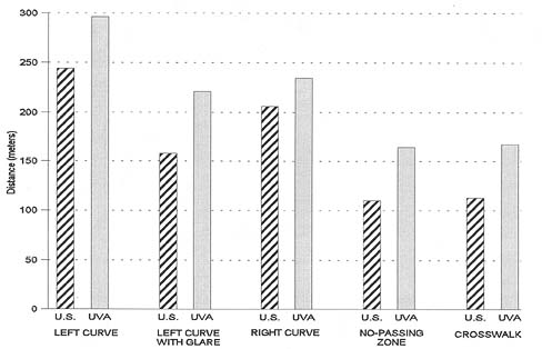
The results of the detection distance measuring procedures for the roadway delineation scenes are shown in Figure 6.
The UVA headlights outperformed the U.S. headlights for all roadway delineation scenarios. The percentage of improvement ranged from 53.6 percent for the pedestrian crosswalk to 32.3 percent for the no-passing zone to 6.1 percent for the right turn. While the differences for both the crosswalk and the no-passing zone were highly significant (0.000), the results for the right curve were not quite significant (0.074). The right-curve scene was on a slight downhill section that resulted in very long—more than 213.5 m (700 ft)—detection distances for both the UVA and the U.S. headlights and the UVA headlights appeared to offer somewhat less of an advantage in that situation.
| |
Right Curve |
|
No-Passing Zone |
|
Crosswalk |
| U.S. |
UVA |
U.S. |
UVA |
U.S. |
UVA |
| Mean |
228.3 |
242.2 |
148.8 |
196.9 |
129.4 |
198.7 |
| No. |
33 |
33 |
33 |
33 |
33 |
33 |
| Std. Dev. |
57.1 |
36.5 |
49.3 |
45.2 |
38.9 |
41.1 |
| t |
-1.844 |
-4.881 |
-9.193 |
| Signif. |
0.074 |
0.000 |
0.000 |
Figure 6. Roadway delineation — detection distances.
In these procedures, recognition distances were defined as the point where the subjects were "absolutely sure" that they could see the target stimulus (see p. 21). The results of these recognition distance measurements are shown in Figure 7. The percentage of improvement was computed by dividing the increase in recognition distance associated with the UVA headlights by the recognition distance associated with the U.S. headlights. The percentage of improvement in recognition distances with UVA headlights are as follows:
| Delineation |
Percent Improvement |
No-Passing Zone Crosswalk
Left Curve, With Glare
Left Curve, No Glare
Right Curve |
48.4%
48.4%
40.0%
21.4%
13.9% |
All of these differences were significant at the 0.001 level or better. It should be noted that the left-curve scene was not included in the previous discussion of detection distances because the experimental protocol limited the subjects to a simple "yes" or "no" response. They were not instructed to indicate when they "thought" they saw the stimulus as was the case with the procedure used for the no-passing zone, the crosswalk, and the right turn. It should be noted that in the left-curve visibility test, the UVA headlights were more effective when glare from an oncoming vehicle was present (40.0 percent) than when no such glare was present (21.4 percent).
| |
Left Curve |
Left Curve With Glare |
Right Curve |
No-Passing Zone |
Crosswalk |
| U.S. |
UVA |
U.S. |
UVA |
U.S. |
UVA |
U.S. |
UVA |
U.S. |
UVA |
| Mean |
244.0 |
296.3 |
157.9 |
221.1 |
206.1 |
234.8 |
110.0 |
164.5 |
112.8 |
167.3 |
| No. |
28 |
28 |
28 |
28 |
33 |
33 |
33 |
33 |
33 |
33 |
| Std. Dev. |
65.9 |
41.4 |
124.0 |
74.5 |
55.0 |
33.7 |
29.0 |
44.0 |
34.5 |
39.7 |
| t |
-5.645 |
-3.533 |
-3.881 |
7.408 |
-8.807 |
| Signif. |
0.000 |
0.001 |
0.000 |
0.000 |
0.000 |
Figure 7. Roadway delineation — recognition distances.
Roadway Scenes
Detection distances were determined for the following roadway scenes: a disabled vehicle, a fluorescent bicycle, and fluorescent traffic cones. The results of the detection distance measurements ("I think I see a ___") are shown in Figure 8. Visibility improvements with the UVA lighting are very impressive. The percentage of improvements for the three scenes are:
| Scene |
Percent Improvement |
Disabled Vehicle
Bicycle
Traffic Cones |
27.1%
283.6%
372.7% |
Although these improvements are very dramatic, it should be noted that both the bicycle and the traffic cones did not have a retroreflective component. The differences between U.S. and UVA headlights were significant for both the bicycle and the traffic cones, but not for the disabled vehicle. This is possibly because of the intrinsic differences between the test scenes. Both the bicycle (part of one of the pedestrian scenes with the child pedestrian) and the traffic cones (part of the disabled vehicle scene) were fluorescent and, therefore, detectable at relatively long distances with the UVA headlights. Except for the fluorescent traffic cones, the disabled vehicle scene was created to be a worse-case scenario. The disabled vehicle was dark colored with no fluorescent or retroreflective component. The tall standing pedestrian cutout had very dark clothing, making it difficult to see. Only the squatting pedestrian had a light-colored shirt that provided some visual cues to the subject relative to shape and positioning. In addition, given that the visual exposure was limited by the windshield shutter, the subject may not have had enough time to focus on both the fluorescent traffic cones and the disabled scene components. The detection distance differences demonstrate that UVA/fluorescent technology does not work as well in some situations as it does in others.
Pedestrian Scenes
Recognition distances were determined for the same three roadway scenes as well as the dynamic walking pedestrian scenario. Since the protocol restricted subjects to "pedestrian" or "no pedestrian" responses, only recognition distance measurements were reported for the walking pedestrian scenario.
| |
Disabled Vehicle |
|
Bicycle |
|
Traffic Cones |
| U.S. |
UVA |
U.S. |
UVA |
U.S. |
UVA |
| Mean |
164.2 |
120.0 |
62.0 |
237.9 |
25.8 |
122.0 |
| No. |
13 |
13 |
30 |
30 |
13 |
13 |
| Std. Dev. |
77.3 |
70.9 |
42.0 |
37.9 |
58.2 |
68.3 |
| t |
1.536 |
-18.857 |
-4.306 |
| Signif. |
0.150 |
0.000 |
0.001 |
Figure 8. Roadway scenes — detection distances.
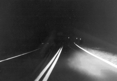
Improvements in recognition distances were very dramatic in three of the four scenarios (Figure 9). The walking pedestrian was visible at 152.5 m (500.00 ft) with the UVA headlights and only at 610 m (200.00 ft) with the U.S. headlights—a 150-percent increase. The fluorescent bicycle was recognizable at 123.02 m (403.33 ft) with the UVA headlights and at 38.63 m (126.67 ft) with U.S. headlights—a 218.4-percent improvement. The fluorescent traffic cones were recognizable at 91.50 m (300.00 ft) with UVA headlights and at 11.73 m (38.46 ft) with U.S. headlights—a very dramatic 679.7-percent improvement. All three of these differences were very significant (0.000 level). Although the more visually complex disabled vehicle scene was recognized 32.84 m (107.69 ft) sooner with the U.S. headlights compared to the UVA headlights, this 29.8-percent increase was not statistically significant. Photographs of the disabled vehicle scene illuminated by regular low beams and by regular low beams and UVA headlights are shown in Figure 10.
Detection and recognition distances were determined for five different pedestrian cutouts. As shown in Figure 11, improvement in detection distances with the UVA headlights ranged from 20.33 m to 139.88 m (66.66 ft to 458.62 ft). The percentage of improvement varied from 33.64 percent to 117.18 percent. Four of the five differences were significant at the 0.004 level or better. Figure 12 depicts the recognition distances for the pedestrian scenes. Again, four of the five pedestrian cutouts were seen for significantly greater distances with the UVA headlights. These distances were for 15.25 m (50.00 ft) to 58.89 m (193.08 ft) more and represent a 37.50-percent to 67.87-percent improvement. Photographs of one of the pedestrian scenes illuminated by regular low beams and UVA headlights are shown in Figure 13.
The fluorescent painted bicycle was so highly visible with the UVA headlights that the subjects may have been distracted by its presence long after they positively identified it as a bicycle. The high visibility of the bicycle in the scene may have distracted from the other objects in the scene—specifically, the child pedestrian that was located nearby. This would explain the relatively short detection and recognition distances reported for the child pedestrian.
| |
Disabled Vehicle |
Walking Pedestrian |
Bicycle |
Traffic Cones |
| U.S. |
UVA |
U.S. |
UVA |
U.S. |
UVA |
U.S. |
UVA |
| Mean |
143.1 |
110.3 |
61.0 |
152.5 |
38.6 |
123.0 |
11.7 |
91.5 |
| No. |
13 |
13 |
15 |
15 |
30 |
30 |
13 |
13 |
| Std. Dev. |
71.9 |
65.3 |
23.1 |
36.5 |
15.9 |
42.0 |
15.5 |
57.1 |
| t |
1.244 |
-7.685 |
-9.942 |
-5.226 |
| Signif. |
0.237 |
0.000 |
0.000 |
0.000 |
Figure 9. Roadway scenes — recognition distances.
Standard U.S. Low Beams
Standard U.S. Low Beams With UVA
Figure 10. Disabled vehicle scene shown with standard U.S. low beams
(above) and standard U.S. low beams with UVA (below).
| |
Child Pedestrian |
Adult Pedestrian |
Tall Pedestrian |
Kneeling
Pedestrian |
Jogger Pedestrian |
| U.S. |
UVA |
U.S. |
UVA |
U.S. |
UVA |
U.S. |
UVA |
U.S. |
UVA |
| Mean |
41.7 |
62.0 |
111.8 |
149.5 |
103.2 |
178.3 |
112.6 |
164.2 |
119.4 |
259.3 |
| No. |
30 |
30 |
30 |
30 |
13 |
13 |
13 |
13 |
29 |
29 |
| Std. Dev. |
17.0 |
31.5 |
41.9 |
51.5 |
52.1 |
58.2 |
51.9 |
73.2 |
39.5 |
39.1 |
| t |
-3.162 |
-3.479 |
-4.064 |
-1.821 |
-19.474 |
| Signif. |
0.004 |
0.002 |
0.002 |
0.094 |
0.000 |
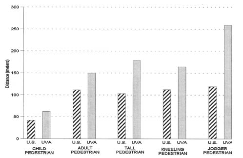
Figure 11. Pedestrian scenes — detection distances.
| |
Child Pedestrian |
Adult Pedestrian |
Tall Pedestrian |
Kneeling Pedestrian |
Jogger Pedestrian |
| U.S. |
UVA |
U.S. |
UVA |
U.S. |
UVA |
U.S. |
UVA |
U.S. |
UVA |
| Mean |
40.7 |
55.9 |
76.3 |
114.9 |
91.5 |
129.0 |
93.8 |
105.6 |
86.8 |
145.7 |
| No. |
30 |
30 |
30 |
30 |
13 |
13 |
13 |
13 |
29 |
29 |
| Std. Dev. |
16.7 |
26.7 |
22.3 |
38.1 |
32.9 |
55.9 |
54.9 |
65.4 |
31.9 |
63.6 |
| t |
-2.475 |
-5.517 |
-2.704 |
-0.440 |
-5.741 |
| Signif. |
0.019 |
0.000 |
0.019 |
0.668 |
0.000 |
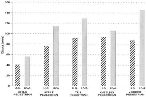
Figure 12. Pedestrian scenes — recognition distances.
Standard U.S. Low Beams
Standard U.S. Low Beams With UVA
Figure 13. Pedestrian crosswalk scene shown with standard U.S.
low beams (above) and standard U.S. low beams with UVA (below).
Static Testing
Visibility Distances
The static testing procedure had subjects indicate how far away they could see the right edge line and the center lane skip lines. The results are shown in Table 1. With the UVA headlights, the edge line was visible 28.9 m (94.71 ft), or 14.46 percent, farther away than with the U.S. headlights. The centerline with the UVA headlights was visible 27.67 m (90.71 ft), or 49.35 percent, farther away. Both of these differences are very significant. The original Clara Barton Parkway study (Mahach, Knoblauch, Simmons, Nitzburg, Arens, and Tignor, 1997) found similar improvements—specifically, a 35.59-m (116.7-ft), or 24.71-percent, increase in edge line visibility and a 28.95-percent increase in centerline visibility.
Table 1. Visibility distances: static testing.
|
Delineation/Headlights |
Mean
(m) |
No. |
Std.
Dev. |
t |
Signif. |
Right Edge Line — U.S.
Right Edge Line — UVA
Skip Lines in Meters — U.S.
Skip Lines in Meters — UVA
|
199.7
228.6
56.1
83.7 |
38
38
38
38
|
46.6
33.2
12.3
16.6 |
-5.456
-14.250
|
0.000
0.000
|
| 1 m = 3.28 ft |
Subjective Ratings
The subjects in the Clara Barton Parkway study were also asked to rate, using a five-point scale, how visible the pavement delineation was with the U.S. and the UVA headlights. The results of these ratings are shown in Table 2. While 60.5 percent of the subjects rated the UVA headlights as excellent, only 7.9 percent said the U.S. headlights were excellent. This compares favorably with the original Clara Barton Parkway study where 75 percent of the subjects rated the UVA headlights as excellent and 8 percent of the subjects rated the U.S. headlights similarly.
Table 2. Subjective ratings: static testing.
|
Headlight Condition |
No. |
Percentage of Subjects Rating Visibility of Roadway Markings as |
|
1
Poor |
2 |
3 |
4 |
5
Excellent |
|
U.S.
UVA |
38
38 |
0
0 |
13.2
5.3 |
57.9
7.9 |
21.1
26.3 |
7.9
60.5 |
Driver Performance Measures - DASCAR
The DASCAR instrumentation in one of the UVA-equipped experimental vehicles allowed several driver performance measures to be monitored. It was hypothesized that improved headlighting/roadway delineation might result in increased vehicle mean speed and reduced speed and lateral placement variances.
The DASCAR collected data every 1/30th of a second. This included data on speed, left-lane lateral placement, right-lane lateral placement, throttle position, hard wheel data from string pot, lateral acceleration, longitudinal acceleration, yaw rate, and braking. For each subject, the number of times the brake was applied, and means and standard deviations for the remaining variables were computed for each of the eight segments for each of the last four laps and across the eight segments for each of the last four laps. The brake number and the means and standard deviations constituted the data set that was used to compare the four different headlights.
The use of parametric statistics for data analysis assumes that variables have normal distributions in the population. Since this could not be assumed for the data, non-parametric statistics for related samples were used. Comparisons between all four headlights were made using the Friedman two-way analysis of variance by rank test. Comparisons between the U.S. and U.S./UV headlights were made using the Wilcoxon signed-rank test. Each of the 8 segments and across all segments were analyzed for headlight differences for 17 variables:
(1) mean and (2) standard deviation of speed
(3) mean and (4) standard deviation of left-lane lateral placement
(5) mean and (6) standard deviation of right-lane lateral placement
(7) mean and (8) standard deviation of throttle position
(9) mean and (10) standard deviation of hand wheel
(11) mean and (12) standard deviation of lateral acceleration
(13) mean and (14) standard deviation of longitudinal acceleration
(15) mean and (16) standard deviation of yaw rate
(17) number of times brake was applied
Significance level was set at p=0.05. Given the large number of statistical tests, it would be expected that 5 percent of these tests would show significant headlight differences by chance. The number of tests with significant differences barely exceeded this level.
Speed
The DASCAR vehicle speed data is shown in Table 3. Although the mean speeds varied 41.81 km/h (25.97 mi/h) for the U.S. headlights to 42.36 km/h (26.31 mi/h) for the UVA headlights, these differences are quite small and not significant. The standard deviations of vehicle speed were also nearly identical—4.72 km/hr (2.97 mi/h) to 4.91 km/h (3.05 mi/h) across the four headlight conditions.
Table 3. DASCAR data: speed.
|
Measure/Headlight Condition |
Mean |
No. |
Std. Dev. |
Friedman Signif. |
Speed — Average (km/h)
Euro
U.S.
Euro/UVA
UVA
Speed — Standard Deviation (km/h)
Euro
U.S.
Euro/UVA
UVA |
42.02
41.81
41.89
42.36
4.78
4.78
4.70
4.91 |
18
18
18
18
18
18
18
18
|
4.83
4.06
5.12
4.94
0.98
0.77
0.89
0.68
|
0.300
0.801
|
| 1 km/h = 0.621 mi/h |
Lateral Placement
The DASCAR lateral placement data is shown in Table 4. The values shown are the distance (in centimeters) from the left side of the vehicle to the roadway centerline. Although a difference in the average lateral placement value was not expected, it has been suggested that better lighting/delineation might help drivers do a better job of tracking within the lane and, therefore, result in reduced lateral placement variance. As shown, the standard deviation values for the four headlight conditions are nearly identical, and not statistically different.
Table 4. DASCAR data: vehicle lateral placement.
|
Measure/Headlight Condition |
Mean |
No. |
Std. Dev. |
Friedman Signif. |
Lateral Placement — Average (km/h)
Euro
U.S.
Euro/UVA
UVA
Lateral Placement — Standard Deviation (km/h)
Euro
U.S.
Euro/UVA
UVA |
88.39
89.85
89.97
90.30
12.35
12.04
12.32
12.36
|
18
18
18
18
18
18
18
18
|
6.20
6.17
5.43
5.38
2.62
2.40
2.61
2.96
|
0.371
0.595
|
| 1 km/h = 0.621 mi/h |
The DASCAR data for brake applications and steering input (amplitude and direction) were also analyzed, but no significant effects were found.
Apparently, the dramatic increases in detection and recognition distances associated with the UVA headlights do not translate to a measurable change in the driver performance measures examined. This was probably because the relatively new delineation in combination with any of the headlights tested was more than adequate to optimize driver speed maintenance and lane tracking.
Subjective Ratings
Part of the experimental procedure involved having the experimental subjects provide a subjective rating of the performance of the various headlights being tested. They were asked to observe the headlights and roadway markings and were asked two questions:
- How do the headlights and roadway markings work compared to those you generally see when driving at night?
- How well did these headlights and roadway markings work for helping you see where to steer the car?
The results of these subjective evaluations are presented in Tables 5 and 6. Table 5 shows the responses to the first question, "How do the headlights compare to what you generally see?" The DASCAR vehicle had four different headlight configurations. The UVA headlights with U.S. low beams were rated as "better than" what they generally see by 76.5 percent of the subjects. The next best headlight condition was the Euro low beams with the UVA headlights. They were rated "better than" by 65.6 percent of the drivers. Interestingly, the Euro low beams (without the UVA headlights) were rated as "better than" by 50.0 percent of the drivers, while the U.S. headlights alone were the most poorly rated, only 32.4 percent of the drivers thought they were better than what they generally see. The Volvo used for the Loops Drive portion of the study had two sets of headlights—regular low beams and the UVA headlights. The differences in subjective ratings are very dramatic. While 73.0 percent of the subjects rated the combined U.S./UVA headlights as "better than," only 43.2 percent rated the U.S. low beams alone as "better than."
Table 5. Subjective ratings:
how headlights compare to what you generally see.
|
Headlight Condition |
No. |
Percentage of Subjects Rating Headlights/Delineation |
|
Not As
Good As |
As Good
As |
Better
Than |
DASCAR
(Subject as Driver)
Euro
U.S.
Euro/UVA
U.S./UVA
Loops Drive
(Subject as Passenger)
U.S.
U.S./UVA
|
32
34
32
34
37
37
|
3.1
8.8
15.6
14.7
10.8
10.8
|
46.9
58.8
18.8
8.8
45.9
16.2
|
50.0
32.4
65.6
76.5
43.2
73.0
|
The subjective ratings in response to the second question—"How do the headlights compare to those used on the previous trial?"—are presented in Table 6. Our major interest is in the comparisons between the regular U.S. headlights and the U.S. headlights supplemented with the UVA headlights. Therefore, the responses have been sorted so that subjective comparisons to regular U.S. low beams are shown. The order of presentation was counterbalanced. On the DASCAR drive, 67.6 percent of the drivers said that the combined U.S./UVA headlights were "better than" the U.S. headlights alone. On the loops drive, on the inner test track, 56.8 percent of the subjects indicated that the U.S./UVA headlights were "better than" the U.S. headlights alone.
Table 6. Subjective ratings:
how UVA headlights compare to U.S. headlights.
| Test Scenario |
No. |
Percentage of Subjects Rating UVA Headlights Relative
to U.S. Headlights |
| Not As Good As |
As Good As |
Better
Than |
DASCAR Drive
(Subject as Driver)
U.S./UVA
Loops Ride
(Subject as Passenger)
U.S./UVA |
34
37 |
23.5
13.5 |
8.8
29.7 |
67.6
56.8 |
Age Effects
It is generally acknowledged that older drivers do not have as good visual acuity, especially at night, as younger drivers. During subject recruiting, every effort was made to recruit older drivers as experimental subjects. This was done so that we could determine if UVA/fluorescent technology would be beneficial to older drivers. Participation involved driving to the remotely located test facility during twilight and taking part in a procedure that typically lasted until 12:00 a.m. to 12:30 a.m. and then driving home. In spite of the generous incentive ($50), finding older drivers was difficult. A total of 10 of the 38 subjects were age 55 or older.
In order to determine if age had a significant impact on detection and recognition distances, a 2x2 analysis of variance with repeated measures on the second factor was performed on dependent variables. The first factor was age (18-54, 55-76) and the second factor was headlight condition (U.S., UVA).
Analyses of variance were performed on all 20 dependent variables. Significant main effects of age were found for the following 10 dependent variables:
- Right curve — detection distance
- Right curve — recognition distance
- Left curve — visibility distance
- No-passing zone — detection distance
- No-passing zone — recognition distance
- Centerline — visibility distance
- Jogger pedestrian — detection distance
- Jogger pedestrian — recognition distance
- Adult pedestrian — detection distance
- Bike — recognition distance
No significant differences were found for the remaining 10 dependent variables.
The results of the analyses of variance for the 10 dependent variables found to have significant main effects for age are shown in Table 7. Right-curve detection distances, for example, with U.S. headlights were 238.4 m (781.5 ft) for younger drivers and 183.0 m (600.0 ft) for the older drivers. The difference is 55.4 m (181.7 ft). With UVA headlights, the distances were 250.8 m (822.8 ft) for younger drivers and 203.3 m (667.0 ft) for older drivers, a difference of 47.5 m (155.8 ft). The F values for age effects and the resulting significance levels for each dependent variable are also shown. For the right-curve detection distance, the F value for age is 8.807 and the significance level is 0.006.
It is not known why there were significant main effects of age for 10 of the 20 dependent variables examined. Significant main effects were found for some measures that showed very large overall effects (e.g., bike: recognition distance) and relatively small overall effects (e.g., right-curve detection distance), so it does not appear that the older drivers performed worse on the harder tasks or did better on the easier tasks.
The significance levels for the differences between the U.S. headlights and the UVA headlights were found to be consistent with the t-test results discussed earlier. Most importantly, analysis for possible interactions between age and headlight condition (U.S./UVA) found no significant difference. Thus, UVA headlights helped younger drivers and older drivers equally. They do not help older drivers more than they help younger drivers. Although it might have been encouraging to find that older drivers, who did not do as well in 10 of the 20 tests, were helped more by the UVA headlights, such was not the case.
Table 7. Age and headlight condition: 2x2 analyses of variance.
| DEPENDENT VARIABLE |
DISTANCE (m) |
| U.S. Headlights |
UVA Headlights |
| Age 18-54 |
Age 55-76 |
Age 18-54 |
Age 55-76 |
|
| Right Curve: Detection Distance |
238.4 |
183.0 |
250.8 |
203.3 |
F (Age)
Significance |
8.807
0.006 |
| Right Curve: Recognition Distance |
214.6 |
167.8 |
243.0 |
198.3 |
F (Age)
Significance |
7.609
0.010 |
| Left Curve: Visibility Distance |
184.4 |
61.0 |
234.3 |
172.8 |
F (Age)
Significance |
5.759
0.024 |
| No-Passing Zone: Detection Distance |
152.5 |
132.2 |
205.6 |
157.6 |
F (Age)
Significance |
4.425
0.044 |
| No-Passing Zone: Recognition Distance |
116.4 |
81.3 |
169.5 |
143.0 |
F (Age)
Significance |
5.976
0.020 |
| Centerline: Visibility Distance |
58.7 |
48.7 |
86.6 |
75.3 |
F (Age)
Significance |
5.026
0.031 |
| Jogger Pedestrian: Detection Distance |
129.3 |
81.3 |
268.5 |
223.7 |
F (Age)
Significance |
12.275
0.002 |
| Jogger Pedestrian: Recognition Distance |
90.8 |
71.2 |
159.8 |
91.5 |
F (Age)
Significance |
6.169
0.020 |
| Adult Pedestrian: Detection Distance |
120.7 |
76.3 |
160.1 |
106.8 |
F (Age)
Significance |
11.930
0.002 |
| Bike: Recognition Distance |
68.6 |
35.6 |
242.7 |
218.6 |
F (Age)
Significance |
4.665
0.040 |
Previous | Table of Contents | Next
|