U.S. Department of Transportation
Federal Highway Administration
1200 New Jersey Avenue, SE
Washington, DC 20590
202-366-4000
Federal Highway Administration Research and Technology
Coordinating, Developing, and Delivering Highway Transportation Innovations
| REPORT |
| This report is an archived publication and may contain dated technical, contact, and link information |
| Publication Number: FHWA-HRT-11-043 Date: December 2012 |
Publication Number: FHWA-HRT-11-043 Date: December 2012 |
PDF files can be viewed with the Acrobat® Reader®
This report describes a methodology for measuring pedestrian and bicyclist exposure based on counts of pedestrian and bicyclist volumes as well as the distances that pedestrians and bicyclists travel on facilities shared with motor vehicles. The distances that pedestrians and bicyclists travel on these facilities represent a measure of their exposure to the risk of having a crash with a motor vehicle. This methodology has the potential to fill a long-standing technical need for a commonly accepted measure of pedestrian and bicyclist exposure, thereby assisting in evaluating the effectiveness of pedestrian/bicyclist safety programs.
This report should be of interest to highway engineers, traffic engineers, highway safety specialists, safety management specialists, pedestrian and bicyclist coordinators, researchers, and others involved in evaluating the effectiveness of safety improvements designed to benefit pedestrians and bicyclists.
Monique R. Evans
Director, Office of Safety
Research and Development
Notice
This document is disseminated under the sponsorship of the U.S. Department of Transportation in the interest of information exchange. The U.S. Government assumes no liability for the use of the information contained in this document.
The U.S. Government does not endorse products or manufacturers. Trademarks or manufacturers’ names appear in this report only because they are considered essential to the objective of the document.
Quality Assurance Statement
The Federal Highway Administration (FHWA) provides high-quality information to serve Government, industry, and the public in a manner that promotes public understanding. Standards and policies are used to ensure and maximize the quality, objectivity, utility, and integrity of its information. FHWA periodically reviews quality issues and adjusts its programs and processes to ensure continuous quality improvement.
Technical Report Documentation Page
1. Report No. FHWA-HRT-11-043 |
2. Government Accession No. |
3. Recipient's Catalog No. |
||||
4. Title and Subtitle A Distance-Based Method to Estimate Annual Pedestrian and Bicyclist Exposure in an Urban Environment |
5. Report Date December 2012 |
|||||
6. Performing Organization Code: |
||||||
7. Author(s) John A. Molino, Jason F. Kennedy, Patches J. Inge, Mary Anne Bertola, Pascal A. Beuse, Nicole L. Fowler, Amanda K. Emo, and Ann Do |
8. Performing Organization Report No. |
|||||
9. Performing Organization Name and Address Science Applications International Corporation (SAIC) 8301 Greensboro Drive, M/S E 12 3 McLean, VA 22102 |
10. Work Unit No. |
|||||
11. Contract or Grant No. DTFH61-08-C-00006 |
||||||
12. Sponsoring Agency Name and Address Office of Safety Research and Development Federal Highway Administration 6300 Georgetown Pike McLean, VA 22101-2296 |
13. Type of Report and Period Covered Final Report, January 2006-June 2011 |
|||||
14. Sponsoring Agency Code HRDS-30 |
||||||
15. Supplementary Notes The Contracting Officer's Technical Representative (COTR) was C.Y. David Yang (HRDS-30). |
||||||
16. Abstract Currently, there is no commonly accepted or adopted measure of pedestrian and bicyclist exposure. This report presents a methodology for measuring a region's pedestrian and bicyclist exposure, which is defined as 100 million pedestrian/bicyclist mi (161 million pedestrian/bicyclist km) of roadway (or other motor vehicle shared facility) traveled. A method for implementing the exposure measure is described for various shared facility types that are characteristic to the urban environment of Washington, DC. These facilities include three types of intersections (signalized, stop-controlled (all-way), and partially stop-controlled) as well as midblock road segments, driveways, alleys, parking lots, parking garages, school areas, and areas with playing/dashing/ working in the roadway. A pilot study demonstrated the feasibility of the method at seven sites in Washington, DC, in 2006. In 2007, the methodology was implemented on a larger scale to estimate the annual pedestrian and bicyclist exposure in Washington, DC, which was 0.80 hundred million mi (1.29 hundred million km) for pedestrian exposure and 0.37 hundred million mi (0.59 hundred million km) for bicyclist exposure. As a result of simplifications in the present data aggregation technique, these particular exposure values are overestimated. However, procedural changes are suggested to correct this issue. Within the constraints of this study, both the feasibility and scalability of the methodology were successfully demonstrated for a relatively large urban environment. The results indicate that the methodology has the potential to be used to collect exposure data that are not currently readily available to the pedestrian and bicycle safety community. Although further refinement and validation are still needed, the methodology provides a possible initial foundation to develop a national unit of exposure for pedestrians and bicyclists. |
||||||
17. Key Words Pedestrian exposure, Bicyclist exposure, Exposure to risk, Roadway safety, Shared transportation facilities, Pedestrian and bicycle safety |
18. Distribution Statement No restrictions. This document is available through the National Technical Information Service, Springfield, VA 22161. |
|||||
19. Security Classif. (of this report) Unclassified |
20. Security Classif. (of this page) Unclassified |
21. No. of Pages 83 |
22. Price N/A |
|||
| Form DOT F 1700.7 | Reproduction of completed page authorized |
SI (Modern Metric) Conversion Factors
Chapter 4. Discussion and Conclusions
Appendix A. PHASE II DATA COLLECTION FORMS
Appendix B. SIGNALIZED INTERSECTION CALCULATION EXAMPLE
Pedestrian fatalities resulting from traffic crashes in the United States have decreased over the past decade from 5,228 in 1998 to 4,378 in 2008. Similarly, the number of bicyclist fatalities has decreased by 5.7 percent from 760 in 1998 to 716 in 2008.(1) While this decrease could be a result of several factors, it is difficult to identify the specific ones without knowing the exposure of pedestrians and bicyclists. For example, the reduction in fatalities could be caused by improved safety countermeasures, but it could also be due to fewer people walking and bicycling.
With regard to pedestrian/bicyclist safety, exposure is defined as pedestrian/bicyclist proximity to potentially harmful situations involving motor vehicles (i.e., crossing an intersection). Exposure is related to the opportunity to have a crash and represents a precondition that must be present in order to have a crash. Pedestrian/bicyclist risk is defined as the probability that a pedestrian/bicyclist-motor vehicle crash will occur based on the exposure. This report describes a methodology to measure a region's pedestrian/bicyclist exposure.
The Federal Highway Administration (FHWA) and National Highway Traffic Safety Administration (NHTSA) are the primary agencies responsible for the data that form the basis of the annual motor vehicle fatality rate in the United States (fatalities per 100 million mi (161 million km) traveled). Crash data (numerator) are available from NHTSA's Fatality Analysis Reporting System for fatalities and from the National Automotive Sampling System General Estimates System for other types of crashes.(2,3) Exposure data (denominator), in terms of 100 million vehicle mi (161 million km) traveled (VMT), are available through FHWA's Highway Performance Monitoring System.(4)
Currently, pedestrians and bicyclists are not accounted for in the denominator of this ratio even though pedestrian/bicyclist fatalities are included in the numerator. However, to adequately conduct pedestrian and bicyclist crash analyses, it is essential to determine their exposure. In 2000, NHTSA and FHWA conducted a series of pedestrian and bicycle strategic planning workshops. Out of a total of 57 pedestrian and 57 bicycle research needs, the lack of adequate pedestrian and bicyclist exposure data ranked in the top category among the 4 highest priority research needs for both pedestrian and bicyclist research.(5)
This report has two major goals: (1) to describe a methodology for measuring pedestrian/ bicyclist exposure and (2) to demonstrate the application of this methodology by calculating the annual pedestrian and bicyclist exposure for a large urban environment in terms of 100 million pedestrian/bicyclist mi (161 million pedestrian/bicyclist km) of roadway or motor vehicle shared facility traveled.
A variety of pedestrian/bicyclist exposure measures has been developed and applied in the past. These measures focus on population pedestrian/vehicle volumes, time, and distance. The following sections describe a small but fairly representative sample of studies that investigated each of these metrics.
Population measures have been proposed as an estimator for motor vehicle and pedestrian/ bicyclist exposure to risk. The supposition is that crashes between motor vehicles or crashes between pedestrians/bicyclists and motor vehicles are more likely to occur when there are more residents, drivers, motor vehicles, pedestrians, bicyclists, or bicycles in a given area. It might be expected that fewer crashes or fatalities would occur in areas with a low population density of people, motor vehicles, and/or bicycles. Over the past several years, NHTSA has annually reported the number of motor vehicle fatalities and fatality rates based on three population types in the United States in their Traffic Safety Facts technical briefs.(1) In 2007, motor vehicle crashes resulted in 13.68 people killed per 100,000 residents, 20.05 people killed per 100,000 licensed drivers, and 16.13 people killed per 100,000 registered motor vehicles.(1) However, such population-based methods have limited use when examining pedestrian/bicyclist crashes since these methods do not consider the opportunity of exposure to motor vehicles, especially at a specific type of location (e.g., a roadway). Traditional population metrics have not been sensitive to the amount of time or distance that a pedestrian or bicyclist is exposed to motor vehicle traffic. Additionally, traditional population metrics have not accounted for external changes in behavior patterns, such as changes in walking or bicycling behavior for health or environmental reasons with a constant population of residents, bicyclists, and/or bicycles.
In a study conducted by Rodgers, exposure based on bicyclist population was estimated from data collected in a survey conducted by the Consumer Product Safety Commission (CPSC).(6) CPSC conducted a random-digit-dial telephone survey to gather information on bicycle use in the United States. One person per household was contacted via a stratified random selection process and was interviewed. CPSC collected information on the number of bicyclists and bicycles in use, the demographic characteristics of the rider households, rider characteristics and use patterns, helmet use, and the types of bicycles used. From the 1,254 completed survey interviews, CPCS estimated that 66.9 million bicycle riders lived in about 27.1 million households in 1991. The 27.1 million households with bicycle riders represented an estimated 28.8 percent of the total U.S households (94 million) in 1991. Based on these statistics, it was estimated that there were about 12 crash-related deaths per 1 million bicyclists that year. Presumably, such crash rate statistics could be tracked for different years to evaluate trends in overall bicyclist safety. However, such a population-based bicyclist exposure metric suffers from the deficiencies mentioned earlier-insensitivity to location factors (riding on a road versus on a trail) and rider behavior changes due to external circumstances (riding to protect the environment from pollution) and not related to changes in bicyclist or bicycle population density. Such a population-based metric also runs counter to the notion of "safety in numbers," as proposed by Jacobsen.(7) Jacobsen hypothesized that the more dense the population of pedestrians or bicyclists, the lower the probability of a crash.
One measure of pedestrian exposure that has been investigated in the past is the number of pedestrians observed in the roadway. Ivan et al. conducted a pedestrian exposure study in rural Connecticut.(8) The authors counted the number of pedestrians crossing streets and the number walking along the highway. Weekend and weekday manual counts were conducted at 32 sites, and observations took place from 8 a.m. to 5:30 p.m. They also investigated the relationship between the weekly pedestrian exposure in rural areas of Connecticut and factors such as population density, the existence of a sidewalk system, the number of traffic lanes, area type, traffic signal type, and median household income. Linear statistical modeling methods were used to examine how a response variable may depend on one or more explanatory variable. It was found that exposure did not vary significantly with population density in the walking area. Traffic signal type and median household income were also not significant factors. Area type (e.g., downtown, commercial, residential, etc.) was significant for pedestrian volume, as were the number of traffic lanes and the existence of a sidewalk system. This study was limited to pedestrian crossing volumes in rural areas of Connecticut. As a result, exposure may not be the same for other regions. The authors suggested that pedestrian safety analyses based on population density may distort risk values. This study employed only the number of pedestrians observed in the roadway to develop an exposure metric. It did not include the number of motor vehicles observed and reflected only changes in walking behaviors, and not driving behaviors. This measure is similar in concept to the one tested in the present study, but it does not incorporate a distance metric to differentiate between short and long distances of pedestrian/ bicyclist exposure to motor vehicle traffic.
A study by Silcock et al. also used the number of pedestrians crossing the street as the exposure measure.(9) Nine busy urban sites in the United Kingdom were investigated. Video was recorded, and the number of crossing movements and the interactions between pedestrians and motor vehicles was coded. Automatic image processing was used to count the number of motor vehicles and pedestrians. The study reported an accuracy of more than 90 percent for motor vehicle counts and more than 85 percent for pedestrian counts. In total, 32,000 pedestrian crossing events were recorded. The study recommends the use of a pedestrian/motor vehicle conflict measure by creating a pyramid of crossing events ranging from nonrated crossings to encounters, conflicts, and collisions. In this formulation, conflicts are defined in terms of evasive maneuvers taken by either the pedestrian or the driver, and motor vehicle counts and maneuvers are an important part of the metric.
Zegeer et al. also counted the number of pedestrians crossing the roadway as a measure of exposure.(10) The study employed 15-min counting periods for 1 h of observations at each site. Additionally, an expansion factor was developed to fill in the data for those periods that were not observed. The authors estimated pedestrian average daily traffic for 1,000 sites with marked pedestrian crosswalks and for 1,000 sites with unmarked pedestrian crosswalks, all without traffic signals or stop signs.
In a study conducted by Cameron and Milne, an exposure measure was proposed using pedestrian and motor vehicles volumes.(11) The exposure metric consisted of multiplying pedestrian volumes by motor vehicle volumes (P × V), which was used to investigate the relationship between pedestrian/motor vehicle conflicts and crashes. Davis et al. also employed P × V as an exposure measure.(12) Empirical data were collected manually in two cities, and historical data were obtained from local transportation agencies. The historical data pertained to the number of crashes over a 3-year period. Manual counts were conducted over 9 months during a 6-h (7-9 a.m., 11 a.m.-1 p.m., and 4-6 p.m.) weekday data collection period. Intersections were counted for 5-min periods, and each approach or crosswalk was sampled at least three times during each data collection hour. In total, 48 intersections were included in the study, with 24 in each city. The study found that using the P × V measure can distort estimates of crashes based on conflicts. For example, if 20 cars and 20 pedestrians are at a given location, there would be 400 potential conflicts. There would also be 400 potential conflicts if 2 pedestrians and 200 motor vehicles were at a given location. However, depending on the circumstances at each location, the crash rates could be different.
Tobey et al. also used the P × V exposure measure.(13) In total, 1,357 sites were measured in several cities where researchers counted 612,395 motor vehicles and 60,906 pedestrians. Pedestrian and motor vehicle data were manually collected during 15-min segments at each site. Motor vehicle and pedestrian exposure data were defined in terms of volume counts and action data. The action data described motor vehicle and pedestrian behaviors. Pedestrian action data included the number of pedestrians crossing within a crosswalk, crossing within 50 ft (15.2 m) of a crosswalk, crossing midblock, and diagonally crossing the intersection. In total, 12,528 h of pedestrian and motor vehicle activity were observed and recorded. Crash data were combined with the estimated P × V exposure data to compute relative "hazardousness" scores for various roadways and intersections as well as pedestrian and motor vehicle characteristics.
The P × V exposure measure enabled the research team to identify pedestrian trip characteristics, develop pedestrian exposure measures, and determine the relative hazard associated with various pedestrian characteristics and behaviors. Primary sampling units were defined to facilitate extrapolation to aggregated measures. Weighting procedures were used to calculate hourly pedestrian volumes and to project those hourly volumes to an entire week of pedestrian activity. The sample locations were weighted to represent an entire city and were further weighted to represent the entire country. The present study used a similar overall approach but with different weighting techniques to generalize from 15-min counts of pedestrians and bicyclists to the estimated annual exposure for an entire city.
The publications by Cameron and Milne, Davis et al., and Tobey et al., all employed the P × V metric for pedestrian exposure to capture the concept of potential pedestrian and motor vehicle conflicts.(11-13) One potential problem with this method is that the pedestrian and motor vehicle volumes must refer to a relatively brief time separation and a relatively short distance separation in order for them to reflect the potential for true conflict. If the motor vehicle passes at a different time than when the pedestrian crosses the street or if the motor vehicle passes far away from where the pedestrian is in the crossing path, the possibility of a crash is diminished.
The amount of time that a pedestrian or bicyclist engages in certain activities may be taken as a measure of exposure. Keall conducted an exposure study using the New Zealand travel survey (1989-1990) in which respondents were asked to record information regarding their walking behavior.(14) The survey was collected from a random sample of New Zealand residents who were over the age of 5. In total, 8,719 people completed the survey and were given diaries to record basic details of trips made during two specified days of the survey period. Personal interviews were also conducted to collect more information regarding travel. This study examined time spent walking and the number of roads crossed to determine exposure. Some trips less than 328 ft (100 m) long were not recorded in this survey depending on the nature of the trip. An adult was interviewed for participants ages 5-11 to determine exposure. It is worth noting that past studies have shown that adults tend to underestimate children's exposure. Also, it may have been difficult for people to estimate the amount of time that they spent walking and the number of roads that they crossed.
In a study conducted by Chu, exposure was estimated using self-reported data on trip duration from the 2001 National Household Travel Survey (NHTS).(15) The 2001 NHTS was used to collect data from one-way trips taken during a designated travel day by a national random sample of 26,028 households. The data included travel by people of all ages. Travel days were assigned to all days of the week and all seasons from April 2001 to April 2002. One limitation with this study was that the information was derived from "perceived travel time" for walking. Walking time may have been inaccurately reported due to forgetfulness or people purposely not reporting. Another problem with the survey was that the reported walking may have been completed along shared use paths, in the woods for exercise purposes, or in situations that may not represent exposure to motor vehicle traffic (e.g., walking on sidewalks, up stairs, and to platforms in train stations). Walking reported on facilities that pedestrians and motor vehicles do not share can result in overestimating the exposure.
Bly et al. conducted a study to observe the differences in exposure and accident rates of children ages 5-15 in Great Britain.(16) The exposure measures used for this study were the amount of time children spent walking in different road environments and the number of times they crossed a road in each environment. A home interview was conducted with participants to determine their out-of-home activity for the previous day. Following the home interview, the interviewer re-walked the route to collect more information about the environment. This technique was used to conduct a comparative study on the relative exposure of children in Great Britain, France, and the Netherlands. Time spent walking near roads was found to be similar in all three countries, but Great Britain had less road crossing activity. Children in the Netherlands spent substantially more time bicycling than in the other two countries. In Great Britain, the total time exposure was greater in cities than in towns or rural areas. In France, this difference was less pronounced. In general, the differences in total exposure could not explain the higher overall crash rates for children in Great Britain.
Both of the above studies employed the amount of time walking as one measure of exposure. This measure has the advantage of capturing time differences between pedestrians who walk more and those who walk less. However, the measure is not sensitive to where people walk. As a result, it includes time walking on sidewalks, trails, and other facilities not shared with motor vehicles. The time spent walking in these facilities represents an overestimate of exposure because the likelihood of a crash between a pedestrian and a motor vehicle is extremely small at these locations. If the measure had specified time spent walking in locations where pedestrians and motor vehicles share the same facility, the time metric would have represented a variant of the metric in the current investigation, the difference being time walking in the facility would have replaced distance walking in the facility. For a constant walking speed, the distinction between time walked and distance walked is minimal. The distance metric was preferred in this study because highway engineers tend to work with distances more than with time, and VMT for motor vehicles is based on distance.
Distance traveled is considered a measure of exposure. In a study conducted by the Bureau of Transportation Statistics in London, England, researchers used walking distance traveled as the exposure metric.(17) The main source of information for this study was the National Travel Survey. This survey provides information about personal travel and other factors that may influence it. It has been conducted annually in Great Britain since 1988. Based on the data from this survey, an estimate of distances traveled was compared to casualty rates to compute risk. The National Travel Survey tends to underestimate walking distances because certain types of activities are not included in the survey (e.g., short trips (less than 150 ft (45.7 m)), children playing in the streets, walking required for work (e.g., postmen), etc). Consequently, risk estimates for pedestrians are likely to be overestimates.
Kaplan conducted a study of adult bicyclists to estimate bicyclist miles traveled.(18) A survey was conducted to obtain demographic and bicyclist description information, trip characteristics, and accident experience from 3,270 adult bicyclists for 1 calendar year. The bicyclist miles traveled were estimated from the respondents' odometer readings or other estimation techniques. Over one-third of the respondents used an odometer, and the others reported consistent distances traveled for equivalent circumstances. Respondents reported that they traveled by bicycle for an average of 2,332 mi (3,752 km) over an average period of 8.9 months. Using the bicycle miles as an exposure measure, Kaplan found that age, gender, and years of rider experience influenced the crash rate.
Both of the above studies used distance traveled as a measure of exposure, similar to the present study. The difference is that these previous investigations used total distance traveled, not just distance traveled on facilities shared with motor vehicles such as roadways, driveways, parking lots, etc. These earlier investigations included distances traveled on sidewalks, trails, and other segregated facilities. Consequently, exposure was overestimated, and risk was underestimated. If a more restrictive definition to include only facilities shared by pedestrian/bicyclists and motor vehicles had been invoked, the above studies would have employed a metric identical to the one tested in the present study. However, those studies used social surveys, which generally do not have the accuracy of direct observational counts of pedestrian and bicyclist activities. Social surveys are primarily based on a person's memory of a certain behavior rather than direct observation of that behavior.
The described pedestrian and bicyclist exposure methodology differs from the four metrics described in the literature review. The methodology, described in detail in chapter 2 of this report, uses motor vehicle exposure analog as a point of departure. While 100 million VMT (161 million km) is used for motor vehicle exposure, pedestrian/bicyclist exposure is defined as 100 million pedestrian/bicyclist mi (161 million pedestrian/bicyclist km) of roadway traveled.(4) Specifically, it is defined as 100 million pedestrian/bicyclist mi (161 million pedestrian/bicyclist km) of shared facilities traveled including parking lots, driveways, alleys, parking garages, and other facilities where pedestrians and bicyclists share the same space with motor vehicles. This exposure measure is closest to the pedestrian volume crossing the street and walking along the highway measure that has previously been explored because both concentrate on pedestrians walking only on the roadway and not on sidewalks, trails, and other places where motor vehicles are not allowed.(8) In addition to including a bicyclist component, the measure includes distance traveled to incorporate a spatial component to individual exposure to a potentially hazardous environment.
While the overall amount of pedestrian and bicyclist travel, regardless of location, is important for understanding the level of outdoor activity or mobility of a population, this study focused on the amount of walking/bicycling while at risk of being involved in a motor vehicle crash. The pedestrian crash rate is dependent on having a quantity of exposure in the denominator that corresponds with the numerator. Pedestrian and bicyclist travel on nonmotorized facilities, such as shared use paths, was not included because there is a negligible risk of being involved in a motor vehicle crash for that type of travel. Although some types of motorized recreational motor vehicles may be allowed under certain circumstances, the number of pedestrian/bicyclist crashes with such motor vehicles is likely to be small. While the probability of a pedestrian crash with a bicycle is likely to be much higher on such shared use paths, the focus of this study was on pedestrian/bicyclist crashes with motor vehicles. If a new trail, sidewalk, or sheltered facility is being installed, presumably any walking or bicycling on the newly constructed nonmotorized facilities would lower the exposure estimates for nearby facilities shared by pedestrians/ bicyclists and motor vehicles. As a result, the influence of safety countermeasures designed to separate pedestrians and bicyclists from motor vehicle traffic would be reflected in the measure. Additionally, the pedestrian/bicyclist volume estimates derived from the described methodology could be used in applications such as pedestrian/bicyclist crash prediction models and before/ after comparisons. The pedestrian/bicyclist distance estimates derived from the methodology could also be used to identify facilities with long exposure distances for safety improvements (curb extensions, pedestrian bridges, etc) and for studies involving geometric design changes to exposure distance (e.g., roadway widening).
One prominent theme in previous research has been the computation of the product of P × V as a measure of exposure. This approach has the advantage of taking into account the number of potential conflict opportunities between pedestrians and motor vehicles. However, it has the disadvantage of being dependent on changes in motor vehicle behaviors or volumes. The exposure measure in this study is orthogonal to motor vehicle behaviors and is only sensitive to changes in pedestrian and bicyclist behavior patterns. Such independence is considered important so that the metric can adequately reflect changes in walking and bicycling patterns of populations independently of whether the same populations drive more or less over the same time period. In this sense, the metric is similar to the VMT measure used for estimating exposure. The metric is designed to reflect overall patterns in the amount that people walk and bike on roadways and other shared facilities in general. A similar argument is true for the severity of potential crashes. It is desirable to have the exposure metric orthogonal to the crash metric. The exposure measure should be dependent only on walking and biking behaviors and not confounded with the nature of the crashes, which is derived from the crash measure. The exposure metric should directly reflect how much people walk or bike in areas shared with motor vehicles so that it will be sensitive to changes in people's walking and biking patterns.
FHWA researchers collected data using the described methodology in fall 2006 in Washington, DC. Testing indicated that the measure was viable as a possible pedestrian and bicyclist exposure methodology. However, these tests only employed one measurement site for each of seven unique types of pedestrian and bicyclist facilities. The present study measures multiple sites for each type of facility and combines the data from all sites into an overall estimate of pedestrian and bicyclist exposure for Washington, DC, for the 2007calendar year. These estimates of annual exposure for a moderately large American city are regarded as the first step to demonstrate the potential scalability of the methodology for consideration at a national level. If this metric works for one city, it should work for others. There are potential issues with the amount of resources and effort which might be required to collect and aggregate adequate data for all of the different types of pedestrian and bicyclist exposure facilities. However, this load could be potentially shared among a number of cities, with one city concentrating on a given facility type and sharing the information obtained with the other cities to obtain or expand to a national estimate. A summary report was published in 2009 concerning these estimates and the methodology for their derivation.(19)
Pedestrian and bicyclist counts were conducted, and travel distances were measured in Washington, DC, during fall 2006 (phase I) and summer/early fall 2007 (phase II). This time period generally represents the peak time for tourists in the city. The data collection procedure was completely passive, using personnel who observed pedestrian and bicyclist movements while standing on the sidewalk or sitting in a parked motor vehicle. These observers counted the number of pedestrians and bicyclists who traveled in the street or on other motor vehicle shared facilities during 15-min intervals. There was no interference with the flow of pedestrian, bicycle, or motorized traffic, and no personal contact or interviews were conducted.
The observers also estimated the length of crosswalks, roadways, driveways, and parking lots in most cases using previous knowledge of lane widths, car lengths, and other indirect means. At times, more precise measurements were made with tape measures, distance wheels, or remote distance-measuring equipment as a validation check for lane width estimates. For safety reasons, the observers always worked in pairs, and no direct observations were made from 10 p.m. to 6 a.m. All nighttime measurements were made using a sample of the District Department of Transportation's (DDOT) traffic cameras, which were accessed via the Internet.(20)
This study was conducted with significant constraints in terms of time and resources. As a result, simplifications were made in the temporal and spatial sampling and aggregation techniques to generalize the data. As will be explained later in this report, a number of these simplifications likely resulted in an overestimation of annual pedestrian and bicyclist exposure. This overestimation was alluded to in the earlier summary report.(19) This report offers some suggestions to reduce overestimation. The main focus of the study was to develop a methodology for measuring pedestrian/bicyclist miles traveled on facilities shared with motor vehicles. These exposure estimates offered are only used as an example of how the technique might be implemented. Such estimates were never intended as input for engineering or policy decisions and should not be used for such purposes.
This chapter describes the methodology used for the collection, reduction, and analysis of the pedestrian and bicyclist counts and corresponding distances traveled on a facility shared with motor vehicles in an urban environment. It is assumed that modifications are necessary in suburban or rural situations. However, the general techniques described in this chapter are likely to form the basis for most of the variations needed to handle a wide range of situations. The techniques and procedures used were similar in both phases of the study; however, some differences exist and are described in separate subsections in this chapter.
Two trained observers conducted the onsite field data collection. A third trained observer monitored a small portion of the data collection sites using traffic cameras via the Internet. The data collectors used materials and equipment most State and local agencies or organizations would likely have access to with the exception of the agency-installed traffic cameras. Mechanical counters, in conjunction with clipboards and preprinted data collection forms, were employed to passively observe and record pedestrian and bicyclist volumes, distances, and other data (see appendix A for examples of data collection forms). The three-button counters were typically attached to the top of the clipboard with the data collection forms visible below the counters (see figure 1).
Figure 1. Photo. Mechanical counter, clipboard, and data collection form.
The data collectors used a variety of instruments to measure (and estimate) roadway distances. These instruments included a motor vehicle-based distance-measuring instrument (DMI), a hand-wheel, measuring tape, hand-held laser DMI, and distance-measuring tools associated with geographic information system (GIS) and satellite imagery software. In the case of play/work in the roadway situations, the observers used a stopwatch to record durations spent in a shared facility by pedestrians who were chatting, bicyclists who were stopped, children who were playing, people who were repairing automobiles, etc. These people lingered in the shared facility for a considerable amount of time and did not simply transit through the measurement area from one end to the other.
The same materials and equipment used in phase I were also used in phase II. However, in phase II, additional data sources were required to estimate the total population of each type of facility in Washington, DC. DDOT provided a list of the locations of all signalized intersections in the city.(21) Satellite imaging software was used to measure and confirm the width of roads and to provide estimated counts of all stop-controlled intersections, partially stop-controlled intersections, parking lots, and driveways throughout the city. GIS software was used to estimate the total number of alleys, and the Yellow Pages was used to estimate the total number of parking garages.(22,23) An inventory of public schools was obtained from the Washington, DC, Public School System.(24) A standard statistical software package was used to perform linear statistical modeling on the signalized intersection data.(25)
Phase I was a pilot study intended to provide preliminary feedback to the researchers about the basic feasibility of conducting the more comprehensive and detailed data collection endeavor proposed for phase II. Therefore, only seven sites were selected (signalized intersection, stop-controlled intersection, midblock location with no crosswalk, driveway/alley, parking lot/parking garage, play/work in roadway, and midblock location with crosswalk), one site for each type of shared use facility of interest. Six of these sites were the same type as those measured in phase II, and one site (midblock location with crosswalk) was of interest to DDOT. It was not measured in phase II because few of them exist in Washington, DC. The seven sites were selected based on feedback from DDOT and other stakeholders, as well as the researchers' general knowledge of the city. Table 1 shows the seven sites in phase I.
Table 1. Phase I locations.
Facility Type |
Site Location |
|---|---|
Signalized intersection* |
Wisconsin Avenue and M Street NW |
Stop-controlled (all-way) intersection |
S Street and 19th Street NW |
Midblock location with no crosswalk |
I Street between 18th Street and 19th Street NW |
Driveway/alley |
Macomb Street between Connecticut Avenue and Ross Place NW |
Parking lot/parking garage |
The Home Depot® parking lot at 901 Rhode Island Avenue NE |
Play/work in roadway |
100 Block Bryant Street NE |
Midblock location with crosswalk |
Howard Road SE in front of Anacostia Metro Station |
* Indicates data were sampled over 24 h at this facility type.
Some of the sites were selected because of their significant pedestrian/bicyclist volumes so that adequate data could be collected to test the techniques and methods within the limited resources of the pilot study. When possible, geographic diversity was also considered for site selection by ensuring that the sites were located in different parts of the city. All sites were observed multiple times, and one site (the signalized intersection) was sampled over 24 h, with various time periods sampled on different days.
One goal of the study was to collect data at approximately 100 sites spread out over 8 facility types. This number was dictated by the time and resources available to conduct the study. In total, 122 locations were sampled, resulting in 364 unique 15-min counts. Each data collection period typically involved two different locations in close proximity, with the exception being parking lots and parking garages. Once the first site was chosen (using the sampling variables described below), the second site in that time period was chosen based on proximity to the first. The two sites measured in a single time period were usually a similar facility type, although this was not required. In addition, locations that had planned construction/work zones were excluded from the sample. Even though such construction sites could in some cases increase exposure due to closed sidewalks, in other instances, roadway work zones could reduce exposure by obstructing pedestrian and bicyclist crossings. In either case, such locations represented a small portion of all possible locations in the city and should not be considered to be either a representative or statistically adequate sample. Future implementations would need to improve the sample size and composition.
Instead of having an equal number of sites per facility type, each facility type was assigned a number of sites based on assumed activity levels. For example, because intersections have considerable pedestrian and bicyclist activity, they were sampled more than some other facility types. While this tendency to sample locations with higher pedestrian and bicyclist activity led to more accurate estimates of counts for single locations, it also led to overestimation in the aggregation process across locations. Future implementation of the procedure should sample facility types in closer proportion to the total number of facilities of that type present.
Observations of pedestrian/bicyclist volumes and distances were sampled for the following eight facility types:
Six sampling variables were used in the site selection process (see table 2). The first three sampling variables represent the temporal distribution of measurement samples across different hours of the day, time periods, and days of the week. The last three variables represent the spatial distribution of measurement samples across various geographical regions of Washington, DC, divided by land use, zoning, and political district (ward). Column 2 shows the number of categories per variable. The number of categories for hour of day is 24, and the number of categories for day of week is 7. The day was also divided into seven time periods: morning, midmorning, noon, afternoon, early evening, late evening, and night. Land use type was divided into seven designations used by Washington, DC: low density residential, medium density residential, high density residential, public/open space, Federal/local/mixed use/public institutional, industrial, and commercial. Zoning type was also divided into seven similar designations. Ward was divided into eight geographical areas according to population, so each ward had about the same number of residents. Column 3 shows the mean for the number of observation locations per category out of the 122 total locations sampled. Columns 4 and 5 show the minimum and maximum number of observation locations per category, respectively.
Table 2. Sampling variables and their spatial characteristics.
| SamplingVariable | Number of Categories Per Variable | Mean Number of Locations Per Category | Minimum Number of Locations Per Category | Maximum Number of Locations Per Category |
|---|---|---|---|---|
Hour of day |
24 |
12.3 |
1 |
27 |
Time period |
7 |
16.7 |
13 |
20 |
Day of week |
7 |
17.0 |
9 |
25 |
Land use type |
7 |
17.4 |
1 |
44 |
Ward (district) |
8 |
15.3 |
13 |
19 |
Zoning type |
7 |
17.4 |
1 |
44 |
As shown in table 2, time period, day of week, and ward all had relatively uniform sampling distributions along the spatial dimension (i.e., the number of different observation locations per category). For these three variables, the mean number of locations per category was between 15 and 17, and the range from the minimum to the maximum was within about 30-50 percent of the mean and evenly distributed above and below the mean. Hour of day, land use type, and zoning type had less uniform distributions with a much wider range. Some categories had only a single observation location. Hour of day had substantially less locations sampled at night because there were fewer pedestrians present at night, and the security of the observers was an issue. Land use type and zoning type also had substantially fewer locations in industrial and manufacturing areas because Washington, DC, is not primarily an industrial city.
The primary spatial sampling unit was arranged by ward because they were a primary classification scheme for demographic data. Where possible, a roughly equal number of facility types was sampled from each ward. Because the wards were roughly equated to population, densely populated downtown areas were much smaller in geographical size and contained fewer examples of certain prominent facility types (e.g., proportionately less intersections and less stop-controlled intersections). Furthermore, whatever few stop-controlled intersections might be present in such downtown areas would likely have a higher than average pedestrian and bicyclist volume. By contrast, the higher number of less busy stop-controlled intersections in more suburban-type residential areas would be relatively undersampled. In future studies, the number of facilities sampled per ward should be weighted by the relative number of those facilities present. If implemented for all facility types, such an adjustment would not only preserve the spatial dispersion across population areas, but also reduce the tendency to overestimate the final measure of annual pedestrian and bicyclist exposure.
Using the sampling variables listed above, researchers developed two stratified spatial sampling procedures: one variation for signalized intersections and school crossing areas and another variation for the other six facility types to obtain an adequate spatial distribution of measurements across different areas of the city. Each of the 122 locations, with the exception of 3, was observed 1-4 times, usually during the same day. Additionally, 3 locations were selected for observation 18-38 times over several days of the week to investigate temporal variation in more detail. The three locations selected for more detailed temporal sampling were all signalized intersections representing two different land use areas (one residential and two commercial) and three different wards.
Signalized intersection locations were selected from a list maintained by DDOT of the 1,581 signalized intersections in Washington, DC.(21) The selection process consisted of a researcher pointing at random to one of the signalized intersections on the DDOT list, identifying the category for each of the three spatial sampling variables (see table 2) for that location, and checking those categories against the data collection schedule to decide whether such a location needed to be sampled or not. The three temporal variables were considered only secondarily. This process was repeated until the required number of signalized intersections was reached. While not all combinations of all categories across the six sampling variables were represented in the final sample of sites, an attempt was made to make the sample as representative as possible across the sampling variables and their categories.
The site selection process for the remaining six facility types was slightly different. Except for schools, no list similar to that for the signalized intersections existed for the remaining facility types. The locations were chosen using land use, zoning, and ward maps of Washington, DC. A researcher pointed at random to an area on one of the maps without purposely looking for any particular location within the city. Once a location was identified, the three primary spatial sampling variables (land use, zoning, and ward) and the three temporal sampling variables (hour, time period, and day) were checked against the data collection schedule to decide whether or not such a location needed to be sampled. This process was repeated until the required number of sites was reached for each facility type.
For the calculation of bicyclist distances traveled, it was necessary to estimate the average block length for the city. A single block length was assumed for all blocks sampled. Although there are exceptions, Washington, DC, has consistent block lengths. The city has a diagonally crisscrossing system of avenues, but this system can be regarded as an overlay and does not perturb the basic underlying square block grid. In total, 83 block segment lengths were sampled that were proportionally distributed across wards for the entire city. The average block length was about 500 ft (152 m) with a standard error of ±20 ft (±6.1 m), which was employed to characterize all blocks. In future studies, if a city has regular blocks, this single estimate technique may still be applicable. However, if a city has irregular blocks or if resources permit the measurement of each individual block length, it would be desirable to measure the adjacent legs of each block sampled.
In this study, the procedures used to select locations for measurement were not entirely random. While it would have been relatively easy to use a pseudo-random number generator to select from the stratified lists of signalized intersections, such a procedure was not possible for the other facility types. Larger sample sizes will be required for future elaboration of the methodology. In that case, the locations would need to be sampled by a more rigorous method, perhaps by applying a numbered grid to each of the maps and employing a pseudo-random number generator to select locations from the grid.
General information was collected at all sites for each data collection visit. Observers recorded the address, date, shift time, day of the week, weather, and observers' names on a form. They then drew a sketch of the data collection location. For each of the 15-min counts, pedestrian and bicyclist volumes were recorded on mechanical counters. Crossing distances for all roadways, intersection legs, driveways, etc., were also recorded. The three-button mechanical counters (see figure 1) were used to count pedestrians in the crosswalk (one foot in the crosswalk for at least half of the crossing distance), pedestrians not in the crosswalk (jaywalkers), and bicyclists traversing the data collection zone. An average diagonal crossing distance was applied to jaywalking counts.
Facility-specific data collection procedures are included in the following sections.
In this study, intersections were categorized by level of traffic control. The three levels were signalized, stop-controlled (all-way), and partially stop-controlled (one- or two-way). Typical examples of these three types of intersections are shown in figure 2 through figure 4.
Figure 2. Photo. Example of a signalized intersection.
Figure 3. Photo. Example of a stop-controlled (all-way) intersection.
Figure 4. Photo. Example of a partially stop-controlled (one- or two-way) intersection.
For signalized and stop-controlled (all-way) intersections, one observer stood on the sidewalk at one corner of the intersection, and the second observer stood on the sidewalk at the diagonally opposite corner. Both observers faced the center of the intersection and were responsible for both legs of the intersection (road and crosswalk) to their immediate left, creating two separate zones split diagonally down the middle of the intersection. The range of observation extended 50 ft (15.3 m) beyond the intersection box for each leg. Figure 5 shows the areas of responsibility for each data collector for signalized and stop-controlled intersections. A T-intersection of this type would be handled in a similar manner, except one leg would be missing.
Figure 5. Photo. Signalized and stop-controlled (all-way) intersection data collection configuration.
In general, partially stop-controlled (one- or two-way) intersections tended to have more heterogeneous traffic flow between cross streets, so the data collector responsibilities were slightly different. Observers noted which roads were controlled by stop signs and which were uncontrolled. In this case, one observer was responsible for the primary road (uncontrolled), and the other observer was responsible for the secondary road (controlled). Additionally, observers noted if there were differences in road width and vehicular use for the intersecting roads. They classified the roads as primary or secondary based on judgments of size and vehicular use. Figure 6 shows the areas of responsibility for each data collector at partially stop-controlled intersections. A T-intersection of this type would be handled in a similar manner, except one leg would be missing. The difference in procedure for stop-controlled intersections relative to signalized intersections was instituted to more accurately account for the differences between the major and minor legs of the intersection.
Figure 6. Photo. Partially stop-controlled (one- or two-way) intersection data collection configuration.
Facility Population Determination
Data were collected at 39 signalized intersections. According to DDOT, as of February 2008, there were 1,581 signalized intersections in Washington, DC.(21)
Data were also collected at 27 stop-controlled (all-way) intersections. Satellite images were employed to determine the number of stop-controlled intersections. First, these images were used to obtain the total number of all types of intersections in Washington, DC. An estimate of the number of partially stop-controlled intersections was made (see section below). Next, the number of signalized intersections (1,581) and partially stop-controlled intersections (926) were subtracted from the total number of intersections, and the balance represented the number of stop-controlled (all-way) intersections (3,654).
Data were also collected at 18 partially stop-controlled intersections. Satellite images were used to determine the number of partially stop-controlled intersections in Washington, DC. Intersections with one road with no stop bars and one road with stop bars were counted as partially stop-controlled intersections. Using this method, the total number of partially stop-controlled intersections was approximately 926.
Data were collected at 10 sites at midblock locations with no marked crosswalks. Midblock locations are segments of road uninterrupted by an intersection (see figure 7).
Figure 7. Photo. Example of a midblock location with no crosswalk.
At a midblock location, one observer stood on one side of the road, and the second observer stood on the opposite side. Both observers faced the center of the road and covered the area from their immediate left up to and including the nearest intersection crosswalk. As a result, intersection crosswalks at either end of the block were included in the data collection zones. Although the pedestrian and bicyclist activity in these contiguous crosswalks was counted in the field, such activity was excluded from estimates of activity at midblock locations with no crosswalk. In fact, there was an error in this regard for the data in the earlier summary report of the results from this study. For one busy street, the crosswalk data were not excluded, which resulted in an overestimation of the exposure for the midblock no crosswalk facility type. This error has been corrected in this report.
The observers counted all pedestrians crossing the road at various angles as well as all bicyclists riding in the road. Bicyclists riding on sidewalks were not counted, and the direction of bicyclist travel relative to the same lane of traffic was not recorded. Diagonal pedestrian crossing behaviors represented distances greater than the width of the road being crossed. To account for these greater distances, appropriate average diagonal crossing distance estimates were applied to the relevant pedestrian crossing counts. Pedestrians and bicyclists entering the roadway from a midblock location were counted by the observer on whose side they entered regardless of where they exited the roadway. Figure 8 shows the areas of responsibility for this type of facility.
Figure 8. Photo. Midblock location with no crosswalk data collection configuration.
The number of midblock locations in Washington, DC, was estimated using satellite images. Researchers assumed that each intersection had four legs (road sections), with the exception of the intersections on the border of the city. Using a square grid matrix (Washington, DC, represents an approximately square grid), researchers conducted an exercise for hypothetical cities consisting of varying numbers of intersections. The ratio of unique road sections to intersections in such a square grid system ranged from about 1.5:1 to about 2:1 depending on the size of the matrix and whether boundary road segments were included in the total. In this study, the lower ratio of 1.5 was used. The total number of intersections in the city was estimated using satellite images and multiplied by 1.5 to obtain the total number of midblock locations with no crosswalk (9,242).
Data Collection
For roads with alleys and/or driveways (see figure 9), the observer locations and coverage areas were similar to the midblock locations described above. Driveway and alley widths were measured using one of the DMIs previously described. However, if there were numerous driveways at a given location, a representative sample was taken, and the average width was recorded. The observers counted all pedestrians crossing the driveway(s) along the road or sidewalk, all pedestrians crossing the road in the assigned zone, and all bicyclists riding in the road or on the sidewalk in the assigned zone. Intersection crosswalks at either end of the block (if present) were included in the data collection zones. Figure 10 shows the areas of responsibility for this type of facility.
Figure 9. Photo. Example of a location with driveways/alleys.
Figure 10. Photo. Location with driveways/alleys data collection configuration.
Facility Population Determination
Data were collected at eight locations that had at least one driveway or alley that intersected the sidewalk and the road. Satellite images were used to estimate the total number of driveways (936) and alleys (960) in the city. The relatively low number of driveways was offset by the relatively high number of alleys, which typically serve many motor vehicles. Nevertheless, the estimated total number of driveways/alleys appeared to be low for a city with approximately 6,000 intersections. Future implementation should improve the current technique to estimate the population of such facilities.
Data Collection
In parking lots and parking garages (see figure 11), one observer could only monitor two to three driving lanes at once. As a result, the parking lots were divided into two sections if there were three to six driving lanes. When there were more than six driving lanes, the parking lot was divided into four sections. The section measurements were split into three zones for each of the two observers. Data were collected at one section for a 15-min counting period. Figure 12 shows a typical parking lot with more than six driving lanes divided into four sections. Each section had two simultaneous observers responsible for specific area, which are denoted by the green and blue color codes in figure 12. The two observers collected data for section 1 for 15 min and then moved to section 2. They then collected data for section 2 for the next 15 min and moved to section 3. This sequence was repeated for section 4 to complete the first hour, and the entire process was repeated for the second hour at that location. The average walking distance for each zone (A, B, and C) was assigned to each pedestrian traversing that zone. Parking lots and parking garages were generally the largest facility type observed and presented the most measurement challenges. Therefore, bicyclists were not counted at this facility type. Additionally, few bicyclists were observed in these facilities, so their omission should have little effect on the overall outcome of this study. However, future efforts should develop procedures to account for bicyclist activity, as well. In general, since many communities do not report pedestrian and bicycle crashes that occur at parking lots and parking garages, the implementation of this facility type may be considered optional. However, for a better understanding of crashes and to encourage the future collection of crash data at these types of facilities, implementation of this facility type should be entertained.
Figure 11. Photo. Example of a parking lot/garage location.
Figure 12. Photo. Parking lot/garage location data collection configuration.
Facility Population Determination
Data were collected at eight locations that consisted of specialized parking facilities (parking lots and parking garages) that both pedestrians and motor vehicles use. Many parking facilities are closed during the late night and early morning hours. Consequently, for this facility type, the calculation of daily estimates was restricted to 6 a.m. to 9 p.m. for a total of 15 h. Satellite images and the Yellow Pages were used to obtain population estimates of the total number of parking lots (904) and parking garages (242).(23)
Data Collection
Figure 13 shows a residential street where people might be playing or working in the roadway during certain hours of the day. For these types of facilities, the observer locations and coverage areas were similar to those for the driveway/alley locations described above. Two observers stood on opposite sides of the street at an approximate midblock location. As pedestrians/ bicyclists entered the shared facility (i.e., street, driveway, alley, etc.), their time of entry was recorded. As the pedestrians/bicyclists completed their activity in the facility, the observers recorded the distance traveled, the number of pedestrians/bicyclists in the group, the type of activity, and their exit time. At the end of the 15-min data collection period for each activity recorded, the observers calculated the total time by subtracting the entry times from the exit times.
Figure 13. Photo. Example of a playing/working in the roadway location.
Figure 14 shows the typical areas of responsibility for this kind of facility. On average, there are 13 h of daylight in any given day of the year in Washington, DC, including approximately 30 min before sunrise and 30 min after sunset.(26) As a result, data were collected from 6 a.m. to 7 p.m. when pedestrians and bicyclists might be found playing, working, riding, or spending extended periods of time in a shared environment with motor vehicles. A 13-h adjustment factor was applied to the data from each location.
Figure 14. Photo. Playing/working in the roadway location data collection configuration.
Facility Population Determination
Data were collected at eight locations in typically residential areas. A Washington, DC, government land use map was used to estimate the percentage of residential land use for each ward.(26) Each ward's percentage of residential land use was multiplied by the number of midblock sections (as previously described) to obtain the number of potential playing/working in the roadway locations. Ward subtotals were summed to obtain the total number of potential locations (6,464).
The school crossing area facility type was divided into two categories: whole block and partial block. In general, most schools in Washington, DC, consist of one large building located within a city block. Elementary schools are usually smaller, while high schools are usually larger. The size of the school building and surrounding school property typically determines how much of the city block is occupied. For the purpose of this study, schools occupying an entire block were assigned to the whole block category, and those occupying less than an entire block were assigned to the partial block category. Researchers should use future studies to develop a more accurate way to account for the percentage of road frontage area assigned to each school.
Data Collection
Data were collected at one elementary school and one high school during the standard school day between 8 a.m. and 3 p.m. Figure 15 shows a school crossing area from a different city, but the pedestrian and bicyclist activities are similar to those at the selected schools in Washington, DC. In this case, the observers were only concerned with the roads adjacent to the block on which the school was situated. Later refinements to this procedure are necessary to develop a progressive formula to consider the exposure on roads further away from the school. The observers measured or estimated the width and length of all roads adjacent to the schools, as well as of any school entrance/exit driveways. The mechanical counters were used in a manner appropriate for each particular intersection/road in the vicinity of the school.
Figure 15. Photo. Example of a typical school crossing area.
Figure 16 and figure 17 show the regions of observer responsibility for both whole block and partial block school crossing areas. The dashed lines indicate the regions that were observed during alternate 15-min periods. Pedestrian and bicyclist volumes and distances from the two schools were multiplied by the number of schools in each respective category (i.e., whole block or partial block) to obtain the daily estimate for all schools in the city. These daily estimates were multiplied by 180 days to account for the number of school days per calendar year.
Figure 16. Photo. Whole block school crossing area data collection configuration.
Figure 17. Photo. Partial block school crossing area data collection configuration.
Facility Population Determination
An inventory of all K-12 schools in the city was obtained from the DC Public Schools Directory and from observing satellite images.(24) Each school was classified as an elementary school, middle school, or high school. A sample of schools was viewed via satellite images to determine their block structure, and they were categorized either as being in a whole-block or partial-block environment because pedestrian walking patterns were different for the two kinds of blocks. Based on the sample percentages, approximately 162 schools occupied a whole block, and 243 schools occupied a partial block. No seasonal peak estimates were made, since the typical school day was the same regardless of time of year. Colleges were not included but should be considered in future studies.
Data collected from all of the above facility types consisted of 15-min counts of pedestrian and bicyclist activity at selected times during the day. Most locations only had one or two 15-min counts. Data were then multiplied to estimate hourly counts. Specifically, data were multiplied by two if there were two 15-min counts and by four if there was one 15-min count. When empirical data were not available for a given time of day, they were estimated using an expansion technique based on the 24-h temporal distribution of the entire dataset for all locations observed.(10) As a part of this process, the dataset was first collapsed across all measurement locations and facility types to develop hourly adjustment factors. In the case of pedestrians, these hourly adjustment factors are shown in figure 18 for data from Washington, DC, and for data derived from Zegeer et al. from several U.S. cities.(10) It should be noted that the Zegeer et al. adjustment factor depicted in the figure is an average of three area types (central business district, fringe, and residential) presented in their original paper. Such an average across area types was computed so that the result could be compared to the average derived from the data collected in phase II of this study because the phase II average was collapsed across all sampled locations in Washington, DC. Additionally, Zegeer et al. applied a constant adjustment factor to hours 0-6 and 18-23. As a result of typically lower pedestrian volumes during these hours, Zegeer et al. applied an average hourly factor to each of these 13 h. For the Washington, DC, data, hourly estimates were available from Internet observations of selected camera feeds. However, due to the absence of data, hour 21 was estimated by averaging hours 20 and 22. As can be seen in figure 18, the nighttime data (8 p.m. to 5 a.m.) showed a slight peak at 11 p.m. and then a gradual reduction in pedestrian volume throughout the night. A minimum was reached at about 4 a.m.
Only the Washington, DC, composite data across all facility types were used to create the adjustment factors applied in this study (blue curve in figure 18). The Zegeer et al. data were presented only for comparison. Given the small number of samples taken, there were insufficient data to generate a separate set of adjustment factors for each facility type. As a result, a general composite adjustment curve which had been generated from all the facility types was applied to each facility type. This was the only way to achieve a large enough sample of data to create a temporal integration curve to represent the variation of pedestrian counts over a 24-h period with the limited data available. Future implementation should consider developing separate adjustment factors for each facility type. In addition, the overrepresentation of signalized intersections in the adjustment factors leads to an overestimation of daily pedestrian counts for each of the other facility types. If a composite curve is used in the future, the facility types should be represented in proportion to the number of that type of facility present in the entire city. This change will help reduce overestimation in the final annual pedestrian exposure measure.
Figure 18. Graph. Pedestrian adjustment factors by time of day.
A similar set of hourly adjustment factors was created for the Washington, DC, bicyclist counts. However, because of the relatively small total number of bicyclists counted, these data were more variable than the pedestrian data where more pedestrians had been observed. The resultant bicyclist adjustment factors are shown in figure 19. The peak at 8 a.m. represents a large number of bicycle messengers on the road at certain downtown locations. These bicyclist adjustment factors were then employed to estimate data for the missing hours at each location across facility types, as was done for the pedestrian count data.
Figure 19. Graph. Bicyclist adjustment factors by time of day.
All of the hourly data for both pedestrian and bicyclist counts at each location were subsequently summed over the 24-h period to obtain an estimate of daily pedestrian and bicyclist volumes at that location. These daily estimated pedestrian counts for the 122 locations sampled were plotted as a frequency distribution in figure 20. The shape of the equivalent normal distribution is superimposed on the data for comparison. The general shape of the frequency distribution indicates that the count data follow a Poisson distribution, showing a distinct positive skew, with a few locations having extremely large volumes. To account for this positive skew and to make the distribution of volumes more Gaussian (normal) in shape, a natural logarithmic transform was applied to the count and distance data. Figure 21 shows the frequency distribution of the transformed pedestrian count data, with the equivalent normal distribution superimposed. As seen in the figure, the transformed count data are closer in shape to the normal distribution than the nontransformed data. Although the data portrayed in the figures represent volume measurements, a similar distribution would be obtained for distance measures because the volume measurements form the basis for the derived distance measures. In an attempt to facilitate future parametric statistical testing, such a logarithmic transform was applied to all volume and distance measures in the study so that the data would meet the distribution assumptions underlying such parametric hypothesis testing. In addition, nonparametric statistics would also benefit from such a transform because they can also suffer if normality assumptions are violated.(27)
Figure 20. Graph. Frequency distribution of estimated daily pedestrian counts.
Figure 21. Graph. Frequency distribution of estimated pedestrians counts with logarithmically transformed data (natural log).
Within a given facility type, (e.g., signalized intersections), the daily volume estimates for each location were converted to logarithms and averaged over the number of facilities in the sample (39 locations for signalized intersections). The resulting geometric mean daily volume calculations were taken as the best parameter estimates to characterize the daily activity at a typical signalized intersection in the city. To obtain the daily volume for all signalized intersections, the geometric mean daily volume and distance estimates for a typical signalized intersection were multiplied by the total number of signalized intersections in the city. A similar aggregation process was used for the other types of facilities; however, methods varied for determining the total population of the particular facility type, as was described earlier (see Data Collection And Facility Population Determinations in this report). To obtain the annual volume estimates, the daily volume estimates were adjusted for peak and nonpeak days to account for the tourist season based on information provided by Washington DC's 2006 Visitor Statistics.(28)
In the case of distance estimates, the annual volumes were multiplied by the average distance traveled in the particular type of facility. Walking/bicycling distances were obtained from the empirical data collected at the location. For pedestrian exposure, most of these distance estimates consisted of average distances to cross a road, driveway, or parking facility. However, for bicyclist exposure, the bicyclist volumes for intersections and midblock locations were multiplied by an average city block length of 500 ft (153 m) because bicyclists primarily ride the entire length of a block. The annual volume and distance totals from all eight facility types were then summed to obtain the estimated pedestrian and bicyclist exposure for Washington, DC, in 2007. Figure 22 shows a process flow diagram of the entire aggregation procedure. The second step indicating to multiply the 15-min count data by two or by four depends on whether one or two 15-min samples were taken over a 1-h period at a given site. Appendix B provides an example of the step-by-step data aggregation technique used for signalized intersections.
Figure 22. Illustration. Process flow diagram for aggregation procedure.
The pedestrian volume estimation technique used in phase II was validated in two separate analyses. The first analysis (procedural) compared actual results of DDOT pedestrian volumes to predicted estimates using randomly selected 15-min counts from the same DDOT data. The second analysis (empirical) used the same estimation technique but compared the estimates from phase II data to the actual DDOT data.
Each year, DDOT collects pedestrian and motor vehicle volume data from approximately 100 intersections around the city. Researchers reviewed the DDOT data between 2003 and 2008 and identified five intersections at which DDOT and FHWA both collected comparable pedestrian count data. Table 3 shows the measurement details for those sites.
Table 3. Five locations used to compare FHWA and DDOT pedestrian volumes.
| Location | Site Type | FHWA Data Collection | DDOT Data Collection | ||||
|---|---|---|---|---|---|---|---|
| Date | Day of Week | Collection Times | Date | Day of Week | Collection Times | ||
17th Street and I Street NW |
Signalized intersection |
7/20/2007 |
Friday |
10-10:15 a.m., 11-11:15 a.m. |
4/16/2003 |
Wednesday |
7 a.m.-1 p.m., 2-6 p.m. |
Wisconsin Avenue and Fulton Street NW |
Partially stop- controlled intersection |
7/20/2007 |
Friday |
2-2:15 p.m., 3-3:15 p.m. |
1/9/2007 |
Tuesday |
7 a.m.-1 p.m., 2-6 p.m. |
16th Street and Euclid Street NW |
Signalized intersection |
7/3/2007 |
Tuesday |
7-7:15 a.m., 8-8:15 a.m. |
9/29/2003 |
Monday |
7 a.m.-1 p.m., 2-6 p.m. |
Independence Avenue and 6th Street SE |
Signalized intersection |
8/5/2007 |
Sunday |
12-12:15 p.m., 1:05-1:20 p.m. |
10/6/2005 |
Thursday |
7 a.m.-1 p.m., 2-6 p.m. |
Independence Avenue and 7th Street SW |
Signalized intersection |
6/14/2007 |
Thursday |
2-2:15 p.m., 3-3:15 p.m. |
11/1/2005 |
Tuesday |
7 a.m.-1 p.m., 2-6 p.m. |
For these validations, only intersections were compared because DDOT only collects data from intersections. DDOT collected data from 7 a.m. to 6 p.m. with a 1-h break from 1 to 2 p.m., where no data were collected. During the hours of collection, data were collected continuously for the entire period. Consequently, volume validations during this stage involved 10-h daily counts as opposed to 24-h estimates.
DDOT data were used to compare estimated 10-h volumes to actual 10-h volumes in the five overlapping locations. First, the 24-h curve based on the data from phase II (see figure 18) was applied to two randomly selected 15-min DDOT volumes from each of the five overlapping intersections. Application involved multiplying each 15-min volume by four to generate an hourly estimate. The value was then divided by its respective hourly figure from the 24-h curve. For instance, consider a DDOT volume of 500 pedestrians present from 10-10:15 a.m. This value was first multiplied by 4 and then divided by 0.0572 (the 10 a.m. hourly ratio based on the phase II 24-h curve). The first hour estimate, the second hour estimate, and the average of the two estimates were obtained in this manner. The average was multiplied by each of the remaining hourly percentages of the phase II 24-h curve to estimate hourly pedestrian counts for a full day. Additionally, 10-h daily totals were generated through the summation of hourly estimates (7 a.m.-1 p.m. and 2-6 p.m.) and then compared to actual DDOT data from the respective site location. Researchers were able to validate daily volume estimates by comparing them with actual daily totals collected in the field by DDOT in two ways. In the first case (procedural), the daily volume estimates came from the DDOT data. In the second case (empirical), the daily volume estimates came from FHWA data collected in phase II.
The empirical aggregation technique described above employed only one of the six sampling variables (hour of day) to refine the estimating procedure. This technique also employed one extrapolation variable, the seasonal correction factor, which was not a part of the empirical data set collected by the observers because this correction factor was estimated from Washington DC's 2006 Visitor Statistics.(28)
To investigate the possible effects of some of the other sampling variables on pedestrian and bicyclist volumes and distances, linear statistical modeling methods were employed on a subset of the intersection data (signalized intersections). Such modeling can also improve the efficiency of developing exposure estimates by reducing the amount of empirical data that need to be collected and supplying statistical estimates based on predictor variables. The modeling followed a technique similar to the one used by Ivan et al.(8) All six of the sampling variables were considered, along with one additional variable, week category (i.e., weekday or weekend). Models were run for pedestrian data only. At these early stages of development, such statistical modeling should be considered as a supplement rather than a substitute for empirical data collection. The pedestrian linear modeling that was performed is merely offered as a demonstration of the feasibility of employing statistical modeling to predict pedestrian exposure. Primary emphasis should be given to the empirical data collected in this study.
This chapter presents the results of the data collected using the methodology described in chapter 2. The results for phase I and phase II are described separately.
Phase I was a pilot study that was conducted in fall 2006. A single example of each of seven different facility types was measured (signalized intersection, stop-controlled intersection, midblock location with no crosswalk, driveway/alley, parking lot/parking garage, play/work in roadway, and midblock location with crosswalk). Six of these facility types were the same as in phase II, and the seventh was not (midblock location with crosswalk). In total, 4-16 pedestrian and bicyclist counts (15-min duration) were taken at each of the 7 facility types. In total, 56 observation periods totaling 14 h of data collection were conducted across the 7 location types.
Caution should be used when considering the results for phase I. Since only one location was sampled for each facility type, the volume and distance estimates were only for daily pedestrian and bicyclist exposure. No yearly estimates were calculated. The phase I mean estimates presented in the following sections were aggregated from 15-min observed counts, to hourly estimates, to daily estimates. Additionally, the phase I daily estimates were calculated using phase I hourly adjustment factors, which are not likely to be as accurate as the phase II hourly adjustment factors presented in figure 18. Given the sample size of one for each facility type, the daily estimates for phase I were used to demonstrate the feasibility of collecting data using the proposed measure. No generalizations about pedestrian and bicyclist exposure can be made for areas of Washington, DC, or for the city as a whole.
Table 4 and table 5 show the results of the estimated average daily volume (counts) and distance traveled (feet) from phase I. Both arithmetic and geometric mean statistics are presented. The geometric mean represents the average of the logarithmic values of the dataset, and therefore tends to deemphasize large values. The results based on the geometric mean are probably more accurate than results based on the arithmetic mean, considering the shape of the underlying pedestrian count distribution. As shown in table 4, most of the pedestrian volume was found in the midblock no crosswalk and signalized intersection facilities. The particular midblock location without a crosswalk was downtown near a major metro station and had many people crossing outside the crosswalks. In addition, the particular signalized intersection selected was one of the busiest intersections in the city. Most of the pedestrian distance was found in the two aforementioned facilities and in the parking lot/garage facility.
Table 4. Estimated daily pedestrian exposure for seven facility types from phase I.
| Facility Type | Pedestrians | |||
|---|---|---|---|---|
| Arithmetic Mean | Geometric Mean | |||
| Volume | Distance (ft) | Volume | Distance (ft) | |
Signalized intersection1 |
26,408 |
782,460 |
26,408 |
782,460 |
Stop-controlled (all-way) intersection |
5,344 |
165,669 |
4,924 |
152,656 |
Midblock location with no crosswalk |
27,569 |
1,196,154 |
24,626 |
1,068,428 |
Driveway/alley |
10,280 |
257,358 |
8,908 |
223,028 |
Parking lot/parking garage |
6,671 |
525,643 |
6,267 |
493,771 |
Play/work in roadway |
465 |
8,575 |
385 |
7,089 |
Midblock location with crosswalk |
8,583 |
406,166 |
7,065 |
334,323 |
1 ft = 0.305 m
1Actual 24-h data (not an estimate based on a 24-h curve).
As shown in table 5, the facility with the highest bicyclist volume was the signalized intersection, with more than twice as much as the next highest facility. As noted previously, the particular signalized intersection sampled was one of the busiest in the city. The signalized intersection also had the greatest bicyclist distance, but this distance estimate was followed more closely by the stop-controlled intersection and the midblock crossing (no crosswalk).
Table 5. Estimated daily bicyclist exposure for seven facility types from phase I.
| Facility Type | Bicyclists | |||
|---|---|---|---|---|
| Arithmetic Mean | Geometric Mean | |||
| Volume | Distance (ft) | Volume | Distance (ft) | |
Signalized intersection1 |
1,192 |
30,450 |
1,192 |
30,450 |
Stop-controlled (all-way) intersection |
592 |
29,595 |
487 |
24,364 |
Midblock location with no crosswalk |
459 |
105,942 |
165 |
19,328 |
Driveway/alley |
130 |
30,219 |
64 |
14,775 |
Play/work in roadway |
35 |
6,753 |
28 |
5,439 |
Midblock location with crosswalk |
44 |
15,415 |
30 |
10,281 |
1 ft = 0.305 m
1Actual 24-h data (not an estimate based on a 24-h curve).
Since no attempt was made to generalize across facility samples in phase I, the data presented in table 4 and table 5 are provided purely as descriptive statistics for individual sites. With a sample size of one, these sites may or may not be typical for that type of facility. No attempt was made to aggregate the data, estimate counts, or distances beyond the single sample location observed for each facility type. The data from phase I were used only to demonstrate the feasibility of collecting data with the measurement techniques.
The main study (phase II) was conducted during summer and fall 2007. The following sections describe the results of that effort.
Pedestrian Exposure
Table 6 shows the annual pedestrian volumes and travel distances estimated for each type of facility shared with motor vehicles in Washington, DC, in 2007. Column 1 shows the name of the facility type, with the sample size (n) provided in parentheses. Column 2 shows the approximate population of that facility type in the city. The estimated mean daily pedestrian volumes and distances for a typical facility of the given type are in columns 3-6. The arithmetic means are in bold in columns 3 and 4, with the upper and lower bounds for one standard error of that mean shown above and below the corresponding mean. The geometric means are in bold in columns 5 and 6, with the upper and lower bounds equivalent to one standard error shown above and below the mean as an indication of variability.
Table 6. Estimated pedestrian exposure for phase II.
| Facility Type (n) | Number of Facilities | Arithmetic Mean | Geometric Mean | Annual Pedestrian Volume (millions) | Annual Pedestrian Distance (millions of mi) | ||
|---|---|---|---|---|---|---|---|
| Volume | Distance (ft) | Volume | Distance (ft) | ||||
Signalized intersection (39) |
1,581 |
6,799 |
371,522 |
3,005 |
160,726 |
1,717 |
17.4 |
5,603 |
304,512 |
2,403 |
127,552 |
1,373 |
13.8 |
||
4,407 |
237,502 |
1,921 |
101,226 |
1,098 |
10.96 |
||
Stop-controlled (all-way) intersection (27) |
3,654 |
844 |
33,313 |
537 |
20,695 |
709.6 |
5.2 |
722 |
28,128 |
431 |
16,627 |
569.1 |
4.2 |
||
600 |
22,943 |
346 |
13,358 |
456.4 |
3.34 |
||
Partially stop-controlled (one-way or two-way) intersection (18) |
926 |
1,158 |
47,649 |
634 |
25,017 |
212.1 |
1.6 |
916 |
37,102 |
471 |
18,518 |
157.6 |
1.2 |
||
673 |
26,555 |
350 |
13,707 |
117.1 |
0.87 |
||
Midblock location with no crosswalk (10) |
9,242 |
1,291 |
45,967 |
815 |
34,625 |
2,724 |
21.9 |
942 |
36,483 |
594 |
25,028 |
1,986 |
15.8 |
||
593 |
26,999 |
433 |
18,091 |
1,447 |
11.45 |
||
Driveway/alley (8) |
1,896 |
213 |
2,129 |
52 |
516 |
35.4 |
0.0670 |
126 |
1,257 |
26 |
257 |
17.6 |
0.0334 |
||
38 |
384 |
13 |
128 |
8.79 |
0.0167 |
||
Parking lot/parking garage (10) |
1,146 |
9,194 |
499,077 |
8,388 |
430,019 |
3,475 |
33.7 |
7,960 |
419,373 |
6,836 |
340,176 |
2,832 |
26.7 |
||
6,725 |
339,669 |
5,572 |
269,104 |
2,308 |
21.11 |
||
Play/work in roadway (8) |
6,464 |
661 |
99,060 |
501 |
57,912 |
1,170 |
25.6 |
517 |
68,747 |
337 |
38,720 |
787 |
17.1 |
||
373 |
38,435 |
227 |
25,889 |
530 |
11.46 |
||
School crossing area (2) |
405 |
4,192 |
176,248 |
4,192 |
176,248 |
305.6 |
2.43 |
3,038 |
118,228 |
2,810 |
103,012 |
204.9 |
1.42 |
||
1,884 |
60,208 |
1,884 |
60,208 |
137.3 |
0.83 |
||
Grand Total |
7,927 |
80.3 |
|||||
1 ft = 0.305 m
1 mi = 1.61 km Note: Bold text indicates average data used for annual volume and distance totals for each facility type. Bold italic text indicates annual totals for each facility type used to calculate the annual grand total.
As expected, the upper and lower variability bounds for the geometric mean were asymmetric. Similarly, the geometric mean was lower than the arithmetic mean because the arithmetic mean tended to overestimate the central tendency of the data due to the positive skew of the underlying measurement distribution. The geometric mean was also generally much closer to the median than the arithmetic mean. These relationships were expected as a result of the logarithmic transform applied to the data. As a result, the geometric mean was used to characterize the daily pedestrian volumes and distances for each facility type. These geometric means (columns 5 and 6) were aggregated and summed across locations, days, and seasons as described in chapter 2 to obtain the annual volume and distance estimates in columns 7 and 8. The upper and lower variability estimates in columns 7 and 8 were aggregated and summed same way as their corresponding means. Relatively large standard errors were observed in the data ranging from about 20-50 percent of the mean in most cases but reaching 80 percent of the mean and two times the mean for school crossing areas and driveways/alleys, respectively. This high degree of variability in the mean estimates can be attributed to the small pedestrian sample sizes employed, as is apparent in a comparison of sample size in column 1 with the corresponding population in column 2. The small proportion of facility types sampled can also be the source of concern over the degree to which the samples were representative of the facility type in general. The limitations need to be taken into account when regarding the final results from phase II. The final total of phase II was an estimated annual mean pedestrian exposure of 80.3 million pedestrian mi (129.3 million pedestrian km), or 0.80 hundred million pedestrian mi (1.293 hundred million pedestrian km), of roadway (shared facility) traveled in Washington, DC, in 2007.
The estimates for annual distance walked in phase II were compared to recently estimated population numbers of residents and visitors in Washington, DC,(29,30) Based on this cursory comparison, the estimated daily distances walked (in the roadway) per person (approximately 1,100 ft (335.5 m) are likely to be higher than what would be expected. One explanation for this overestimation is the simplification of the data aggregation technique. In addition, this annual pedestrian exposure estimate seems high in comparison to motor vehicle exposure. For example, the 2006 estimate for annual motor vehicle traffic exposure in Washington, DC, was 36.2 hundred million VMT (58.3 hundred million km) for all roadway functional classes, a factor only about 44 times greater than the pedestrian distance traveled (0.80 hundred million mi (1.293 hundred million km).(4) However, although pedestrians do not travel as far as motor vehicles in a large city, in certain areas, the density of pedestrians exceeds the density of motor vehicles. Table 6 reveals that four of the facility types contributed the most to the overall pedestrian exposure (14-27 million mi each (22.5-43.5 million km)). These were parking lots and parking garages, midblock locations, play/work in roadway, and signalized intersections. The driveway/alley facility type contributed the least to overall pedestrian exposure in the city.
Row 5 of table 6 is different from table 2 in the earlier summary report describing the results of the present study.(19) As was discussed earlier, an error was made in the calculation of data for the midblock no crosswalk facility type. The earlier summary report gives a mean annual pedestrian distance of 18 million mi (29 million km). However, this report provides a corrected mean annual pedestrian distance of 15.8 million mi (25.4 million km). This correction led to a reduction in the overall aggregated annual pedestrian exposure from 0.82 to 0.80 hundred million mi (1.32 to 1.28 hundred million km) across all facility types. This discrepancy represents an error of about 2.5 percent in the overall exposure estimate. Such an error did not affect any of the conclusions reached.
The data collected for a single site in this study can be compared to similar data collected by another team of researchers. Ivan et al. collected daily pedestrian volumes at selected sites in rural Connecticut using a similar procedure, which also counted only pedestrian road crossings.(8) Although the data were from rural regions, 10 out of the 32 sites sampled were classified as downtown areas, and 18 out of the 32 sites were signalized intersections. These substantial proportions of sites with urban characteristics indicate that some of the areas sampled by Ivan et al. might be similar to some of the sites sampled in this study. Their weekday daily pedestrian volumes for a single site ranged from 19 to 2,788.(8) In this study, the geometric mean daily pedestrian volumes for a typical site of a particular facility type ranged from 26 to 2,403. This correspondence shows that, for at least one facility type, data collected by others are similar at this level of analysis and may be regarded as a partial validation of some of the elements of the methodology. Most of the tendency to overestimate occurs at higher levels of aggregation and at other types of facilities.
Overall, several of the pedestrian exposure distances in table 6, including the aggregated value across facilities, seem high. The tendency for overestimation has been mentioned earlier, and improvements have been suggested. In an attempt to place the obtained results into perspective, the pedestrian exposure values were examined with regard to population. In 2009, the resident population of Washington, DC, was about 600,000 people.(29) Additionally, there are 16 million tourists who visit the city each year.(30) If it is assumed that the average tourist stays for 2 days, the resident population would increase by 88,000 per day (2/365 × 16 million = 88,000). As a result, on weekend days, the estimated population would be about 688,000 people. With the influx of commuters on work days, the resident population increases by about 72 percent to approximately 1.032 million people during the work week.(31) When the 88,000 tourists per day are added to this number, there is a total of 1.2 million people.
If the population is 1.2 million people 5 days during the week and 688,000 people 2 days during the week, the average total population would be about 0.97 million people on a given day, which can be rounded to approximately 1 million people. For an annual pedestrian exposure (see table 6) of 80 million mi (129 million km), this means that the average person in the city walks about 80 mi (129 km) in 1 year, or 0.22 mi (0.35 km) per day in a roadway or other facility shared with motor vehicles. This walking distance translates to about 1,160 ft (354 m) per day in the roadway. For Washington, DC, the average block is estimated to be about 500 ft (152 m) long, and the average intersection is estimated to be about 50 ft (15.2 m) long. As a result, each person walks the length of about 2.3 blocks, or the crossing distance of about 23 intersections, every day. While such distances may be realistic for some pedestrians, they seem high for an average pedestrian, especially considering that much of the population commutes by motor vehicle and probably walks very little.
The average walking distance of 0.22 mi (0.35 km) per day can be compared to the overall walking distance of 0.82 mi (1.32 km) reported by Goodwin and Hutchinson.(32) If the average intersection is about 50 ft (15.2 m) wide and the average block is about 500 ft (152 m) long, then approximately one-tenth of the overall walking distance may be considered to be in the roadway.(32) As a result, Goodwin and Hutchinson obtained data which might indicate a daily walking distance of about 0.082 mi (0.132 km) in a facility shared with motor vehicles. This study obtained a value of 0.22 mi (0.35 km), which indicates an overestimation by about 2.7 times. However, such comparisons are difficult to interpret because the earlier data were collected over 30 years ago and in a different country.
Bicyclist Exposure
Table 7 shows the derivation of the annual bicyclist volumes and travel distances estimated for each type of facility shared with motor vehicles in Washington, DC, in 2007. The table was constructed in the same manner as table 6 with two exceptions. First, no bicyclist data were collected in parking lots/garages. Second, in the aggregation and summation process, no seasonal correction factor was used in the bicyclist exposure estimates because seasonal pattern data for bicyclists in Washington, DC, were not available to justify and develop such a correction. It is likely that fewer bicyclist trips are made during days with cold or inclement weather. Therefore, the bicyclist exposure estimates are probably overestimated, especially given the likelihood of inclement weather in Washington, DC.
Table 7. Estimated bicyclist exposure for phase II.
| Facility Type (n) | Number of Facilities | Arithmetic Mean | Geometric Mean | Annual Bicyclist Volume (millions) | Annual Bicyclist Distance (millions of mi) |
||
|---|---|---|---|---|---|---|---|
| Volume | Distance (ft) | Volume | Distance (ft) | ||||
Signalized intersection (39) |
1,581 |
478 |
238,863 |
363 |
181,280 |
209 |
19.8 |
424 |
211,771 |
319 |
159,694 |
184 |
17.5 |
||
369 |
184,680 |
281 |
140,678 |
162 |
15.38 |
||
Stop-controlled (all-way) intersection (27) |
3,654 |
253 |
126,528 |
116 |
58,168 |
155 |
14.7 |
182 |
90,976 |
99 |
49,337 |
132 |
12.5 |
||
111 |
55,425 |
84 |
41,847 |
112 |
10.57 |
||
Partially stop-controlled (one-way or two-way) intersection (18) |
926 |
273 |
136,362 |
186 |
93,082 |
62.9 |
6.0 |
222 |
111,220 |
151 |
75,679 |
51.2 |
4.8 |
||
172 |
86,079 |
123 |
61,530 |
41.6 |
3.94 |
||
Midblock location with no crosswalk (10) |
9,242 |
279 |
99,869 |
210 |
76,734 |
708 |
49.0 |
220 |
79,752 |
161 |
58,453 |
544 |
37.3 |
||
161 |
59,634 |
124 |
44,527 |
417 |
28.45 |
||
Driveway/alley (8) |
1,896 |
73 |
727 |
66 |
664 |
45.97 |
0.0871 |
62 |
616 |
53 |
528 |
36.6 |
0.0692 |
||
51 |
506 |
42 |
420 |
29.1 |
0.0550 |
||
Play/work in roadway (8) |
6,464 |
145 |
7,242 |
109 |
5,431 |
256 |
2.4 |
110 |
5,501 |
85 |
4,231 |
200 |
1.9 |
||
75 |
3,760 |
66 |
3,296 |
156 |
1.47 |
||
School crossing area (2) |
405 |
748 |
123,028 |
748 |
123,028 |
54.5 |
1.70 |
392 |
64,764 |
164 |
28,279 |
11.96 |
0.39 |
||
36 |
6,500 |
36 |
6,500 |
2.6 |
0.09 |
||
Grand Total |
615 |
37.2 |
|||||
1 ft = 0.305 m
1 mi = 1.61 km Note: Bold text indicates average data used for annual volume and distance totals for each facility type. Bold italic text indicates annual totals for each facility type used to calculate the annual grand total.
The final result was an estimated annual mean bicyclist exposure of 37.2 million mi (59.9 million km), or 0.37 hundred million mi bicyclist mi (5.99 hundred million km), of roadway (shared facility) traveled in the city in 2007. This is a little less than half of the annual pedestrian exposure. The total does not include the totals for midblock locations because they were accounted for in the three types of intersection locations. As described in chapter 2, the entire block length was used as the distance measure for bicyclist exposure for all intersection counts. Nevertheless, even though they were not used to calculate the total, the midblock subtotals are provided in the table as an example of empirically based estimates for that type of facility. As was the case for pedestrian exposure, relatively large standard errors were observed in the data, ranging from about 10-30 percent of the mean in most cases but reaching four times the mean for school crossing areas. This high degree of variability in the mean estimates can be attributed to the small bicyclist sample sizes used in this study.
The largest contributor to annual bicyclist exposure was the signalized intersection category (17.5 million mi (28.2 million km)). In certain ways, this contribution is an artifact of the estimation procedure, which concentrated on bicyclist counts from intersections because more sites of this type were sampled for observations. In fact, most of the actual exposure occurred at midblock locations (37.3 million mi (60.1 million km)), but this estimate was excluded from the total, as explained above. If midblock locations had served as the basis for the calculations instead of intersections, the estimated annual bicyclist exposure would have been 0.40 hundred million mi (0.64 hundred million km), which is less than a 10 percent difference from using intersection locations as the basis for calculation (0.37 hundred million mi (0.59 hundred million km).
Similar to pedestrian exposure, bicyclist exposure in table 7 may be broken down by population. If the population of Washington, DC, is estimated at about 1 million people and 1 in 10 people is a bicyclist, then the bicyclist population would be about 100,00 people. For an annual bicyclist exposure (see table 7) of 37.2 million mi (59.9 million km), this indicates that the average bicyclist in the city rides about 372 mi (599 km) per year, or 1.02 mi (1.6 km) every day of the year. This riding distance translates to about 5,280 ft (1,609 m) or 10.6 blocks per day. While this value may seem high as an average, it does not represent the same degree of overestimation observed for the calculation of pedestrian exposure.
DDOT Comparisons
A comparison was made between the daily pedestrian volume estimates in this study and those derived from data collected earlier by DDOT. There were five locations in this study that overlapped with locations where DDOT collected data (see table 3). There were two types of comparisons made at these locations: procedural and empirical validation. In the first type of comparison (procedural validation), DDOT counts were used as the source for all of the data. Two 1-h time samples were selected from the more extensive data DDOT had collected. The FHWA phase II estimation techniques were applied to these two hourly counts to generate the rest of the excluded data. If the estimation techniques based on the FHWA data (see figure 18) proved effective in accounting for the excluded DDOT data, this outcome could be regarded as a partial procedural validation of the FHWA techniques. Such a validation would be partial because it only relates to the daily estimation techniques at a single type of site and not necessarily the aggregation methods used to generalize from daily estimates to monthly and yearly totals across many sites.
The second type of comparison was empirical. The estimated daily volumes based on data obtained in this study were compared directly with the daily volumes measured independently by DDOT. If estimates for the same quantities made separately by two different organizations showed reasonable correspondence, this outcome could be regarded as a partial empirical validation of the FHWA techniques. Although stronger than the procedural validation, which used partial DDOT data to predict more complete DDOT data, such an empirical validation based on two independent data sets would still only be partial for the same reason as the procedural validation: it did not include the aggregation component.
The results of the first (procedural) comparison are shown in figure 23, which compares the results of estimates of DDOT daily pedestrian counts using the FHWA phase II estimation technique on partial DDOT data to actual DDOT daily pedestrian counts using all of the DDOT data. The graph shows the daily estimates based on each sampled hour of data collected (first hour and second hour) and an estimate based on the average of both hours. These estimates were calculated by averaging the raw counts for each of the hours, as well as for the average of both, and then formulating daily counts using the FHWA-derived adjustment factors. In addition to the individual data points, regression lines and R2 values are included to demonstrate the strength of the relationship of the estimated counts based on partial DDOT data to the actual counts based on all of the DDOT data. A perfect linear relationship plot is also shown as a reference. For this comparison, the second hour estimate was slightly higher than a perfect linear prediction, whereas the estimates for the first hour and average of both hours were somewhat lower. In any case, all three estimates demonstrated a strong relationship, with a high correlation shown for two of them. Figure 23 demonstrates the validity of using the FHWA estimation procedure (based on FHWA data) for predicting relationships within a set of independent DDOT data.
Figure 23. Graph. Comparison of actual DDOT pedestrian counts to estimated counts using phase II technique with DDOT data.
Table 8 shows a ranked comparison of the FHWA-estimated DDOT daily pedestrian counts based on the first, second, and averaged hours against the DDOT actual counts (see table 3 for basic data). The first three columns of volumes represent daily estimates based on anchoring the data aggregation on the first 15-min count of data collection at the site, on the second 15-min count, or on the average of the two. The table shows that the rankings are identical for the three estimated values as well as for the actual DDOT values. An analysis using Kendall's tau was conducted. All three comparisons (first hour versus DDOT actual, second hour versus DDOT actual, and average hour versus DDOT actual) had correlations of 1.0 and were statistically significant at the 0.05 level. It should be noted that these data apply to downtown locations (primarily signalized intersections), where the overestimation errors introduced by the aggregation process are minimized.
Table 8. Ranked comparison of FHWA estimated DDOT daily pedestrian counts to DDOT actual counts.
| FHWA Estimate of DDOT Daily Pedestrian Counts | DDOT Actual | |||||||
|---|---|---|---|---|---|---|---|---|
| Location | First Hour | Second Hour | Average | |||||
| Volume | Rank | Volume | Rank | Volume | Rank | Volume | Rank | |
17th Street and I Street NW |
32,760 |
1 |
21,850 |
1 |
27,305 |
1 |
23,492 |
1 |
Independence Avenue and 7th Street SW |
2,299 |
2 |
4,315 |
2 |
3,307 |
2 |
3,154 |
2 |
16th Street and Euclid Street NW |
1,749 |
3 |
2,157 |
3 |
1,953 |
3 |
2,375 |
3 |
Independence Avenue and 6th Street SE |
1,369 |
4 |
1,064 |
4 |
1,217 |
4 |
684 |
4 |
Wisconsin Avenue and Fulton Street NW |
288 |
5 |
288 |
5 |
288 |
5 |
480 |
5 |
The results of the second (empirical) comparison are shown in figure 23. The estimated daily volumes based on data obtained in the present FHWA investigation were compared directly with the daily volumes measured independently by DDOT. The figure compares the daily pedestrian counts estimated from phase II data to actual independent DDOT daily pedestrian counts. The same five locations listed in table 3 formed the basis for this comparison. For the comparison, all three estimates (first hour, second hour, and average of both hours) were slightly lower than a perfect linear prediction. The estimated counts were farther from the actual counts in this comparison than in the previous comparison. It should be noted that the estimates in figure 23 and figure 24 were derived using the phase II hourly adjustment factors shown in figure 18. Since the empirical comparison employed two independent datasets, it is not surprising that the estimates were closer to the actual counts in figure 23 than in figure 24. In any case, all three empirical estimates demonstrated a strong relationship with a relatively high correlation shown for two of them. Figure 24 demonstrates the validity of the FHWA-derived data when compared to independent DDOT data at the level of daily counts for selected individual intersections.
Figure 24. Graph. Comparison of actual DDOT pedestrian counts to estimated counts using phase II technique with FHWA data.
Table 9 shows a ranked comparison of the FHWA-estimated daily pedestrian counts compared to the DDOT actual counts. The rankings are identical for the three estimated values as well as for the actual DDOT values. An analysis using Kendall's tau was conducted. All three comparisons (first hour versus DDOT actual, second hour versus DDOT actual, and average hour versus DDOT actual) had correlations of 1.0 and were significant at the 0.05 level.
Table 9. Ranked comparison of estimated FHWA daily pedestrian counts to DDOT actual counts.
| FHWA Estimate of FHWA Daily Pedestrian Counts | DDOT Actual | |||||||
|---|---|---|---|---|---|---|---|---|
| Location | First Hour | Second Hour | Average | |||||
| Volume | Rank | Volume | Rank | Volume | Rank | Volume | Rank | |
17th Street and I Street NW |
21,089 |
1 |
23,205 |
1 |
22,147 |
1 |
23,492 |
1 |
Independence Avenue and 7th Street SW |
9,651 |
2 |
12,112 |
2 |
10,881 |
2 |
3,154 |
2 |
16th Street and Euclid Street NW |
2,709 |
3 |
2,702 |
3 |
2,706 |
3 |
2,375 |
3 |
Independence Avenue and 6th Street SE |
2,261 |
4 |
1,450 |
4 |
1,856 |
4 |
684 |
4 |
Wisconsin Avenue and Fulton Street NW |
1,544 |
5 |
881 |
5 |
1,213 |
5 |
480 |
5 |
In summary, two different validation exercises were performed to enhance confidence in the techniques employed and the data collected. Both validation exercises demonstrated a strong correlation between predicted values based on FHWA procedures and data independently collected earlier by DDOT. Despite this promising outcome, only five locations were found with overlapping data from FHWA and DDOT, so the results must be regarded with caution.
Statistical modeling techniques can improve the efficiency of developing exposure estimates by reducing the amount of empirical data that needs to be collected and by supplying statistical estimates based on predictor variables. To explore possible ways to enhance the overall efficiency of the methodology presented in this report, linear statistical modeling methods were employed to estimate pedestrian counts at signalized intersections. Because of the limited amount of data collected, the resultant model should be considered exploratory. The 15-min pedestrian counts (mean = 95.63 and median = 16.00) served as the dependent variable. The independent variables were land use group (LUG) (commercial, residential, park open space, and Federal), hour of day (HOUR) or period of day (PERIOD) (morning, midmorning, noon, afternoon, early evening, late evening, and overnight), and day of the week (DOW) or week category (WKCAT) (weekday and weekend). The collected data contained 112 complete observations for all variables.
Forward selection and backward elimination techniques using all independent variables and all possible two-way interaction terms were used to determine the final model. The predictive models contained variables and interactions that were statistically significant at the 0.05 level.
Pedestrian counts were not normally distributed but closely followed a Poisson distribution. As a result, the usual linear modeling techniques requiring normality assumptions could not be used. The use of generalized linear models to analyze nonlinear count data has been well documented and noted in other pedestrian studies.(8)
A Poisson regression was used with a log linear model. If it is assumed that pedestrian counts follow a Poisson distribution and that the mean of the distribution is related to the explanatory variables (HOUR, LUG, etc.), the logarithm of the mean of the distribution can be more explicitly expressed for each observation by the following equation:
Figure 25. Equation. General log linear model.
Where:
x1i = ith observation of variable x1. x2i = ith observation of variable x2, etc. Beta values = The coefficients for each term.
The results of the linear modeling are presented in table 10 and show the calculated main effect parameter estimates of pedestrian counts for 15-min time intervals at signalized intersections. All of the terms significant at the 0.05 level had actual p-values < 0.0001. The independent variables that made it into the final model were PERIOD, LUG, and DOW as well as the two-way interaction of PERIOD with LUG. The final predictive model for pedestrian counts at signalized intersections is as follows:
Figure 26. Equation. Predictive model.
Where:
x1 = A categorical variable representing the varying levels of PERIOD. x2 = A categorical variable representing the varying levels of LUG. x3 = A categorical variable representing DOW.
Table 10. Main effect parameter estimates for 15-min time intervals.
| Variable | Category | Estimate | Standard Error |
|---|---|---|---|
Intercept |
N/A |
2.883 |
0.178 |
PERIOD |
Morning |
1.905 |
0.196 |
Midmorning |
0.892 |
0.239 |
|
Noon |
0.819 |
0.190 |
|
Afternoon |
3.046 |
0.262 |
|
Early evening |
1.085 |
0.218 |
|
Late evening |
3.678 |
0.234 |
|
Overnight |
0.00 |
0.00 |
|
LUG |
Residential |
0.00 |
0.00 |
Commercial |
2.506 |
0.181 |
|
Federal |
-0.391 |
0.391 |
|
Park Open Space |
1.387 |
0.308 |
|
DOW |
Monday |
-3.789 |
0.097 |
Tuesday |
-1.193 |
0.096 |
|
Wednesday |
0.00 |
0.00 |
|
Thursday |
-1.160 |
0.043 |
|
Friday |
-1.497 |
0.043 |
|
Saturday |
-3.102 |
0.194 |
|
Sunday |
-2.507 |
0.067 |
N/A = Not applicable.
To produce yearly counts, the parameter estimates in table 10 were substituted into the appropriate model equation. For example, consider the prediction of pedestrian counts at signalized intersections in a commercial LUG on a Monday afternoon. Using figure 26 and substituting appropriate parameter estimates (afternoon PERIOD (3.046), LUG commercial (2.506), DOW Monday (-3.789), and PERIOD*LUG (-2.284)) gives the following equation:
Figure 27. Equation. Parameter estimates.
This is the predicted pedestrian count for a 15-min time period at one signalized intersection in a commercial LUG on a Monday afternoon. The count for the entire afternoon would be 10.612 multiplied by 8 (there are 8 15-min time intervals in the afternoon time period categorization), or 84.896 pedestrians.
Next, this estimate was multiplied by the number of signalized intersections in the commercial LUG type, yielding the total number of pedestrians at all signalized intersections in a commercial sector for an entire Monday afternoon period. According to the present estimation technique, there are 354.78 commercial signalized intersections based on sample proportions. Therefore, 354.78 is multiplied by 84.896, which equals 30,119.403, or about 30,100 pedestrians.
Similarly, predictions for the remaining Monday time periods were computed. This method was repeated for all other days of the week and LUGs. The computations were summed to attain an estimated pedestrian count for 1 week at all signalized intersections.
From this weekly estimate, the yearly estimate was calculated as follows:
The total number of miles traveled was estimated by multiplying the total number of pedestrians by the average width of the signalized intersections (51.29 ft (15.64 m), standard deviation = 11.46, and median width = 50 ft (15.25 m)). This distance was then converted to miles.
By using the parameter estimates described above, the estimated annual pedestrian count was 3,659,256,135.55 (estimated sample standard deviation = 253,443,075.02). Thus, the estimated yearly distance traveled by pedestrians was 187,683,247,192.36 ft (57,243,390,393.7 m) or 35,546,069.54 mi (57,229,172 km) (estimated sample standard deviation = 550,077.07, assuming independence between the number of pedestrians and the width of crosswalks). This result translates to 0.355 hundred million mi (0.57 hundred million km) of roadway traveled.
To produce yearly counts, the above parameter estimates were substituted into the appropriate model equation.(8) For a given PERIOD, the 15-min predicted count was multiplied by the number of 15-min intervals in that PERIOD. Next, this estimate was multiplied by the number of facility type examples in a given LUG. Similarly, predictions for the remaining PERIOD in a given DOW were computed. This method was repeated for all other DOW and LUG categories. Those computations were then summed to attain an estimated pedestrian count for 1 week at all signalized intersections. From this weekly estimate, the yearly estimate was calculated by applying the seasonal correction factor adjusted for weekly periods. The total number of miles traveled was estimated by multiplying the total number of pedestrians by the mean width of all the sampled signalized intersections (mean = 51.3 ft (15.6 m), standard deviation = 11.5 ft (3.51 m), and median = 50 ft (15.3 m)). This distance was then converted to miles. The result was an estimated pedestrian exposure for signalized intersections of 0.355 hundred million mi of roadway traveled (standard deviation = 0.0055 hundred million mi). This mean was about 2.6 times greater than the estimate derived from the aggregation method. Such a difference is not completely unexpected, given the small samples sizes and early stages of model development represented in this study. Despite the observed difference, the modeling attempt proved promising. Consequently, further research and refinements are warranted, especially considering the potentially enhanced efficiency that statistical modeling could afford to the overall task of estimating pedestrian and bicyclist exposure.
This report presents a methodology for estimating pedestrian and bicyclist exposure. The exposure measure is defined as 100 million pedestrian/bicyclist mi (161 million pedestrian/bicyclist km) of roadway traveled. The measure also applies to other facilities where pedestrians and bicyclists share the same facility with motor vehicles. The report had two major goals: (1) to describe the methodology and (2) to demonstrate the application of the methodology by estimating the annual pedestrian and bicyclist exposure for a large urban environment.
The method for implementing the exposure measure was described for eight of the pedestrian/motor vehicle and bicyclist/motor vehicle shared facility types characteristic of the urban environment in Washington, DC. Other cities may have different characteristic shared facility types that have not yet been explored. For example, a city with significant ferry traffic would require the development of a different special method.
The methodology was used to calculate the annual pedestrian and bicyclist exposure in Washington, DC, in 2007. The result was 0.80 hundred million mi (1.29 hundred million km) for pedestrian exposure and 0.37 hundred million mi (0.60 hundred million km) for bicyclist exposure. To achieve this result, an aggregation technique was employed to generalize from mean daily pedestrian and bicyclist volumes at a single example of a given facility to annual exposures for an entire city. This feature allows the methodology to be used for daily and even hourly (as well as monthly and seasonal) exposure calculations. This feature also allows the methodology to be used for comparisons across different locations in a given city or area to track changes in the spatial patterns of pedestrian and bicyclist activity. Because of simplifications in the data aggregation technique, these particular exposure values were likely to be overestimated. However, procedural changes have been suggested to correct this issue. In addition, a linear regression model was tried as a possible approach to enhance the efficiency of estimating exposure.
By using the estimated pedestrian and bicyclist exposure as denominators and pedestrian and bicyclist crashes as numerators, the respective crash risks could be calculated. The estimated crash risk for pedestrians in Washington, DC, in 2007 was 617 crashes per 0.80 hundred million mi (1.29 hundred million km), or 771 crashes per 100 million mi (161 million km) traveled. The earlier summary report indicated a pedestrian crash risk of 752 crashes per 100 million mi (161 million km) due to a slight change in the denominator.(19) The estimated crash risk for bicyclists in Washington, DC, in 2007 was 289 crashes per 0.37 hundred million mi (0.60 hundred million km), or 781 crashes per 100 million mi (161 million km) traveled. When first comparing the crashes, it appears that pedestrians are at a higher risk of being in a motor vehicle-related crash compared to bicyclists. However, when exposure is taken into consideration, the crash risks are actually similar. As was mentioned earlier, an argument could be made for eliminating the facility types of driveway/alley and parking lot/parking garage because they are not represented in most crash data. If these two facility types are eliminated, the corresponding crash risks are 1,151 pedestrian crashes and 821 bicyclist crashes per 100 million mi (161 million km) of travel on shared facilities. In this instance, the pedestrian crash risk is substantially higher than the bicyclist crash risk. Besides the overestimation of exposure (underestimation of risk) in the present results, there is inherent danger in making such intramodal crash risk estimations in the first place. Although the numerator and denominator of the risk ratio are nominally similar, walking and bicycling represent distinctly different behaviors. Therefore, such a comparison of pedestrian versus bicyclist risk must be regarded with caution.
The pedestrian/bicyclist volume estimates derived from the described methodology could be used in applications such as pedestrian/bicyclist crash prediction models and before/after comparisons. The pedestrian/bicyclist distance estimates derived from the methodology could be used to identify facilities with long exposure distances for safety improvements (curb extensions, pedestrian bridges, etc.) and for studies involving geometric design changes to exposure distance (e.g., roadway widening).
At a gross level, the estimated crash risk for pedestrians in Washington, DC, in 2007 can be compared to an earlier estimate of pedestrian crash risk made in the United Kingdom. Goodwin and Hutchinson analyzed walking data from 17,000 pedestrians collected through a social survey in the United Kingdom.(32) The researchers found a pedestrian crash risk of 500 crashes per 100 million mi (161 million km), compared to the 752 crashes per 100 million mi (161 million km) that was calculated in this study. However, their estimate included all types of outdoor walking, not just on roadways. As a result, the pedestrian crash risk would be considerably higher relative to the amount of walking done only in roadways. In the case of bicyclist crash risk, Goodwin and Hutchinson obtained an estimate of 900 crashes per 100 million mi (161 million km) of travel by bicycle. However, their estimate included travel on trails and other facilities where motor vehicles were not allowed. Consequently, their estimate was likely to be somewhat higher than the results from this study, which estimated 781 crashes per 100 million mi (161 million km). As mentioned earlier, such comparisons are difficult to interpret because the earlier data were collected over 30 years ago and in a different country. If implemented on a large scale, the methodology has the potential to eliminate one of the major obstacles in the pedestrian and bicycle safety field, the lack of adequate exposure data.(33) In its general form, the described methodology can handle both pedestrians/bicyclists crossing the roadway as well as traveling on and along the roadway. The measure captures the concept of sharing the roadway (or other facility) with motorized traffic. The distance component makes it sensitive to the amount of individual exposure to a potentially hazardous environment on a single crossing or travel segment.
The measure can also be easily converted to 100 million skater mi (161 million skater km) (or scooter or other mode) of roadway traveled for special applications. In its most general form, the measure becomes 100 million nonmotorist mi (161 million nonmotorist km) of shared transportation facility traveled. In this procedure, parking lots, parking garages, driveways, and alleys can also be accommodated and aggregated, along with intersections and midblock locations. Variations of the methodology have been created to handle the additional contribution of school areas and playing, working, darting, and dashing behaviors in the roadway. As a result, the methodology shows promise to be able to serve as the basis for a universal measure of pedestrian and bicyclist exposure. The relative simplicity of the method, based on direct pedestrian and bicyclist counts, offers hope that in the long term, the level of effort and cost can be kept low for States and local governments to implement. It is likely that considerable effort may be required to develop reliable data aggregation techniques specific to each facility type, but subsequent implementation can then be simplified. However, the precise numbers of temporal and spatial samples needed to collect reliable pedestrian/bicyclist exposure data have not yet been determined.
These promising features of the exposure methodology do not imply that no more work needs be done. The small temporal and spatial sample sizes employed in this study resulted in relatively large variability and substantial overestimation. More research is needed to estimate and test appropriate sampling variables and sample sizes. However, it is envisioned that yearly counts would not be required at all locations. Similar to the counting procedure used to estimate VMT, the pedestrian and bicyclist counts would occur on a rotating basis so that many locations would be covered over a 3- or 5-year cycle. The length of this cycle would depend on the rapidity of anticipated changes in exposure estimates over time. Improved sampling procedures need to be developed to enhance usefulness to both the empirical aggregation approach and to the linear regression modeling approach. Moreover, for this metric to be effective on a national scale, tests need to be conducted in other cities of differing sizes and in differing geographic locations. New variations of the measurement methodology may need to be developed to accommodate these different environments. In particular, the tendency for the current methodology to overestimate exposure needs to be explored and corrected. The suggestions to reduce overestimation offered in this report need to be implemented. Similarly, other possible sources of overestimation need to be identified and corrected.
This report presents a methodology for measuring pedestrian and bicyclist exposure by estimating 100 million pedestrian/bicyclist mi (161 million pedestrian/bicyclist km) of roadway (or other motor vehicle shared facility) traveled. The methodology was described for various shared facility types characteristic of the urban environment in Washington, DC. These facilities include three types of intersections, midblock road segments, driveways, alleys, parking lots, parking garages, school areas, and areas with playing/dashing/working in the roadway. A pilot study demonstrated the feasibility of the method at seven sites in Washington, DC, in 2006. The methodology was then implemented on a larger scale to calculate the 2007 pedestrian and bicyclist exposure for Washington, DC. The results of the 2007 calculations revealed 0.80 hundred million mi (12.9 hundred million km) for pedestrian exposure and 0.37 hundred million mi (0.60 hundred million km) for bicyclist exposure. Because of simplifications in the data aggregation technique, these particular exposure values are likely to be overestimated. However, procedural changes have been suggested to correct this problem. Within the constraints of this study, both the feasibility and scalability of the methodology were successfully demonstrated for a relatively large urban environment. Since the pedestrian and bicyclist environment is heterogeneous and complex, a considerable amount of effort may be required to develop data aggregation techniques for the varied facility types. However, after that, data collection should be simplified. The results indicated that the methodology has the potential to eliminate one of the major obstacles in the pedestrian and bicycle safety field, which is a lack of adequate exposure data. While further refinement and validation are still needed, the methodology provides an initial foundation to develop a national unit of exposure for pedestrians and bicyclists.
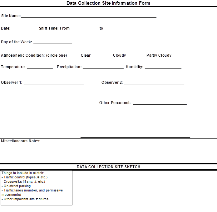
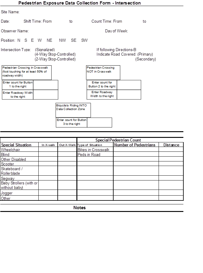
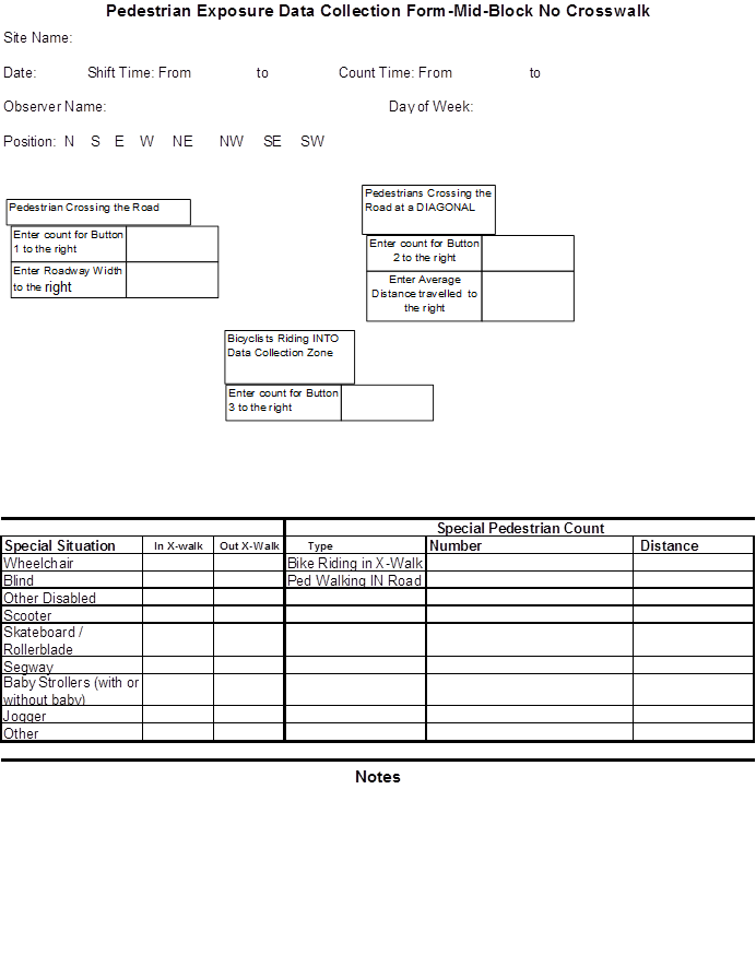
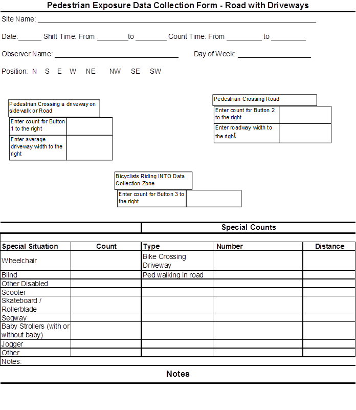
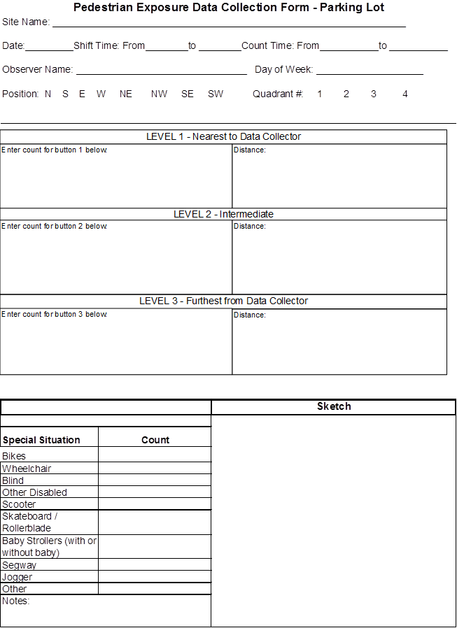
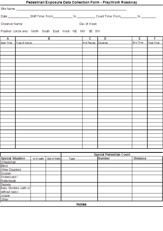
To calculate pedestrian exposure distance for a 15-min period by an observer, refer to table 11 when using the following steps and example:
Table 11. Example for one location during a 15-min pedestrian count.
| Location | Time | Observer | Pedestrians Crossing in the Crosswalk | Unit Distance Exposure (ft) | Subtotal | Pedestrians Not Crossing in the Crosswalk | Unit Distance Exposure (ft) | Subtotal | Pedestrian Count | Total Pedestrian Exposure Distance During Count Interval (ft) |
|---|---|---|---|---|---|---|---|---|---|---|
15th Street and L Street NW |
10:30-10:45 a.m. |
1 |
78 |
60 |
4,680 |
10 |
60 |
600 |
88 |
5,280 |
10:30-10:45 a.m. |
2 |
164 |
60 |
9,840 |
18 |
60 |
1,080 |
182 |
10,920 |
1 ft = 0.305 m
To calculate bicyclist exposure distance for a 15-min period by an observer, refer to table 12 when using the following step and example:
Table 12. Example for one location during a 15-min bicyclist count.
| Location | Time | Observer | Bicyclists in Roadway in Data Collection Zone | Exposure Distance (ft) | Total Bicyclist Exposure Distance During Count Interval (ft) |
|---|---|---|---|---|---|
15th Street and L Street NW |
10:30-10:45 a.m. |
1 |
7 |
50 |
350 |
10:30-10:45 a.m. |
2 |
3 |
50 |
150 |
1 ft = 0.305 m
Columns 10 and 11 from table 11 and columns 5 and 6 from table 12 are used for procedures 2A and 2B below. The pedestrian data are used for table 13, and the bicyclist data are used for table 14.
To calculate pedestrian hourly estimates (counts and exposure distance) at each signalized intersection location, refer to table 13 when using the following steps and example:
Example for Observer 1 (Primary Estimation Method)
Table 13. Example for one location to calculate pedestrian hourly estimates.
Location |
Time |
Observer |
15-min Pedestrian Count |
15-min Pedestrian Exposure Distance (ft) |
Hourly Pedestrian Count |
Hourly Pedestrian Exposure Distance (ft) |
|---|---|---|---|---|---|---|
15th Street and L Street NW |
10:30-10:45 a.m. |
1 |
88 |
5,280 |
1,080 |
64,800 |
10:30-10:45 a.m. |
2 |
182 |
10,920 |
1 ft = 0.305 m
The steps listed above apply to a majority of signalized intersections. However, a small set of locations were estimated with a slight modification as a result of different data collection methodologies employed. If counts were conducted by two observers twice within 1 h (two 15-minute counts were taken, with one count per half hour), multiply each observer's 15-min count by 2 and then add them together.
To calculate bicyclist hourly estimates (counts and exposure distance) at each signalized intersection location, refer to table 14 when using the following steps and example:
Example for Observer 1 (Primary Estimation Method)
Table 14. Example for one location to calculate bicyclist hourly estimates.
Location |
Time |
Observer |
15-min Bike Count |
15-min Bike Exposure (ft) |
Hourly Bike Count |
Hourly Bike Exposure (ft) |
|---|---|---|---|---|---|---|
15th Street and L Street NW |
10:30-10:45 a.m. |
1 |
7 |
350 |
40 |
2,000 |
10:30-10:45 a.m. |
2 |
3 |
150 |
1 ft = 0.305 m
The hourly totals for pedestrian counts and exposure distance from procedure 2A are used to estimate 24-h pedestrian volume and exposure distance described in procedure 3. The hourly total volume of pedestrians (1,080) and pedestrian exposure distance (64,800 ft (19,764 m)) represent hour 10 and are used in table 15. For hour 9, the values in columns 6 and 7 of table 13 are 1,472 and 88,320 ft (448.96 and 26,937.6 m), respectively.
To calculate pedestrian hourly estimates (volumes and exposure distance) at each signalized intersection location, refer to table 15 when using the following steps and example:
Table 15. Example of one location to estimate 24-h exposure distance and pedestrians counts.
| Hour | Factor (percent) | Exposure (ft) | Pedestrians |
|---|---|---|---|
0 |
1.7076 |
22,804 |
380 |
1 |
1.2978 |
17,331 |
289 |
2 |
0.4440 |
5,929 |
99 |
3 |
0.1025 |
1,368 |
23 |
4 |
0.0512 |
684 |
11 |
5 |
0.1537 |
2,052 |
34 |
6 |
0.8623 |
11,516 |
192 |
7 |
4.8893 |
65,292 |
1,088 |
8 |
7.8221 |
104,457 |
1,741 |
9 |
5.8264 |
88,320 |
1,472 |
10 |
5.6398 |
64,800 |
1,080 |
11 |
4.8341 |
64,555 |
1,076 |
12 |
5.6095 |
74,910 |
1,248 |
13 |
6.9955 |
93,419 |
1,557 |
14 |
7.3010 |
97,498 |
1,625 |
15 |
6.3995 |
85,459 |
1,424 |
16 |
12.1326 |
162,020 |
2,700 |
17 |
10.0078 |
133,645 |
2,227 |
18 |
3.6884 |
49,256 |
821 |
19 |
6.6021 |
88,164 |
1,469 |
20 |
1.3226 |
17,662 |
294 |
21 |
1.4947 |
19,960 |
333 |
22 |
1.8101 |
24,172 |
403 |
23 |
3.0054 |
40,134 |
669 |
Total |
1,335,407 |
22,257 |
|
1 ft = 0.305 m Note: Bold indicates hours for which actual data were collected.
Steps 3 and 4 of procedure 3 show an example of how one row in table 15 is filled in. Hour 0 is used as an example as follows:
The remaining hours should be filled for hourly pedestrian volume and exposure distance by also using steps 3 and 4, respectively.
The 24-h totals for pedestrian counts and exposure distance from procedure 3 are used to estimate annual counts and exposure distance in procedure 4A. The 24-h total of pedestrians (22,257) and exposure distance (1,335,407 ft (407,299 m)), along with the totals from the other 38 signalized intersections, are used to calculate the geometric mean for all signalized intersections. This geometric mean is used in procedure 4A to estimate annual pedestrian volumes and exposure distance for that facility type for the entire city.
To calculate annual pedestrian estimates (counts and exposure distance) at all signalized intersection locations, refer to table 16 when using the following steps and example:
Table 16. Example of estimates of pedestrian counts and distance for one location type (signalized intersection) for an entire city.
| Facility Type (n) | Number of Facilities | Volume (Geometric Mean) | Distance (ft) (Geometric Mean) | Annual Pedestrian Volume (millions) | Annual Pedestrian Distance (millions of mi) |
|---|---|---|---|---|---|
Signalized intersection (39) |
1,581 |
2,403 |
127,552 |
1,373 |
13.8 |
n = Sample size 1 ft = 0.305 m 1 mi = 1.61 km
To calculate annual bicyclist estimates (counts and exposure distance) at all signalized intersection locations, refer to table 17 when using the following steps and example:
Table 17. Example of estimates of bicyclist counts and distance for one location type for an entire city.
| Facility Type (n) | Number of Facilities | Volume (Geometric Mean) | Distance (ft) (Geometric Mean) | Annual Bicyclist Volume (millions) | Annual Bicyclist Distance (millions of mi) |
|---|---|---|---|---|---|
Signalized intersection (39) |
1,581 |
319 |
159,694 |
184 |
17.5 |
n = Sample size 1 ft = 0.305 m 1 mi = 1.61 km
FHWA sponsored this work. This research could not have been completed without the assistance and advice of numerous people, including the following FHWA contractors and government employees: Elliott Tibor, Sheryl Miller, Gabriel Rousseau, Dana Duke, Vernese Edghill, Wanda Parham, Tiana Petit, Megan Hermosillo, Erin Dagnall, and Mary Carolyn Thies. George Branyan, Bill McGuirk, and Yusuf Aden from DDOT were valuable resources during the planning and data collection phases of the study. Stephen Fleger as well as Thomas Granda and Christopher Monk (FHWA) managed the overall support services contract under which the work was performed.
1. National Center for Statistics and Analysis. (2009). Traffic Safety Facts: 2008 Data, Report No. DOT HS 811 162, National Highway Traffic Safety Administration, Washington, DC.
2. National Highway Traffic Safety Administration. (2009). Fatality Analysis Reporting System, Washington, DC. Obtained from: http://www-fars.nhtsa.dot.gov/Main/index.aspx. Site last accessed September 30, 2009.
3. National Highway Traffic Safety Administration. (2009). National Automotive Sampling System General Estimates System, Washington, DC. Obtained from: http://www.nhtsa.gov/NASS. Site last accessed September 30, 2009.
4. Office of Highway Policy Information. (2007). Highway Statistics 2006, Federal Highway Administration, Washington, DC.
5. Hedlund, J. (2000). NHTSA/FHWA Pedestrian and Bicycle Strategic Planning Research Workshops, Highway Safety North, Ithaca, NY.
6. Rodgers, G.B. (1994). "The Characteristics and Use Patterns of Bicycle Riders in the United States," Journal of Safety Research, 25, 83-96.
7. Jacobsen, P.L. (2003). "Safety in Numbers: More Walkers and Bicyclists, Safer Walking and Bicycling," Injury Prevention, 205-209.
8. Ivan, J., Ossenbruggen, P.J., Qin, X., and Pendarkar, J. (2000). Rural Pedestrian Crash Rate: Alternative Measures of Exposure, University of Connecticut, Storrs, CT.
9. Silcock, D.T., Walker, R., and Selby, T. (1996). Pedestrians at Risk, 1-12, PTRC 24th European Transport Conference, Brunel University, Uxbridge, London.
10. Zegeer, C.V., Stewart, J.R., Huang, H.H., Lagerwey, P.A., Feaganes, J., and Campbell, B.J. (2005). Safety Effects of Marked Versus Unmarked Crosswalks at Uncontrolled Locations: Final Report and Recommended Guidelines, Report No. FHWA-HRT-04-100, Federal Highway Administration, Washington, DC.
11. Cameron, M.H. and Milne, P.W. (1978). Pedestrian Exposure and Risk in New South Wales, Joint ARRB/DOT Pedestrian Conference, Sydney, Australia.
12. Davis, S., King, E., Robertson, D., Mingo, R., and Washington, J. (1987). Measuring Pedestrian Volumes and Conflicts Volume I: Pedestrian Volume Sampling, Final Report, Analysis Group, Inc., Washington, DC.
13. Tobey, H.N., Shunamen, E.M., and Knoblauch, R.L. (1983). Pedestrian Trip Making Characteristics and Exposure Measures, Center for Applied Research, Inc., Great Falls, VA.
14. Keall, M.D. (1995). "Pedestrian Exposure to Risk of Road Accident in New Zealand," Accident Analysis and Prevention, 27, 729-740.
15. Chu, X. (2003). The Fatality Risk of Walking in America: A Time-Based Comparative Approach, 4th International Conference on Walking in the 21st Century, Portland, OR.
16. Bly, P., Dix, M., and Stephenson, C. (1999). Comparative Study of European Child Pedestrian Exposure and Accidents, MVA Limited, Surrey, England.
17. Bureau of Transportation Statistics. (1998). Walking in Great Britain, London, England.
18. Kaplan, J.A. (1975). Characteristics of the Regular Adult Bicycle User, 132, University of Maryland College Park, College Park, MD.
19. Molino, J., Kennedy, J., Johnson, P., Beuse, P., Emo, A., and Do, A. (2009). "Pedestrian and Bicyclist Exposure to Risk," Transportation Research Record 2140, 145-156, Transportation Research Board, Washington, DC.
20. The District of Columbia. DC Area-DDOT Traffic Camera Location Map, District Department of Transportation, Washington, DC. Obtained from: http://app.ddot. dc.gov/services_dsf/traffic_cameras/index.asp. Site last accessed September 30, 2009.
21. ESRI®. (2007). ArcGIS, Version 9.1, Redlands, CA.
22. AT&T. Yellow Pages, Glendale, CA. Obtained from: www.yellowpages.com. Site last accessed February 28, 2008.
23. DC Public Schools. DC Public Schools Directory, Washington, DC. Obtained from: http://profiles.dcps.dc.gov/ Site last accessed May 24, 2011.
24. SAS Institute, Inc.®. (1999). SAS/STAT, Version 8, Cary, NC.
25. DC Office of the Chief Technology Officer. Existing Land Use Map, The District of Columbia, Washington, DC. Obtained from: http://planning.dc.gov/DC/Planning/ DC+Data+and+Maps/Map+Library/Existing+Land+Use+Map. Site last accessed May 23, 2011.
26. The Old Farmer's Almanac, (2008). Dublin, NH. Obtained from: www.almanac.com/ astronomy. Site last accessed July 15, 2008.
27. Osborne, J. (2002). "Notes on the Use of Data Transformations," Practical Assessment, Research and Evaluation, 8. Obtained from: http://pareonline.net/getvn.asp?v=8&n=6. Site last accessed July 15, 2009.
28. Destination DC. (2007). Washington DC's 2006 Visitor Statistics, Washington, DC. Obtained from: http://www.washington.org/images/marketing/2006_visitorstats.pdf. Site last accessed August 4, 2009.
29. U.S. Census Bureau. (2009). District of Columbia Quickfacts, Washington, DC. Obtained from: http://quickfacts.census.gov/qfd/states/11000.html. Site last accessed May 24, 2011.
30. Destination DC. (2008). Washington DC's 2007 Visitor Statistics, Washington, DC. Obtained from: http://washington.org/images/marketing/2007_visitor_statistics_final.pdf. Site last accessed May 5, 2010.
31. Christie, L. (2005). "Biggest Commuter Cities," CNN Money, Atlanta, GA. Obtained from: http://money.cnn.com/2005/10/21/real_estate/buying_selling/daytime_population_cities/. Site last accessed May 24, 2011.
32. Goodwin, P.B. and Hutchinson, T.P. (1977). "The Risk of Walking," Transportation, 6, 217-230.
33. Radford, N. and Ragland, D. (2004). "Space Syntax: Innovative Pedestrian Volume Modeling Tool for Pedestrian Safety," Transportation Research Record 1878, 66-74, Transportation Research Board, Washington, DC.


 intersection. This photo shows an example of a stop-controlled (all-way intersection). The intersection is a four-way intersection with stop signs at all sides. There are sidewalks and trees on all sides of the road.")
 intersection. This photo shows an example of a partially stop-controlled (one- or two-way) intersection. There is a four-way intersection with four crosswalks. One stop sign is visible on the right-hand side. There are buildings and sidewalks on all sides of the intersection.")
 intersection data collection configuration. This photo shows an aerial view of the areas of responsibility for two data collectors for a signalized and stop-controlled intersection. It is a four-way intersection with four crosswalks. The areas of responsibility for two data collectors are sectioned by color. There is a red circle labeled 1 at the top left side of the intersection and a blue circle labeled 2 diagonally across from it at the bottom right side of the intersection. There is a red outline around the top and right side of the intersection to indicate the area that the first collector should observe. There is a blue outline around the bottom and left side of the intersection to indicate the area that the second collector should observe.")
 intersection data collection configuration. This photo shows an aerial view of a partially stop-controlled (one- or two-way) intersection. It is a four-way intersection with four crosswalks. The areas of responsibility for two data collectors are sectioned by color. There is a red circle labeled 1 at the top left side of the intersection and a blue circle labeled 2 diagonally across from it at the bottom right side of the intersection. A red box marked primary encompasses the vertical street, including the middle of the intersection, indicating the area that the first collector should observe. There are two blue boxes on the horizontal street on either side of the red box and are marked secondary, indicating the area that the second collector should observe. The length of each blue box is 50 ft (15.25 m).")


 and a bottom section (outlined in green). Both the top and bottom are further divided into three vertical sections labeled A, B, and C.")


 in blue and Zegeer et al. in red. The blue line is below the 2 percent adjustment factor level for the first 7 hours and then trends up to account for the morning commute at hour 8 to about 8 percent. A small dip occurs during the lunch hours (hours 11 and 12), followed by a high upward trend in the evening commute hours (between hours 16 and 17). The peak of the curve occurs at 12 percent. A small peak occurs at hour 19, followed by a significant drop off from hour 20 to 23. The plot of the red line is similar to the blue line. However, during the midday periods, there is more of an upward trend between hours 9 and 12. The highest adjustment factor peak for the red line occurs at hour 15 at slightly higher than 10 percent.")
. The line has a flat profile at the early hours of the day, with the data at or slightly above 0 percent between the hours 0 and 5. A large upward trend occurs between hours 6 and 8, with a peak adjustment factor of over 22 percent. A sharp decline occurs, and there is a fairly flat plateau between the hours 9 and 19, with adjustment factors between 4 and 6 percent. The line falls below 5 percent between hours 20 and 23.")

. The bar graph shows frequency on the y-axis from zero to 25 in increments of 5 and the natural log of estimated daily pedestrian counts on the x-axis from zero to 12 in increments of 2. The mean equals 6.73, the standard deviation equals 1.848, and N equals 122. The graph has a peak proportion in the middle of the graph, with the data dropping off on both sides of the peak. The transformed data are close to a normal distribution, and the overall data resemble a bell curve.")

 pedestrian counts to estimated counts using the phase II technique with DDOT data. Actual DDOT daily pedestrian counts with natural logarithmic transformation is on the y-axis from 4 to 12 in increments of 1. Federal Highway Administration estimate of DDOT daily pedestrian counts with natural logarithmic transformation is on the x-axis from 4 to 12 in increments of 1. The three trendlines (linear first hour estimate, linear second hour estimate, and linear perfect prediction) start in the lower left and increase to the upper right at around a 45-degree angle from the x-axis. The trendlines are in close proximity to each other and follow a similar pattern. The data points (first hour estimate, second hour estimate, and average estimate) are on or very close to the trendlines and are near the middle and/or ends of the trendlines.")
 pedestrian counts to estimated counts using the phase II technique with Federal Highway Administration (FHWA) data. Actual DDOT daily pedestrian counts with natural logarithmic transformation is on the y-axis from 4 to 12 in increments of 1. FHWA estimate of FHWA daily pedestrian counts with natural logarithmic transformation is on the x-axis from 4 to 12 in increments of 1. The three trendlines (linear first hour estimate, linear second hour estimate, and linear perfect prediction) start in the lower left and increase to the upper right at around a 45-degree angle from the x-axis. The trendlines are in close proximity to each other. The data points (first hour estimate, second hour estimate, and average estimate) are on or very close to the trendlines and are near the lower end of the trendlines.")