• Federal Highway Administration >
• Publications >
• Research Publications >
• 98107 >
• Section4.Cfm >
• Capacity Analysis of Pedestrian and Bicycle Facilities

Capacity Analysis of Pedestrian and Bicycle Facilities

Recommended Procedures for the "Pedestrians" Chapter of the Highway Capacity Manual

PDF Version (596 KB)

4. METHODS FOR COMPUTING MEASURES OF EFFECTIVENESS

Note: All values for walking speeds are those used by the original researcher, rather than those recommended in this report, unless otherwise noted.

4.1 Uninterrupted Facilities

Sidewalks and Walkways

The existing HCM contains detailed analysis procedures for these facilities (TRB, 1994). Although this report recommends new LOS thresholds, the basic procedures for the facilities will not change.

Off-Street Paths

Exclusive Pedestrian Trails. As stated earlier, the existing HCM procedures for walkway analysis apply here. Although this study recommends new service level thresholds, the basic procedure for these facilities will not change.

Shared Pedestrian-Bicycle Paths. For these facilities, Botma's procedure, described earlier, is the only viable alternative in the literature. The procedure consists of measuring bicycle volume and then assigning a pedestrian LOS based on this volume.

4.2 Interrupted Pedestrian Facilities

Signalized Crossings

The existing HCM contains detailed analysis procedures for these facilities (TRB, 1994). Chapter 13 notes that one can analyze a crosswalk as a time-space zone, similar to a street corner. According to the HCM, the demand for space equals the product of pedestrian crossing flow and average crossing time. The chapter notes that a surge condition exists when the two opposing platoons meet. One determines the primary measure of effectiveness, space per pedestrian, using this time-space methodology. No delay measures exist, as stated earlier.

Delay: Pretty's Method. Pretty (1979) analyzed the delays to pedestrians at signalized intersections using relatively simple models. For pedestrians crossing one street at an intersection, he developed the following formula for pedestrian delay, based on uniform arrival rates and equal pedestrian phases:

where:

For pedestrians crossing two streets at an intersection, he offers the following formula, which assumes that one-half the cycle length separates the two WALK periods:

where:

For an all-pedestrian phase, sometimes referred to as a "barn dance" or "Barnes dance," the total pedestrian delay is of the same form as that for a single crossing:

where:

Delay: Dunn and Pretty's Method. Dunn and Pretty (1984) determined the following formulas for pedestrian delay at signalized pedestrian (Pelican) crossings:

	for a narrow roadway (about 7.5 m or two lanes)
	for a wider roadway (about 15 m or four lanes)

where:

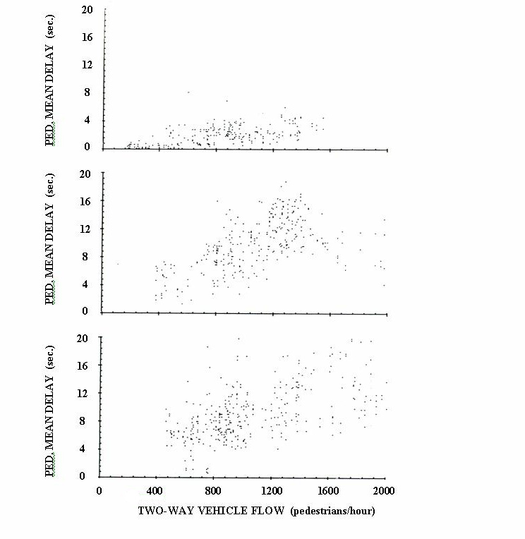
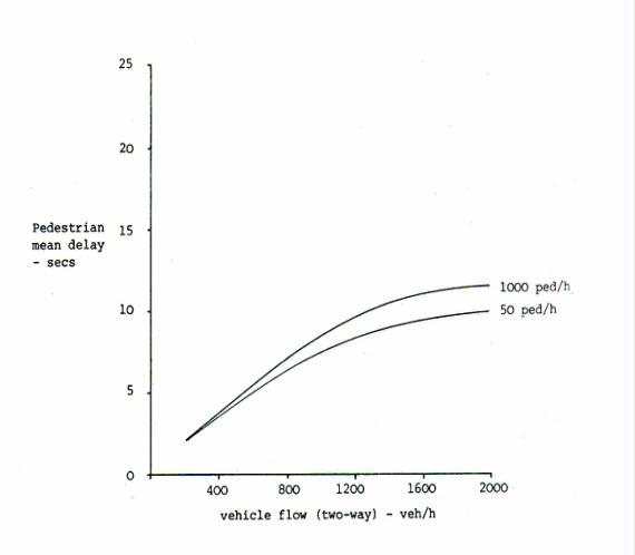
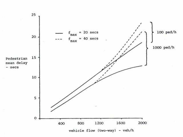
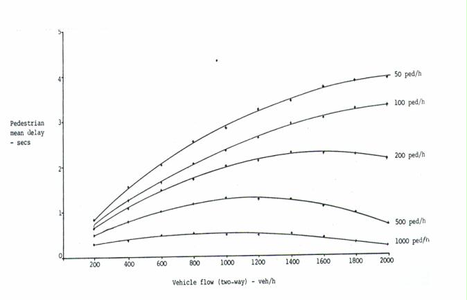
The parenthetical expressions in the denominator represent the cycle length for the above expressions, which assume pedestrian signal compliance.

Delay: Griffiths et al.'s Method. Griffiths et al. (1984a) conducted field surveys of delay at midblock pedestrian crossings in Great Britain. Figure 9 shows the results of the authors' field study. The top graph represents zebra crossings. The middle graph represents fixed-time pelican crossings. The lower graph represents vehicle-actuated pelican crossings.

As mentioned earlier, Griffiths et al. (1984c) performed extensive simulation analyses on a 10-m-wide pelican crossing. The authors found an increase in pedestrian delay with increases in vehicle flow, because the former group enjoys reduced opportunities to cross in gaps in traffic under higher vehicle flow conditions. The authors found a moderate increase in pedestrian delay with increases in pedestrian flow. Under vehicular actuation, the authors found that an increase in vehicular green from 20 to 40 s (in response to higher vehicle flows) resulted in rapid increases in pedestrian delay above two-way flows of 1,000 veh/h but no change in pedestrian delay below these levels.

Figures 10 and 11 graphically depict the results of their simulation analyses on pelican crossings. Figure 10 refers to a fixed-time pelican crossing with a vehicle precedence period (f_max) of 20 s. Figure 11 shows a vehicle-actuated pelican crossing, with the solid lines representing f_max = 20 s and the dashed line representing f_max = 40 s. The latter figure shows the effect of increasing pedestrian flow on pedestrian delay at higher vehicle flows.

This report has also mentioned that Griffiths et al. (1985) developed mathematical expressions for delay at fixed-time signal crossings. The appendix describes these formulas.

Delay: Roddin's Method. Roddin (1981) offers the following equation for average delay (D) to pedestrians at signalized intersections:

where:

Roddin assumes random pedestrian crossings during WALK and random vehicle arrivals throughout the cycles.

FIGURE 9: Field Measurements of pedestrian delay at midblock crossings in Great Britain.
SOURCE: Griffiths et al., 1984a.

FIGURE 10: Simulation results of pedestrian dealy at fixed-time Pelican crossings in Great Britain.
SOURCE: Griffiths et al., 1984c.

FIGURE 11: Simulation results of pedestrian delay at vehicle-actuated Pelican crossings in Great Britain.
SOURCE: Griffiths et al., 1984c.

Delay: Virkler's Method. Virkler clearly states that "pedestrians can save significant amounts of delay by using more than just the WALK interval to enter the intersection." He develops a new model of pedestrian delay that reflects the benefits of noncompliance on pedestrian delay:

where:

Virkler applied this equation to actual measured delay at 18 Brisbane, Australia, crosswalks and found that the equation predicted delay about 1 percent higher than observed values.

Delay: NCSU's Method. Gerlough and Huber (1975) discuss several intersection delay and queueing models for vehicles. They derive a fluid (or continuum) delay model for a pretimed signal, and then note that this formulation is identical to the first term of the famous Webster analytical model for computing delay. One can write this portion of the model as:

where:
	d = delay, s;
	C = cycle length, s;
	g = effective green time, s;
	x = q C / (g s);
	q = arrival rate on approach, ped/h; and
	s = saturation flow rate on approach per/hour green.

The NCSU research team observed flow rates up to 5,000 ped/h ped-green at some locations. Inserting this value for the maximum pedestrian saturation flow rate, one has:

However, the NCSU team observed no capacity constraints, even with pedestrian flow rates of 5,000 ped/h. Therefore, rather than substitute this value for a maximum saturation flow rate, one could alternatively assume that the maximum saturation flow rate(s) approaches infinity for pedestrians. In this case, the term in brackets {1 – q/s} will tend to unity as s approaches infinity, and the following simple formula remains:

This last expression is identical to that found in the Australian Road Research Board Report 123 for pedestrian delay (Akçelik, 1989).

Space. The HCM contains a detailed analysis procedure for determining the space measure of effectiveness for pedestrians for signalized crossings. Although the general time-space framework appears sound, several researchers have noted problems associated with particular aspects of the procedure. These areas include street corner waiting areas, corner circulation times, start-up times, and minimum crossing times.

Space: Fruin, Ketcham, and Hecht's Method. Fruin, Ketcham, and Hecht (1988) recommend several changes to the HCM method based on time-lapse photographic observations of Manhattan Borough, New York City, street corners and crosswalks. First, they advocate the use of 7 ft²/person (about 0.65 m²/person) for standing area on a street corner, rather than the HCM value of 5 ft²/person (0.46 m²/person). They also recommend a change in corner circulation time from a constant of 4 s to the following formula based on corner dimensions:

where:

where:

Space: Virkler Methods. Virkler, Elayadath, and Geethakrishnan (1995) note that the signalized intersection chapter of the HCM, among other references, contains a basic crossing time (T) equation of the following general form:

Virkler and Guell (1984) provide a method for determining intersection crossing time (T) that incorporates platoon size:

Virkler, Elayadath, and Geethakrishnan (1995) note that the Virkler and Guell equation does not address the problem of opposing platoons meeting in a crosswalk. In addition, these authors state that the current HCM time-space methodology suffers from two flaws dealing with the available time-space and walking time. Concerning the former, Virkler et al. (1996) believe that the HCM methodology overestimates the available time-space by about 20 percent, because legally crossing pedestrians cannot reach the space in the center of the crosswalk at the beginning of the phase and must have cleared this space by the end of the phase. Regarding the latter, Virkler et al. note that the time-space product ignores the fact that pedestrians must have sufficient time to physically traverse the entire length of the crosswalk. They imply that one should subtract the quotient of the crosswalk length and twice the assumed walking speed from the crosswalk time-space product for accuracy.

Those authors advocate the use of an approach based on shockwave theory when crossing pedestrian platoons are large, perhaps seven pedestrians per platoon (very roughly, 300 per hour). The shockwave assumptions include: opposing platoons occupy the full walkway width until they meet and one-half of the walkway width upon meeting, pedestrian speeds fall upon meeting and remain low after platoon separation, and pedestrian density increases at platoon meeting. The Appendix contains the expression for required effective green time from Virkler et al. This model implies that, for a 60-s cycle length and a 30-s effective green time, 1,000 ped/h in the major direction would result in inadequate crossing time for crosswalk lengths greater than about 16 m despite an average LOS of B and a surge LOS of C. In addition, 250 ped/h in the major direction would have inadequate time for crosswalk lengths above 27 m, even with a surge LOS of A.

More recently, Virkler conducted a study in the Brisbane, Australia, area to determine appropriate crossing time parameters for two-way and scramble (all-pedestrian phase) crosswalk flow (Virkler, 1997c). Virkler notes that, for both types of facilities, the width of crosswalk actually used by pedestrians increases with increasing crosswalk volume. As mentioned earlier, Virkler also states that vehicles often use a portion of the crosswalk during the pedestrian phase. He therefore cautions that engineers should treat measured crosswalk widths merely as the width "intended for pedestrian use" rather than as an exact measurement of the width pedestrians will actually use. As an aside, Pretty argued against the use of exclusive pedestrian phases because of the considerable increase in pedestrian delay (Pretty et al., 1994).

As mentioned in the Literature Review for Chapter 13, Pedestrians, of the Highway Capacity Manual, Virkler (1997c) found that speeds at the rear of the platoons are not independent of concurrent or opposing platoon sizes. He found that, with large platoon sizes, the typical 7-s WALK interval is insufficient to allow all pedestrians to enter the crosswalk. For platoons of about 15 people or more, he states that the engineers should extend the minimum crossing time on a typical 3-m-wide crosswalk by 0.27 s/ped headway plus 1.71 s. The Appendix contains these calculations.

Unsignalized Crossings
The existing HCM contains no procedures for analyzing these facilities.

Delay: Roddin's Method. Roddin (1981) describes a method by another researcher for calculating moderate (less than 18 s) mean pedestrian delay (D) at unsignalized intersections:

Delay: Virkler's Method. Virkler (1996) describes a similar equation for calculating delay from other research, based on queueing theory. Assuming random vehicle arrivals and normal crossing speeds, the expression is:

Delay: Griffiths' et al.'s Method. As described earlier, Griffiths et al. (1984b) performed extensive simulation analysis on zebra crossings. They found that pedestrian delay depends heavily on both pedestrian and vehicle flows; however, they noted that the effect of increasing vehicle flow occurs primarily at low pedestrian volumes. In fact, as vehicle volumes continue to increase, pedestrian delay actually decreases, because most vehicles begin from a stopped (queued) position and pedestrians can establish precedence easier. Figure 12 depicts the authors' field results.

FIGURE 12: Simulation results of pedestrian delay at Zebra crossings in Great Britain.
SOURCE: Griffiths et al., 1984b.

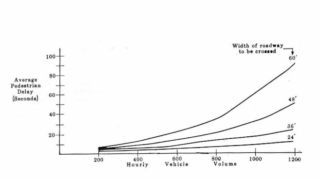
This report has also mentioned that these same authors developed mathematical delay models. The Appendix contains the expression developed by Griffiths et al. for pedestrian delay at a zebra crossing.

Smith Method. Smith et al. (1987) refer to an earlier study that demonstrated the effect of crossing width and conflicting vehicle volume on pedestrian delay (Figure 13).

Palamarthy Method. Palamarthy et al. (1994) present the following model for mean pedestrian delay for all pedestrians employing one of the crossing tactics mentioned earlier in the discussion of unsignalized service measures of effectiveness:

where:
	di = mean delay to pedestrians using tactic i, s per pedestrian;
	q = vehicular flow in one direction, vehicles/s;
	"n = critical gap in near-lane traffic stream, s; and
	"f = critical gap in far-lane traffic stream, s.

It follows that the mean delay across all tactics is:

where:
	d = mean delay to all crossing pedestrians, s/pedestrian; and

FIGURE 13: Effect of crossing width and conflicting vehicle volume on pedestrian delay.
SOURCE: Smith et al., 1987.

NCSU's Method. The NCSU research team has developed a formulation for computing pedestrian delay at unsignalized intersections based on gap acceptance by platoons. Since "delays are relatively insensitive to the form of the distribution of the arriving traffic" (Gerlough and Huber, 1975), the research team assumed random arrivals for both pedestrians and vehicles. In addition, the procedure described in the following paragraphs assumes that start-up times, headways, walking speeds, and minimum pedestrian body ellipses retain constant values. The ITE Manual of Traffic Engineering Studies (Robertson et al., 1994) contains a general equation describing the minimum safe gap (G) in traffic:

Gerlough and Huber (1975) note that, for a group of pedestrians, the pedestrian and vehicle volume together determine the size of the platoon:

where:
	E(nc) = size of typical pedestrian crossing platoon, ped;
	p = pedestrian flow rate, ped/h;
	q = vehicular flow rate, veh/h;
	= critical gap or minimum "intervehicular spacings"

One can make an estimate of a critical gap, , for a single pedestrian by substituting N = 1 into the ITE equation above and simplifying:

Then, one substitutes this value for critical gap,,into the Gerlough and Huber expression above to determine the number of pedestrians in a typical crossing platoon. To determine the spatial distribution of pedestrians, the research team developed a simple geometric expression incorporating the crosswalk width and the pedestrian body buffer zone:

crosswalk width

As stated earlier, the research team recommends a value of 0.75 m² for a design body buffer zone. Given the critical gap for a single pedestrian computed previously, the ITE equation simplifies to:

The ITE Manual suggests 2 s as a typical value of headway, H. To avoid confusion, this report will refer to the pedestrian group critical gap (G in the previous equation) as _G . The final issue concerns the average delay to all pedestrians, whether waiting or not. Again, Gerlough and Huber (1975) provide guidance:

where:
	E(t) = average delay to all pedestrians, s;
	T = 1/q = mean vehicle headway, 1/s; and

Other Waiting Areas

Space. The existing HCM does not contain detailed analysis procedures for waiting areas, because the methodology is extremely simple. One simply computes the available waiting area and determines the actual or expected number of pedestrians during the critical time period, and then determine the LOS from the average space per pedestrian. Fortunately, queueing areas sufficiently resemble street corners such that one can apply those procedures if needed.

4.3 Pedestrian Networks

Travel Time: Roddin's Method. Roddin (1981) mentions one quantitative factor, travel time, in the evaluation of pedestrian transportation. His narrative implies that the following equation applies to pedestrian networks:

Travel Time: Virkler's Method. Virkler (1997b) provides an extensive method of calculating travel time along a pedestrian network. Incorporating both link and note components, his methodology determines the total walking plus queueing time along the extended pedestrian facility. For congruence with vehicle arterial measures of effectiveness, the method determines the average travel speed along the route as a final step.

Virkler notes that platooning due to an upstream signal can either increase or decrease pedestrian delay at a downstream signal, depending on the offset and the green time at the upstream signal (1997d). He argues that one can use field measurements of arrival patterns at signals to modify random arrival-based delay results. Table 24 shows his recommended default delay adjustment factors (DFs) to achieve positive pedestrian platooning.

Examination of the table demonstrates that DF between 0.45 and 0.64 lie within the likely range at all listed green time/cycle length ratios. In addition, the table demonstrates that one will achieve better (lower) delay adjustment factors at higher green ratios (g/C). He notes that the best offsets for pedestrian progression do not necessarily occur when one achieves the highest arrival rate during the green; rather, one must consider the green time itself. Virkler found that, as green times increase, the best offsets are shorter, in order to maximize the benefits of pedestrian platooning.

TABLE 23 Default values of Delay Adjustment Factors (DF) for positive pedestrian platooning.

The Federal Highway Administration is dedicated to providing alternative formats of information and publications that are accessible to people with disabilities. For additional information or to request an alternative format, please send an e-mail to: TFHRC.WebMaster@fhwa.dot.gov