


- Highway Sensitivity Analysis
- Alternative Growth Rates in Prices and Travel Demand
- Alternative Rates of Growth in Travel Demand—HERS
- Alternative Rates of Growth in Travel Demand—NBIAS
- Alternative Forecasts of Fuel Prices and Vehicle Fuel Efficiency—HERS
- Construction Cost Indices—HERS
- Alternative Economic Analysis Assumptions
- Value of a Statistical Life
- Value of Ordinary Travel Time
- Value of Incident Delay Reduction—HERS
- Elasticity Values—HERS
- Discount Rate
- High-Cost Transportation Capacity Investments
- Alternative Growth Rates in Prices and Travel Demand
- Transit Sensitivity Analysis
Highway Sensitivity Analysis
The results produced by the Highway Economic Requirements System (HERS), the National Bridge Investment Analysis System (NBIAS), and the Transit Economic Requirements Model (TERM) reflected in the investment scenario estimates presented in this report are strongly affected by the values of certain key variables. In any modeling effort, it is critical to evaluate the validity of the underlying assumptions and determine the degree to which projected outcomes could be affected by changes to these assumptions. (Note that the analyses presented in this section relate primarily to technical assumptions; Chapter 9 includes similar analyses of some more policy-oriented assumptions, including the rate of deployment of operations strategies, the implementation of congestion pricing, and the adoption of alternative bridge management strategies.)
This section explores the sensitivity of the HERS and NBIAS projections from Chapter 7 to variation in some of the underlying assumptions. These sensitivity analyses pertain to the types of capital projects within the current scopes of the HERS and NBIAS models—pavement and system expansion projects on Federal-aid highways, and all bridge system rehabilitation projects, respectively. Excluded from analysis are pavement or system expansion improvements to other roads, or any system enhancements such as safety, traffic operational, or environmental enhancements; these types of highway capital improvements are not currently directly modeled in HERS or NBIAS. Sensitivity analyses are conducted separately for HERS and NBIAS; the results obtained from the two models were not combined.
It is important to note that the analyses for highways and bridges presented in this chapter relate to individual scenario components only, rather than to complete scenarios, so that the investment levels shown in the various exhibits are not directly comparable to those presented in Chapter 8. In order to fully reconstruct a Chapter 8 scenario using input from this section, one would need to combine a modified HERS-derived component with a modified NBIAS-derived component and to re-estimate the nonmodeled component of the scenario in the manner described in Chapter 8.
The first part of this section considers the uncertainty surrounding future trends in traffic volumes, fuel prices and vehicle fuel efficiency; and changes in construction costs. The second part includes additional sensitivity tests of the assumptions in the HERS and NBIAS simulations. These tests vary the assumptions about the value travelers attach to reductions in travel time and crash risk, the sensitivity of travel demand to changes in the cost of travel, and the discount rate used to convert future costs and benefits into present equivalents. An additional test drops the options normally included in HERS for adding capacity to a highway section through high-cost means (such as tunneling or double-decking) when the Highway Performance Monitoring System (HPMS) database indicates that conventional widening is infeasible. A subsequent section within this chapter explores information regarding the assumptions underlying the analyses developed using TERM.
Alternative Growth Rates in Prices and Travel Demand
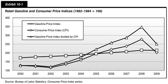
Future traffic projections, central to evaluations of capital spending on transportation infrastructure, are speculative. Fuel prices are also difficult to forecast as indicated by the historical volatility depicted in Exhibit 10-1 and by the alternate scenarios for fuel prices in the Energy Information Administration’s Annual Energy Outlook 2010. Measurement of changes in highway construction costs has become problematic in recent years as these costs have become more volatile; the diversity among highway capital improvement types and changes in data availability have added to the uncertainty in this area.
Alternative Rates of Growth in Travel Demand—HERS
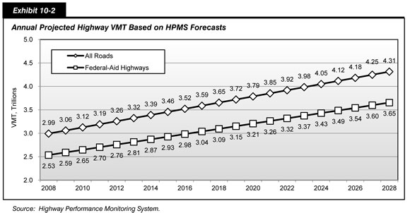
States provide forecasts of future vehicle miles traveled (VMT) for each individual HPMS sample highway section, based on available information concerning the particular section and the corridor of which it is a part. The composite weighted average annual VMT growth rate based on these forecasts is 1.85 percent. Exhibit 10-2 shows projected year-by-year VMT for 2008 to 2028 for Federal-aid highways and all roads combined. Consistent with the approach used in the HERS and NBIAS analyses for this report, the values shown assume that VMT will grow in a linear fashion (so that 1/20th of the additional VMT is added each year), rather than geometrically (growing at a constant annual rate). Under this assumption, the annual percent rate of growth gradually declines over the forecast period. Projected VMT growth in rural areas averages 2.15 percent per year, somewhat higher than the average of 1.70 percent in urban areas. The forecasts for 2008 to 2028 are lower than the actual average annual VMT growth rate of 1.94 percent that occurred from 1988 to 2008.
HERS assumes that the forecast for each HPMS sample highway segment represents the amount of travel that would occur if the level of service on that segment remained at the base-year value. To measure level of service, HERS uses average highway user cost per VMT, including costs of travel time, vehicle operation, and crash risk. The average user cost will be forecast to remain at the base year value only under specific assumptions about the level and allocation of future investment. In all other cases, projected user costs will differ from the base year value, triggering an upward or downward adjustment in projected future VMT. Generally, higher levels of investment are associated with relatively higher levels of service for the overall system, higher VMT growth, and relatively lower highway user costs. Changes in average user cost that HERS forecasts affect the travel demand projections through the demand elasticity, which measures the sensitivity of travel volumes to changes in the effective price of driving.
The effective VMT growth rates predicted by the HERS model could thus be off-target because of inaccuracies in either the forecasts of the travel that would occur under a constant level of service or the predictions of demand responses to changes in average user cost. To address the former of these potential sources of error, this section includes a sensitivity analysis that varies the annual percentage rate at which VMT is assumed to grow under a constant level of service. As alternatives to the baseline assumption of 1.85 percent per annum growth derived from the HPMS, the sensitivity analysis uses the average rates of VMT growth over the 5- and 10-year periods ending in the base year. Potential errors in the elasticity-based predictions of demand responses are addressed in a separate sensitivity analysis later in this chapter.
| What are some of the technical limitations associated with the analysis of alternative travel growth rates included in this section? | |
|
One of the strengths of the State-provided VMT forecasts used in the baseline analysis is their geographic specificity: Separate forecasts are provided for the more than 100,000 HPMS sample sections. In forming these forecasts, States can take account of specific local influences on travel growth and their own long-range planning assumptions about future travel patterns on particular routes or corridors. The inclusion of these section-level forecasts, as opposed to regional or statewide travel estimates, allows for more refined analyses of projected future investment/performance relationships.
The analyses of alternative travel growth rates presented in this section use the HPMS forecasts as a starting point, but adjust them up or down in uniform proportion on a national basis. In reality, if VMT were to grow faster or slower than State projections, these differences would not be uniform, and could be heavily concentrated in particular corridors, regions, or States. Moreover, these differences could significantly impact the level of investment that might be required to achieve particular systemwide performance targets. The assumption of uniformity thus limits the reliability of this section’s analysis of alternative VMT growth rates. |
|
During the period 1998–2008, VMT in the United States increased at an average annual rate of 1.23 percent, which is 0.62 percentage points lower than the baseline forecast. During the latter half of this period, 2003–2008, the average annual rate of increase was only 0.53 percent, reflecting the slow-down in VMT growth discussed in Chapter 2. Exhibit 10-3 shows that replacing the baseline forecast of the VMT growth rate with the lower rates that occurred in recent years reduces the HERS-based estimates of the maximum cost-beneficial amount of highway investment. Projecting forward the 1998–2008 annual growth rate of 1.23 percent, the amount of highway investment that HERS can justify (i.e., all potential investments with a benefit-cost ratio BCR ≥ 1.00) averages $80.2 billion per year over the 20-year analysis period 2009–2028, which is less than under the baseline VMT growth assumption. Alternatively, assuming that VMT continues to grow at the average annual rate of the more recent 2003–2008 period would bring the estimate of economically justifiable funding down to $59.8 billion, or $45.6 billion below the baseline estimate. Since this report’s analysis with the HERS model precludes consideration of spending in excess of what is economically justifiable, the cells in Exhibit 10-3 where the results for such levels of spending would appear are left blank and shaded.
| HERS-Modeled Capital Investment | Projected 2028 VMT on Federal-Aid Highways (Trillions of VMT) for Three Constant Price VMT Growth Assumptions | Percent Change in Average Speed, 2028 Compared With 2008 for Three Constant Price VMT Growth Assumptions | Minimum BCR Cutoff 3 for Three Constant Price VMT Growth Assumptions | |||||||
|---|---|---|---|---|---|---|---|---|---|---|
| Annual Percent Change in HERS Spending1 | Average Annual Spending2 (Billions of 2008 Dollars) | Baseline State-Projected |
Alternatives Historic Rates 10-Year |
Alternatives Historic Rates 5-Year |
Baseline State-Projected |
Alternatives Historic Rates 10-Year |
Alternatives Historic Rates 5-Year |
Baseline State-Projected |
Alternatives Historic Rates 10-Year |
Alternatives Historic Rates 5-Year |
| 5.90% | $105.4 | 3.724 | 2.6% | 1.00 | ||||||
| 4.86% | $93.4 | 3.714 | 2.0% | 1.20 | ||||||
| 3.51% | $80.1 | 3.700 | 3.313 | 1.2% | 3.6% | 1.50 | 1.00 | |||
| 2.88% | $74.7 | 3.694 | 3.308 | 0.9% | 3.3% | 1.64 | 1.11 | |||
| 1.31% | $62.9 | 3.677 | 3.296 | 0.0% | 2.7% | 2.02 | 1.42 | |||
| 0.56% | $58.0 | 3.670 | 3.290 | 2.913 | -0.4% | 2.4% | 4.5% | 2.24 | 1.58 | 1.05 |
| 0.00% | $54.7 | 3.664 | 3.286 | 2.910 | -0.7% | 2.1% | 4.4% | 2.42 | 1.70 | 1.15 |
| -1.00% | $49.3 | 3.655 | 3.278 | 2.904 | -1.3% | 1.7% | 4.1% | 2.72 | 1.94 | 1.35 |
| 3.52% | $80.2 | 3.313 | 3.6% | 1.00 | ||||||
| 0.85% | $59.8 | 2.915 | 4.6% | 1.00 | ||||||
2 The amounts shown represent the average annual investment over 20 years by all levels of government combined that would occur if such spending grows annually in constant dollar terms by the percentage shown in each row of the first column. Of the $91.1 billion of total capital expenditures for highways and bridges in 2008, $54.7 billion was used for the types of capital improvements modeled in HERS.
3 The minimum BCR represents the lowest benefit-cost ratio for any project implemented by HERS during the 20-year analysis period at the level of funding shown.
The variation in the minimum BCRs in Exhibit 10-3 provides another indication of the effect of lower traffic growth rates on estimated investment needs. Lower traffic volumes tend to reduce the benefits from, and hence the need for, highway improvements. Additions to highway capacity become less urgent because more lightly traveled roads are less congested, while improvements to pavement quality will benefit a smaller volume of traffic. For a given amount of highway investment spending, the benefit-cost ratios estimated by HERS vary inversely with the level of traffic growth input to the model. For example, when funding over the 20-year analysis period grows at 0.56 percent per year (which translates to average annual funding of $58.0 billion), the minimum BCR is estimated at 2.24 assuming the baseline rate of traffic growth (State-supplied forecast). This compares to minimum BCRs of 1.58 and 1.05 assuming continuation of traffic growth rates from 1998–2008 and 2003–2008, respectively.
Exhibit 10-3 also shows how variation in the assumed rates of traffic growth affects the projections for average speed on Federal-aid highways in 2028. For example, if investment in HERS-modeled improvements were to average $62.9 billion over the 20 years, the average speed projected for 2028 is the same as the average speed in 2008 under the baseline assumptions on traffic growth, but would increase 2.7 percent under the assumption that traffic will grow at the lower rate that occurred between 2003 and 2008.
Alternative Rates of Growth in Travel Demand—NBIAS
As discussed in Chapter 7, the NBIAS model considers bridge deficiencies at the level of individual bridge elements based on engineering criteria and computes a value for the cost of a set of corrective actions that would address all such deficiencies. The portion of this engineering-based backlog that would pass a benefit-cost test is identified as an economic bridge investment backlog. The NBIAS analysis presented in Chapter 7, which serves as the baseline for sensitivity tests in this chapter, estimated that the economic backlog was $121.2 billion in 2008 and that its elimination by 2028 would require investment growing in constant dollars at 4.31 percent annually; this rate of growth translates to an average annual investment level of $20.5 billion in constant 2008 dollars.
For the NBIAS analysis, the baseline traffic projections are from the National Bridge Inventory database. Although these projections pertain specifically to bridge traffic, the implied average annual rate of growth differs little from the 1.85 percent implied by the HPMS projections that serve as the HERS baseline. For sensitivity testing, the alternative rates of growth considered in the HERS analysis were therefore reused for NBIAS. Exhibit 10-4 shows the effect of reducing the rate of growth from the baseline value to 0.53 percent, which was the average annual VMT growth rate between 2003 and 2008. Even with this reduction, NBIAS estimates for 2008 a backlog of economically justifiable bridge investment amounting to $120.9 billion, which is only 0.2 percent less than the estimate of $121.2 billion assuming the baseline rate of traffic growth. Similarly, the reduction in assumed traffic growth rate has a slight effect on the estimated amount of bridge investment spending needed to eliminate this backlog by 2028. To provide this amount of funding, real investment in bridges would need to increase by an estimated 4.31 percent annually assuming the baseline rate of traffic growth, and by an estimated 4.30 percent in the sensitivity test (rounding to an average annual investment level of $20.5 billion in each case).
| NBIAS-Modeled Capital Investment | 2028 Economic Bridge Investment Backlog for System Rehabilitation (Billions of 2008 Dollars)3 for Two VMT Growth Assumptions | ||
|---|---|---|---|
| Annual Percent Change in NBIAS Spending1 | Average Annual Spending2(Billions of 2008 Dollars) | Baseline State-Projected |
Alternative Historic 5-Year |
| 4.31% | $20.5 | $0.0 | |
| 3.51% | $18.7 | $25.3 | $24.9 |
| 2.88% | $17.5 | $42.0 | $41.9 |
| 1.31% | $14.7 | $79.1 | $78.9 |
| 0.56% | $13.6 | $95.8 | $95.7 |
| 0.00% | $12.8 | $107.6 | $107.6 |
| -0.70% | $11.9 | $121.6 | $121.3 |
| -1.00% | $11.5 | $127.1 | $127.0 |
| 4.30% | $20.5 | $0.0 | |
| 2008 Value: | $121.2 | $120.9 | |
2 The amounts shown represent the average annual invest-ment over 20 years by all levels of government combined that would occur if such spending grows annually in constant dollar terms by the percentage shown in each row of the first column. Of the $91.1 billion of total capital expenditures for highways and bridges in 2008, $12.8 billion was used for the types of capital improvements modeled in NBIAS.
3 As discussed in Chapter 7, the economic investment backlog for bridges represents the total level of investment that would be required to address existing bridge deficiencies where it is cost-beneficial to do so. Reductions in this backlog would be consistent with an overall improvement in bridge conditions. The amounts shown do not reflect system expansion needs; the bridge component of such needs are addressed as part of the HERS model analysis.
In general, the benefits associated with the types of bridge investments evaluated in NBIAS are more heavily weighted toward agency benefits (i.e., the reductions in maintenance costs that would be associated with a capital investment to rehabilitate or replace bridge elements) rather than user benefits. The opposite is true for the types of investment analyzed in HERS, which partially explains the differences in the sensitivity of their results to VMT growth. Also, the performance of many types of bridge elements is primarily impacted by age and environmental conditions rather than the level of traffic carried by the bridge.
Alternative Forecasts of Fuel Prices and Vehicle Fuel Efficiency—HERS
The baseline assumptions in this report’s simulations with the HERS model incorporated the Reference case projections’ forecasts for fuel economy from the Energy Information Administration publication, Annual Energy Outlook 2010 (AEO). The Reference case is a business-as-usual scenario in which laws and regulations affecting the energy sector remain unchanged during the projection period. As discussed in Chapter 7, these forecasts incorporate the effect of recent changes in Corporate Average Fuel Economy (CAFE) standards and the establishment in 2010 of Federal standards for vehicle emissions of greenhouse gases under the provisions of the Clean Air Act.
From the base year, 2008, to the end of the HERS analysis period, 2028, the projections show average fuel economy (mpg) increasing 28.2 percent among cars (all four-tire vehicles) and 13.7 percent among trucks. Although the AEO also provides projections for motor fuel prices relative to the Consumer Price Index (CPI), the baseline in the HERS analysis assumes that all price relativities remain at their 2008 levels. With this simplification, one can measure future dollar flows at 2008 prices (in “constant 2008 dollars”) without h aving to select a particular price (or price index) to serve as a common denominator. For consistency and because they are difficult to forecast accurately, the relative prices of motor fuel were included under this assumption of constant price relativities.
For sensitivity testing, the HERS model was rerun with AEO projections replacing the baseline assumption that fuel prices remain at 2008 levels over time in constant dollar terms. Relative to the CPI, the AEO Reference case foresees the average price of gasoline rising sharply after 2010, by 2018 nearly returning to the unusually high level that prevailed during 2008. For the subsequent years through 2028, the final year in this report’s HERS analysis period, the projections are for further increases in the relative gasoline price equivalent to 1.1 percent annual growth. The results obtained from rerunning the HERS simulation after factoring in these price projections are not presented in this report, because they differed from the baseline results presented in Chapter 7 only to a miniscule degree.
In comparison with the Reference case, the AEO High Oil Price case foresees world oil prices rebounding more rapidly with the return of world economic growth and escalating more rapidly long-term because of political and natural resource constraints. In this case, the projections are the price of gasoline relative to the CPI will nearly regain its 2008 level by 2012 and increase thereafter through 2028 at the equivalent of 3.4 percent annually. Because these projections for gasoline prices are higher than in the Reference case, those for motor fuel economy are slightly higher as well, reflecting consumer substitution toward more fuel-efficient vehicles.
Exhibit 10-5 compares selected results from the baseline simulation with those from an alternative simulation that incorporates the motor fuel price projections from the AEO High Oil Price case. Since higher fuel prices deter travel, the alternative simulation produces lower forecasts of traffic volumes. With traffic projected to be lighter, the amount of delay in 2028 is projected to be lower than in the baseline simulation at each level of investment analyzed. At the 2008 level of investment ($54.7 billion) maintained into the future in constant dollars, average delay per VMT is projected to increase over the analysis period (2008–2028) by 6.7 percent in the baseline simulation versus 3.1 percent in the alternative simulation.
| HERS-Modeled Capital Investment | Baseline Assumption: No Change in Constant Dollar Prices | Alternative Assumption: EIA High Oil Price Scenario | |||||||
|---|---|---|---|---|---|---|---|---|---|
| Annual Percent Change in HERS Spending1 | Average Annual Spending2(Billions of 2008 Dollars) | Projected VMT on Federal-Aid Highways in 2028 (Trillions) | Percent Change, 2028 Compared With 2008 | Minimum BCR Cutoff 3 | Projected VMT on Federal-Aid Highways in 2028 (Trillions) | Percent Change, 2028 Compared With 2008 | Minimum BCR Cutoff 3 | ||
| Average Pavement Roughness (IRI) | Average Delay per VMT | Average Pavement Roughness (IRI) | Average Delay per VMT | ||||||
| 5.90% | $105.4 | 3.724 | -24.3% | -7.7% | 1.00 | ||||
| 4.86% | $93.4 | 3.714 | -19.8% | -5.0% | 1.20 | 3.588 | -21.4% | -7.8% | 1.06 |
| 3.51% | $80.1 | 3.700 | -13.7% | -1.7% | 1.50 | 3.576 | -15.2% | -4.8% | 1.35 |
| 2.88% | $74.7 | 3.694 | -11.1% | 0.0% | 1.64 | 3.570 | -12.5% | -3.4% | 1.47 |
| 1.31% | $62.9 | 3.677 | -3.8% | 3.8% | 2.02 | 3.555 | -5.2% | 0.3% | 1.86 |
| 0.56% | $58.0 | 3.670 | 0.0% | 5.5% | 2.24 | 3.548 | -1.9% | 2.1% | 2.04 |
| 0.00% | $54.7 | 3.664 | 2.8% | 6.7% | 2.42 | 3.543 | 1.0% | 3.1% | 2.21 |
| -1.00% | $49.3 | 3.655 | 7.4% | 9.0% | 2.74 | 3.534 | 5.7% | 5.2% | 2.53 |
| 5.18% | $96.9 | 3.591 | -22.7% | -8.8% | 1.00 | ||||
2 The amounts shown represent the average annual investment over 20 years by all levels of government combined that would occur if such spending grows annually in constant dollar terms by the percentage shown in each row of the first column. Of the $91.1 billion of total capital expenditures for highways and bridges in 2008, $54.7 billion was used for the types of capital improvements modeled in HERS.
3 The minimum BCR represents the lowest benefit-cost ratio for any project implemented by HERS during the 20-year analysis period at the level of funding shown.
Similarly, at each level of investment, the average IRI in 2028 is projected to be lower in the alternative simulation (assuming higher fuel prices) than in the baseline simulation, reflecting better overall pavement conditions. The difference between simulation results for average IRI stems directly and indirectly from the difference in traffic volume projections. Lower traffic volumes mean less wear and tear on the pavements (the direct effect); they also reduce the relative benefits of capacity expansion, causing HERS to allocate a larger portion of any given investment total to pavement rehabilitation (the indirect effect). In the case in which the 2008 level of investment is sustained in constant dollar terms in the future (0.00 percent annual increase in spending), the projected 2008–2028 change in the average IRI is an increase of 2.8 percent in the baseline simulation versus 1.0 percent in the alternative simulation with higher fuel prices.
In addition to shifting the composition of investment toward pavement rehabilitation, the traffic deterrent effect of higher fuel prices would also reduce the amount of investment needed to achieve a given target. When the target is implementing all cost-beneficial investments within the scope of HERS, the baseline simulation allocates over the analysis period an average of $105.4 billion per year, whereas the alternative simulation allocates $96.9 billion, or 8.1 percent less. The more modest target of maintaining average delay per VMT at the 2008 level would call for an estimated $74.7 billion per year under the baseline assumption versus a bit more than $62.9 billion under the alternative assumption with higher relative fuel prices. (The $62.9 billion would cause average delay per VMT to increase over the analysis period by an estimated 0.3 percent, so reducing the projected increase to zero would require a bit more than that amount.)
Construction Cost Indices—HERS
The costs per lane mile for the various types of capital improvements considered in HERS for this report were estimated in a Federal Highway Administration (FHWA) study with cost data for 2002. For recent editions of the C&P report, these estimates were adjusted to base year levels using the FHWA Bid Price Index (BPI), which was assembled quarterly from State-supplied data on bid prices for major work items on Federal-aid highway construction items. Following the release for fourth quarter 2006, however, the FHWA discontinued collecting these data and publishing the index (formerly published in Price Trends for Federal-Aid Highway Construction, https://www.fhwa.dot.gov/programadmin/pricetrends.cfm).
In this report’s baseline simulations with HERS, the 2006 estimates of construction costs used in the previous C&P report were updated to 2008 using the FHWA’s replacement for the BPI, the National Highway Construction Cost Index (NHCCI), which is available for quarters starting with 2002. The new index is compiled quarterly from a proprietary database on highway construction contract bids that gradually increased in coverage from only a few States in the mid-1990s to all but Alaska and Hawaii by September 2009 (https://www.fhwa.dot.gov/ohim/nhcci/index.cfm). Given that this gradual increase in coverage occurred while States were dropping out of the BPI program, the NHCCI may have become a more reliable index sometime before the BPI terminated in 2006.
Thus, for sensitivity analysis of the HERS results, the 2002 estimates of construction costs were updated using the BPI through 2004 and the NHCCI from that year to 2008. The direct effect of this change was to reduce the estimated increase in highway improvement costs over 2002–2008 from 42.0 percent in the baseline to 23.7 percent. With base year construction costs thus lower, so are the future construction costs in constant dollars (assumed equal to base year costs). As a result, HERS projects that more will be accomplished out of any given budget for highway investment over the 20-year analysis period. As shown in Exhibit 10-6, assuming the budget averages $74.7 billion per year in 2008 constant dollars (37 percent more than the actual investment level in 2008), the projected change over this period in average delay per VMT increases from zero under the baseline procedure for updating construction costs to a decline of 3.0 percent under the alternative procedure. At the same level of investment, this sensitivity test changes the projected 2008–2028 reduction in average pavement roughness from 11.1 percent to 16.3 percent, signifying an improvement to pavement ride quality.
The other sensitivity test presented in Exhibit 10-6 updates construction costs from 2002 to 2008 relying exclusively on the Producer Price Index (PPI) for highway and street construction prepared by the Bureau of Labor Statistics (BLS); this component of the PPI was discontinued by the BLS as of July 2010. While the BLS index has been used in some other studies’ approach to updating highway construction costs, the BLS cautioned that its index did not include labor or capital costs, and hence should not be regarded as comprehensive measures of changes in construction costs. The BLS index only reflected movements in prices of material and supply inputs to highway and street construction produced by the mining or manufacturing sectors (e.g., refined petroleum products, ready-mix concrete, and asphalt paving mixtures). That said, each potential choice of index for updating highway construction costs has its limitations, and the 66.3 percent increase between 2002 and 2008 in the highway and street construction PPI substantially exceeded the 42.0 percent increase estimated with the baseline updating procedure. Since higher construction costs allow fewer improvements to be implemented out of a given budget, using the BLS index rather than the baseline procedure to update construction costs makes the HERS projections for 2028 less favorable. Again, assuming an average annual investment of $74.7 billion for illustration, this change in updating procedure increases the average delay per VMT projected for 2028 by 3.3 percent and reduces the projected improvement in pavement roughness to only 4.5 percent (versus 11.1 percent in the baseline).
| HERS-Modeled Capital Investment | Percent Change in Average IRI, 2028 Compared With 2008 for Three Index Assumptions 4 | Percent Change in Average Delay per VMT, 2028 Compared With 2008 for Three Index Assumptions 4 | Minimum BCR Cutoff 3 for Three Index Assumptions 4 | |||||||
|---|---|---|---|---|---|---|---|---|---|---|
| Annual Percent Change in HERS Spending1 | Average Annual Spending2 (Billions of 2008 Dollars) | Baseline: NHCCI After 2006 |
Alternative: NHCCI After 2004 |
Alternative: PPI All Years |
Baseline: NHCCI After 2006 |
Alternative: NHCCI After 2004 |
Alternative: PPI All Years |
Baseline: NHCCI After 2006 |
Alternative: NHCCI After 2004 |
Alternative: PPI All Years |
| 5.90% | $105.4 | -24.3% | -18.7% | -7.7% | -4.3% | 1.00 | 1.08 | |||
| 4.86% | $93.4 | -19.8% | -24.8% | -14.0% | -5.0% | -8.0% | -1.8% | 1.20 | 1.11 | 1.28 |
| 3.51% | $80.1 | -13.7% | -19.1% | -7.6% | -1.7% | -4.6% | 1.8% | 1.50 | 1.41 | 1.56 |
| 2.88% | $74.7 | -11.1% | -16.3% | -4.5% | 0.0% | -3.0% | 3.3% | 1.64 | 1.56 | 1.70 |
| 1.31% | $62.9 | -3.8% | -10.0% | 3.7% | 3.8% | 0.9% | 6.9% | 2.02 | 1.97 | 2.11 |
| 0.56% | $58.0 | 0.0% | -6.6% | 7.4% | 5.5% | 2.7% | 8.7% | 2.24 | 2.17 | 2.33 |
| 0.00% | $54.7 | 2.8% | -4.0% | 10.0% | 6.7% | 4.1% | 10.0% | 2.42 | 2.32 | 2.48 |
| -1.00% | $49.3 | 7.4% | 0.7% | 14.9% | 9.0% | 6.1% | 12.5% | 2.72 | 2.66 | 2.63 |
| 5.41% | $99.5 | -27.0% | -9.3% | 1.00 | ||||||
| 6.37% | $111.3 | -20.7% | -5.6% | 1.00 | ||||||
2 The amounts shown represent the average annual investment over 20 years by all levels of government combined that would occur if such spending grows annually in constant dollar terms by the percentage shown in each row of the first column. Of the $91.1 billion of total capital expenditures for highways and bridges in 2008, $54.7 billion was used for the types of capital improvements modeled in HERS.
3 The minimum BCR represents the lowest benefit-cost ratio for any project implemented by HERS during the 20-year analysis period at the level of funding shown.
4 The cost data in HERS for different types of capital improvements are stated in 2002 dollars and inflated to 2008 dollars using an index. The baseline analyses applied the FHWA Composite Bid Price Index (BPI) through 2006 (when it was discontinued) and then transitioned to the new FHWA National Highway Construction Cost Index (NHCCI). The first set of alternative analyses transition over to the NHCCI in 2004 rather than 2006. The second set of alternative analyses apply the Bureau of Labor Statistics' Producer Price Index (PPI) Industry Data for Highway and Street Construction to inflate the 2002 costs to 2008 dollars.
These sensitivity tests do not hugely alter the HERS indications of the average annual amount of potentially cost-beneficial investment. Between the two alternatives to the baseline procedure, the difference in the estimate of this amount is $11.8 billion (in Exhibit 10-6, the difference between the entries in the bottom two rows in the second column), which is 11.1 percent of the baseline estimate of $105.4 billion. That the difference is not larger reflects that fewer improvements pass the benefit-cost tests in HERS when construction costs rise. Between the two alternatives to the baseline procedure, the estimates of construction costs differ by 32.6 percent. If the cost of construction had no influence on the set of highway improvements that HERS selects as cost-beneficial, the estimated amount of potentially cost-beneficial investment would differ by this same percentage.
Alternative Economic Analysis Assumptions
Value of a Statistical Life
One of the more vexing issues in benefit-cost analysis is how to best determine the monetary cost to place on injuries of various severities. Few people would consider any amount of money to be adequate compensation for being seriously injured, much less killed. On the other hand, people can attach a value to changes in their risk of suffering an injury, and indeed such valuations are implicit in their everyday choices. For example, a traveler may face a choice between two travel options that are equivalent except that one carries a lower risk of fatal injury but costs more. If the additional cost is $1, then a traveler who selects the safer option is manifestly willing to pay at least $1 for the added safety—what economists call “revealed preference.” Moreover, if the difference in risk is, say, one in a million, then a million travelers who select the safer option are collectively willing to pay at least $1 million for a risk reduction that statistically can be expected to save one of their lives. In this sense, the “value of a statistical life” among this population is at least $1 million.
Based on the results of various studies of individual choices involving money versus safety trade-offs, some government agencies estimate an average value of a statistical life for use in their regulatory and investment analyses. The U.S. Department of Transportation (DOT) issued new guidance in February 2008 recommending for immediate use a value of $5.8 million per statistical life and announced plans for periodic updates (the value was increased to $6.0 million in March 2009). For nonfatal injuries, the DOT retained from its 1993 guidance the practice of setting values per statistical injury as percentages of the value of a statistical life; these vary according to the level of severity, from 0.2 percent for a “minor” injury to 76.3 percent for a “critical” injury. (The injury levels are from the Maximum Abbreviated Injury Scale). In view of the uncertainty surrounding the average value of a statistical life, the Department also required that regulatory and investments analyses include sensitivity tests using alternative values of $3.2 million and $8.4 million.
Alternative HERS Values of a Statistical Life
The HERS model contains for each highway functional class equations to predict crash rates per VMT and parameters to determine the number of fatalities and nonfatal injuries per crash (see Appendix A for further discussion). The model assigns to crashes involving fatalities and other injuries an average cost consistent with the guidance in the DOT memorandum.
Exhibit 10-7 demonstrates that the results from the HERS simulations are nevertheless insensitive to the use of alternative values of a statistical life. This is consistent with the observations from Chapter 7 that crash costs: (1) form a small share of highway user cost (12 percent in 2008); and (2) are much less sensitive than travel time and vehicle operating costs to changes in the level of total investment within the scope of HERS, which excludes targeted safety-oriented investments due to data limitations. Replacing the baseline value of a statistical life with a figure of $8.4 million slightly raises the benefit-cost ratio for potential improvements and increases the estimate of the amount of potentially cost-beneficial investment by 0.6 percent from $105.4 billion to $106.0 billion. Using the higher value of a statistical life also shifts the HERS allocation of a given total investment level in ways that slightly increases average pavement roughness; the effect on the average amount of delay is also small but varies in both directions. Reducing the assumed value of a statistical life from the baseline value to the low value of $3.2 million results in slightly lower average pavement roughness.
| HERS-Modeled Capital Investment | Percent Change in Average IRI, 2028 Compared With 2008 for Three Values of a Statistical Life Assumption 4 | Percent Change in Average Delay per VMT, 2028 Compared With 2008 for Three Values of a Statistical Life Assumption 4 | Minimum BCR Cutoff 3 for Three Values of a Statistical Life Assumption 4 | |||||||
|---|---|---|---|---|---|---|---|---|---|---|
| Annual Percent Change in HERS Spending1 | Average Annual Spending 2 (Billions of 2008 Dollars) | Baseline | Alternative: $3.2 Million |
Alternative: $8.4 Million |
Baseline | Alternative: $3.2 Million |
Alternative: $8.4 Million |
Baseline | Alternative: $3.2 Million |
Alternative: $8.4 Million |
| 5.90% | $105.4 | -24.3% | -24.1% | -7.7% | -7.8% | 1.00 | 1.01 | |||
| 4.86% | $93.4 | -19.8% | -19.9% | -19.5% | -5.0% | -5.3% | -5.1% | 1.20 | 1.19 | 1.22 |
| 3.51% | $80.1 | -13.7% | -13.8% | -13.5% | -1.7% | -1.9% | -1.6% | 1.50 | 1.49 | 1.52 |
| 2.88% | $74.7 | -11.1% | -11.2% | -10.8% | 0.0% | -0.4% | 0.0% | 1.64 | 1.63 | 1.66 |
| 1.31% | $62.9 | -3.8% | -3.8% | -3.5% | 3.8% | 3.6% | 3.8% | 2.02 | 2.01 | 2.04 |
| 0.56% | $58.0 | 0.0% | -0.1% | 0.3% | 5.5% | 5.1% | 5.5% | 2.24 | 2.23 | 2.27 |
| 0.00% | $54.7 | 2.8% | 2.8% | 3.1% | 6.7% | 6.4% | 6.8% | 2.42 | 2.41 | 2.45 |
| -1.00% | $49.3 | 7.4% | 7.3% | 7.7% | 9.0% | 8.7% | 9.1% | 2.72 | 2.70 | 2.74 |
| 5.86% | $104.9 | -24.2% | -7.9% | 1.00 | ||||||
| 5.95% | $106.0 | -24.4% | -7.9% | 1.00 | ||||||
2 The amounts shown represent the average annual investment over 20 years by all levels of government combined that would occur if such spending grows annually in constant dollar terms by the percentage shown in each row of the first column. Of the $91.1 billion of total capital expenditures for highways and bridges in 2008, $54.7 billion was used for the types of capital improvements modeled in HERS.
3 The minimum BCR represents the lowest benefit-cost ratio for any project implemented by HERS during the 20-year analysis period at the level of funding shown.
4 The DOT has established a standard value of a statistical life (initially $5.8 million and subsequently adjusted to $6.0 million) for use in Departmental analyses. The guidance implementing this standard value also directs that alternative analyses be presented with values of life of $3.2 million and $8.4 million.
Alternative NBIAS Values of a Statistical Life
Exhibit 10-8 shows that increasing the assumed value of a statistical life to $8.4 million raises the NBIAS estimate of the 2008 economic bridge investment backlog by 3.73 percent above the $121.2 billion baseline value to $125.9 billion. Similarly, it increases the model’s estimate of the average annual investment in bridges that would be needed over the following 20 years to cut the economic backlog to zero by 2028, from $20.5 billion to $22.0 billion. Both these estimates well exceed the $12.8 billion invested in bridge rehabilitation and replacement in 2008. Conversely, when the value of a statistical life in NBIAS is reduced to $3.2 million, the model indicates lesser economic need for investment in bridges. The estimate of the investment backlog in 2008 falls to $115.5 billion, while the average annual investment needed to eliminate the backlog by 2028 is estimated at $18.9 billion.
| NBIAS-Modeled Capital Investment | 2028 Economic Bridge Investment Backlog for System Rehabilitation (Billions of 2008 Dollars)3 for Three Values of a Statistical Life Assumption4 | |||
|---|---|---|---|---|
| Annual Percent Change in NBIAS Spending1 | Average Annual Spending2 (Billions of 2008 Dollars) | Baseline | Alternative $3.2 Million |
Alternative $8.4 Million |
| 4.31% | $20.5 | $0.0 | $20.3 | |
| 3.51% | $18.7 | $25.3 | $2.4 | $43.6 |
| 2.88% | $17.5 | $42.0 | $21.4 | $60.5 |
| 1.31% | $14.7 | $79.1 | $59.6 | $97.1 |
| 0.56% | $13.6 | $95.8 | $76.4 | $112.4 |
| 0.00% | $12.8 | $107.6 | $88.2 | $124.0 |
| -0.70% | $11.9 | $121.6 | $103.1 | $138.0 |
| -1.00% | $11.5 | $127.1 | $108.7 | $143.7 |
| 3.57% | $18.9 | $0.0 | ||
| 4.91% | $22.0 | $0.0 | ||
| 2008 Value: | $121.2 | $115.5 | $125.9 | |
2 The amounts shown represent the average annual investment over 20 years by all levels of government combined that would occur if such spending grows annually in constant dollar terms by the percentage shown in each row of the first column.
3 Reductions in the economic investment backlog for bridges would be consistent with an overall improvement in bridge conditions. The amounts shown do not reflect system expansion needs; the bridge component of such needs are addressed as part of the HERS model analysis.
4 The DOT has established a standard value of a statistical life (initially $5.8 million, and subsequently adjusted to $6.0 million) for use in Departmental analyses. The guidance implementing this standard value also directs that alternative analyses be presented with values of life of $3.2 million and $8.4 million.
Value of Ordinary Travel Time
Although less challenging than the costing of injuries, the valuation of travel time is another unsettled area of benefit-cost analysis. Increases in travel time impose costs on drivers; among these is the loss of time available for pursuits other than traveling, e.g., for reading a book instead of driving. The DOT issued guidance on valuing travel time savings per person-hour in April 1997; these procedures were revised in February 2003. Within the HERS and NBIAS models, the per person-hour estimates of travel time savings based on this guidance are converted to average values of time per vehicle-hour for different types of vehicle classes, drawing upon estimates of average vehicle occupancy, time-related vehicle depreciation cost, and for trucks, the inventory cost of freight in transit. For 2008, the average values per vehicle-hour ranged from $20.96 for small autos to $38.00 for five-axle combination trucks. (For the passenger vehicle classes, the averages are weighted means of a value for personal travel and a higher value for business travel).
| Why conduct a sensitivity analysis for the assumed value of travel time savings? | |
|
Arguments for conducting a sensitivity analysis that varies the average values of time include the following:
The Department based its guidance for valuing travel time on a review of the research literature, which reflects estimates that vary widely even after attempts to standardize them. Particularly for personal travel (including commuting), the evidence is hard to synthesize. Internationally, common practice among transportation government agencies is to assume that the average value of personal travel time bears a fixed ratio to a measure of economy-wide average wages (or some similar measure). The Department assumed a ratio of 50 percent, but other ratios would also be plausible. Indeed, the practice varies internationally, with some agencies known to have assumed ratios in the range between 40 percent and 60 percent (Luskin, 1999, Facts and Furphies in Benefit-Cost Analysis: Transport, Report 100, Bureau of Transport Economics, Canberra). Changes in technology and other factors have made the Department’s guidance less definitive now than when it was issued in 1997. For example, increased use of cell phones has presumably reduced the average value of travel time by making the travel experience of vehicle passengers more pleasant and productive. (This phenomenon has negative safety implications in terms of distracted driving, as discussed in Chapter 5.) Also relevant is the general worsening of congestion on U.S. roads between the mid-1990s and the present, with some evidence suggesting that increases in congestion tend to increase the average value of travel time. The baseline assumption for the HERS simulations that relative prices will remain at their 2008 levels may be unrealistic for the values of travel time. The DOT guidelines assume that the average value per person-hour of travel is a fixed percentage of an average wage-related measure: 50 percent for personal travel as mentioned above, and 100 percent for business travel. Since the general trend in U.S. history has been for average wages to increase relative to the overall level of consumer prices, an implication of this assumption is that average values per person-hour of travel will likewise increase. Even from 1995 through 2008, when average real wages grew relatively slowly, average hourly labor compensation including benefits increased at an economy-wide rate of about 1.8 percent annually relative to consumer prices. Over the entire period, this amounted to an increase of about 26 percent. |
|
Researchers are still grappling with how to treat unpredictable travel delay, which stems in large part from traffic incidents and which the evidence suggests imposes larger costs on travelers than predictable delays. As discussed later in this section, the HERS model deals with this by applying a higher value of travel time to incident delay.
Alternative HERS Values of Ordinary Travel Time
For sensitivity analysis, the baseline values of travel time in this report’s HERS simulations were varied 25 percent in both directions. The choice of numbers is partly for comparability with the previous reports, which included the same sensitivity tests. In addition, increasing the 2008 values of travel time by 25 percent can be justified to some extent as a rough allowance for expected real growth in these values. If real wages were to increase over the 2009–2028 projection period at the 1.8 percent annual rate estimated for 1995–2008, the average real wage over the projection period would be about 22 percent higher than in 2008.
Increasing the value of time causes HERS to attribute more benefits, particularly to widening projects (which reduce travel time costs). Exhibit 10-9 shows that the level of potentially cost-beneficial investments within the scope of HERS, expressed as an annual average over the analysis period (2009–2028) in 2008 dollars, increases from $105.4 billion in the baseline analysis to $114.0 billion after increasing the assumed values of time by 25 percent. The assumption of higher values of time also shifts the composition of investment spending toward system expansion, producing better outcomes for travel delay and worse outcomes for pavement roughness. When the annual level of investment is assumed to remain fixed at the 2008 level, average delay per VMT increases by 6.7 percent over the analysis period in the baseline simulation versus 4.6 percent in the alternative simulation with higher values of time. At the same 2008 level of investment, average IRI increases 2.8 percent in the baseline simulation and 4.8 percent in the alternative simulation.
| HERS-Modeled Capital Investment | Percent Change in Average IRI, 2028 Compared With 2008 for Three Values of Time Assumptions | Percent Change in Average Delay per VMT, 2028 Compared With 2008 for Three Values of Time Assumptions | Minimum BCR Cutoff:3 for Three Values of Time Assumptions | |||||||
|---|---|---|---|---|---|---|---|---|---|---|
| Annual Percent Change in HERS Spending1 | Average Annual Spending2 (Billions of 2008 Dollars) | Baseline | Alternative: Reduce by 25% | Alternative: Increase by 25% | Baseline | Alternative: Reduce by 25% | Alternative: Increase by 25% | Baseline | Alternative: Reduce by 25% | Alternative: Increase by 25% |
| 5.90% | $105.4 | -24.3% | -23.0% | -7.7% | -9.3% | 1.00 | 1.14 | |||
| 4.86% | $93.4 | -19.8% | -21.2% | -18.3% | -5.0% | -2.7% | -6.7% | 1.20 | 1.03 | 1.36 |
| 3.51% | $80.1 | -13.7% | -15.6% | -11.9% | -1.7% | 0.9% | -3.5% | 1.50 | 1.30 | 1.69 |
| 2.88% | $74.7 | -11.1% | -13.0% | -9.1% | 0.0% | 2.7% | -2.0% | 1.64 | 1.43 | 1.85 |
| 1.31% | $62.9 | -3.8% | -6.1% | -1.7% | 3.8% | 7.0% | 1.8% | 2.02 | 1.76 | 2.29 |
| 0.56% | $58.0 | 0.0% | -2.2% | 2.1% | 5.5% | 8.7% | 3.3% | 2.24 | 1.95 | 2.54 |
| 0.00% | $54.7 | 2.8% | 0.4% | 4.8% | 6.7% | 10.2% | 4.6% | 2.42 | 2.10 | 2.74 |
| -1.00% | $49.3 | 7.4% | 5.2% | 9.8% | 9.0% | 12.6% | 6.6% | 2.72 | 2.37 | 3.05 |
| 5.04% | $95.4 | -22.0% | -3.1% | 1.00 | ||||||
| 6.57% | $114.0 | -26.0% | -10.8% | 1.00 | ||||||
2 The amounts shown represent the average annual investment over 20 years by all levels of government combined that would occur if such spending grows annually in constant dollar terms by the percentage shown in each row of the first column. Of the $91.1 billion of total capital expenditures for highways and bridges in 2008, $54.7 billion was used for the types of capital improvements modeled in HERS.
3 The minimum BCR represents the lowest benefit-cost ratio for any project implemented by HERS during the 20-year analysis period at the level of funding shown.
In the other sensitivity test, reducing the assumed values of travel time 25 percent below the baseline levels reduces the amount of cost-beneficial investment within the scope of HERS to an annual average of $95.4 billion, or by 9.5 percent below the level under baseline assumptions. At the lower values of time, HERS would direct a greater share of investment to system rehabilitation, and thus projected average IRI for 2028 would be lower than in the baseline analysis and projected average delay per VMT would be higher.
Alternative NBIAS Values of Ordinary Travel Time
As shown in Exhibit 10-10, if the value of time is 25 percent lower than the baseline, the estimated size of the initial economic bridge investment backlog would be $118.7 billion, or 2.1 percent lower than the $121.2 billion estimated in the baseline analysis. The average annual investment level associated with eliminating this reduced economic bridge backlog by 2028 is $20.3 billion, slightly lower than the $20.5 billion level identified in the baseline analysis.
| NBIAS-Modeled Capital Investment | 2028 Economic Bridge Investment Backlog for System Rehabilitation (Billions of 2008 Dollars) 3 for Three Values of Time Assumptions | |||
|---|---|---|---|---|
| Annual Percent Change in NBIAS Spending1 | Average Annual Spending2 (Billions of 2008 Dollars) | Baseline | Alternative: Reduce by 25% |
Alternative: Increase by 25% |
| 4.31% | $20.5 | $0.0 | $2.2 | |
| 3.51% | $18.7 | $25.3 | $66.3 | $26.5 |
| 2.88% | $17.5 | $42.0 | $39.3 | $43.5 |
| 1.31% | $14.7 | $79.1 | $75.7 | $81.0 |
| 0.56% | $13.6 | $95.8 | $91.3 | $97.4 |
| 0.00% | $12.8 | $107.6 | $102.6 | $109.6 |
| -0.70% | $11.9 | $121.6 | $116.7 | $123.4 |
| -1.00% | $11.5 | $127.1 | $122.4 | $129.6 |
| 4.22% | $20.3 | $0.0 | ||
| 4.37% | $20.7 | $0.0 | ||
| 2008 Value: | $121.2 | $118.7 | $122.7 | |
2 The amounts shown represent the average annual investment over 20 years by all levels of government combined that would occur if such spending grows annually in constant dollar terms by the percentage shown in each row of the first column.
3 Reductions in the economic investment backlog for bridges would be consistent with an overall improvement in bridge conditions. The amounts shown do not reflect system expansion needs; the bridge component of such needs are addressed as part of the HERS model analysis.
Assuming a value of time of 25 percent higher than that in the baseline, the size of the initial economic bridge investment backlog would be $122.7 billion stated in constant 2008 dollars; the estimated average annual investment needed to eliminate the backlog by 2028 is $20.7 billion, slightly higher than in the baseline analysis.
Value of Incident Delay Reduction—HERS
Research has produced evidence suggesting that highway users perceive unpredictable delay associated with traffic incidents as more onerous (and thus more “costly” on a per hour basis) than the predictable, routine delay typically associated with peak traffic volumes. The HERS model therefore includes a reliability premium parameter, which is the ratio of the value of incident delay time to the value of ordinary travel time. Since the available research suggests that incident delay typically imposes about twice as much cost per hour as ordinary travel time, this parameter was set at 2.0 in the baseline simulations. For sensitivity testing, this section uses alternative values of 1.0, which effectively assumes that no premium exists and that the value of incident delay is equal to that of ordinary time, and 3.0.
Increasing the reliability premium would have qualitatively similar effects as increasing the assumed value of ordinary travel time. The level of potentially cost-beneficial investments within the scope of HERS would average $112.5 billion annually over the analysis period, which is 6.7 percent above the $105.4 billion level under baseline assumptions, as shown in Exhibit 10-11. In addition, at all levels of funding, the composition of investment would shift toward system expansion, producing a greater impact relative to the baseline analyses in improving average delay per VMT and a smaller relative impact on improving average IRI. When the annual level of funding is assumed unchanged from 2008, average delay per VMT increases by 6.7 percent over the analysis period in the baseline simulation versus 4.4 percent in the alternative simulation with the higher reliability premium. At the same 2008 level of funding, average IRI increases 2.8 percent in the baseline simulation and 5.3 percent in the alternative simulation.
| HERS-Modeled Capital Investment | Percent Change in Average IRI, 2028 Compared With 2008 for Three Reliability Premium Assumptions4 | Percent Change in Average Delay per VMT, 2028 Compared With 2008 for Three Reliability Premium Assumptions4 | Minimum BCR Cutoff3 for Three Reliability Premium Assumptions4 | |||||||
|---|---|---|---|---|---|---|---|---|---|---|
| Annual Percent Change in HERS Spending1 | Average Annual Spending2 (Billions of 2008 Dollars) | Baseline 2.0 Times |
Alternative 1.0 Times |
Alternative 3.0 Times |
Baseline 2.0 Times |
Alternative 1.0 Times |
Alternative 3.0 Times |
Baseline 2.0 Times |
Alternative 1.0 Times |
Alternative 3.0 Times |
| 5.90% | $105.4 | -24.3% | -23.1% | -7.7% | -9.2% | 1.00 | 1.10 | |||
| 4.86% | $93.4 | -19.8% | -21.6% | -18.2% | -5.0% | -2.7% | -6.7% | 1.20 | 1.06 | 1.32 |
| 3.51% | $80.1 | -13.7% | -15.9% | -12.1% | -1.7% | 1.3% | -3.4% | 1.50 | 1.32 | 1.64 |
| 2.88% | $74.7 | -11.1% | -13.4% | -9.1% | 0.0% | 3.0% | -1.9% | 1.64 | 1.45 | 1.80 |
| 1.31% | $62.9 | -3.8% | -6.3% | -1.3% | 3.8% | 7.2% | 1.6% | 2.02 | 1.82 | 2.22 |
| 0.56% | $58.0 | 0.0% | -2.9% | 2.4% | 5.5% | 9.1% | 3.2% | 2.24 | 2.01 | 2.47 |
| 0.00% | $54.7 | 2.8% | -0.3% | 5.3% | 6.7% | 10.6% | 4.4% | 2.42 | 2.17 | 2.64 |
| -1.00% | $49.3 | 7.4% | 4.3% | 10.4% | 9.0% | 13.1% | 6.5% | 2.72 | 2.45 | 2.98 |
| 5.20% | $97.1 | -22.9% | -3.7% | 1.00 | ||||||
| 6.46% | $112.5 | -25.4% | -10.5% | 1.00 | ||||||
2 The amounts shown represent the average annual investment over 20 years by all levels of government combined that would occur if such spending grows annually in constant dollar terms by the percentage shown in each row of the first column. Of the $91.1 billion of total capital expenditures for highways and bridges in 2008, $54.7 billion was used for the types of capital improvements modeled in HERS.
3 The minimum BCR represents the lowest benefit-cost ratio for any project implemented by HERS during the 20-year analysis period at the level of funding shown.
4 The reliability premium represents the value placed on reductions to delay due to incidents relative to reductions in recurring delay.
The estimated effects are in the opposite directions when the reliability premium parameter is reduced to 1.0, meaning that incident delay imposes the same costs as ordinary delay. The amount of cost-beneficial investment within the scope of HERS declines to an annual average of $97.1 billion, or by 7.9 percent below the level in the baseline simulation. On the assumption of no premium for reliability, HERS would also direct more investment to system rehabilitation, and thus projected average IRI for 2028 would be lower than in the baseline analysis and projected average delay per VMT would be higher.
Elasticity Values—HERS
HERS applies both general and section-level elasticities to quantify the relationship between demand for highway travel and changes in the average cost per vehicle-mile of travel. Demand is measured by VMT, and average cost includes the costs of travel time, vehicle operation, and crash risk. A general elasticity describes a relationship at a system-level, and measures both VMT and average cost per VMT for an entire highway network. A section-specific elasticity, on the other hand, quantifies the responsiveness of demand for travel on a particular section of highway to the average cost per VMT on that same section. HERS varies the section-elasticity values according to section length and other characteristics, and derives them by making adjustments to the general elasticities, including the addition of an allowance for route diversion. A section on which average cost per VMT declines may draw traffic from sections along alternative routes; conversely, when average cost increases, these route diversions make the section-level reduction in traffic larger.
| What are some examples of the types of behavior that the travel demand elasticity features in HERS represent? | |
|
If highway congestion worsens in an area, this increases travel time costs on the road network. In response, some highway users might shift their trips to mass transit or perhaps forgo some personal trips that they might ordinarily make. For example, they might be more likely to combine multiple errands into a single trip because the time spent in traffic discourages them from making a trip unless it is absolutely necessary. Increases in fuel prices also increase the cost of driving and would have a similar impact.
In the longer term, people might make additional adjustments to their lifestyles in response to changes in user costs that would impact their travel demand. For example, if travel time in an area is reduced substantially for an extended period of time, some people may make different choices about where to purchase a home. If congestion is reduced, purchasing a home far out in the suburbs might become more attractive because commuters would be able to travel farther in a shorter period of time. |
|
For the general elasticity, HERS also distinguishes short- and long-run values in recognition that the demand responses to a change in travel cost develop over time. Some responses develop sooner than others—for example, someone may adjust to higher travel costs initially by shopping closer to home and eventually by moving to live closer to work. The short-run elasticity in HERS measures the total response of demand within the funding period when the change in average cost occurs. The long-run elasticity measures the total response one funding period later on the assumption that the various adjustments to a change in travel cost will be completed within 5 years (the length of a funding period).
The assumed values for the general elasticities in HERS have changed over successive editions of the C&P report as new evidence has come to light. The 2004 C&P Report assumed baseline values of -0.6 for the short-run elasticity—which means that demand for travel decreases by approximately 0.6 percent when average cost increases by 1 percent—and -1.2 percent for the long-run elasticity. These values were based on the results of a thorough literature review completed in 2000. However, in line with more recent evidence pointing to the possibility of lower values, the elasticity assumptions were changed to -0.4 for the short run and -0.8 for the long run beginning with the 2006 C&P Report. (Mechanically, HERS assumes that the short-run effects are immediate and that the portion of the long-run elasticity applicable within its standard 5-year analysis period is -0.65). Partly because a comprehensive literature review to update the 2000 effort has yet to be conducted, the present analysis includes a sensitivity test that instead assumes general elasticity values used in the 2004 C&P Report.
At levels of investment considered, the baseline simulations in this report projected that average cost per VMT would decline over the analysis period, in large part because of the projected improvements in fuel economy. As shown in Exhibit 10-12, applying the higher alternative general elasticity values from the 2004 C&P report to these declines in average cost per VMT would result in higher projected 2028 VMT than what was computed in the baseline simulation. These differences in VMT projections for 2028 are greater at relatively high levels of investment, but are nevertheless modest in magnitude across the range. At an assumed investment growth rate of 4.86 percent annually (which equates to an annual average investment of $93.4 billion versus $54.7 billion in 2008), the use of higher demand elasticities increases the VMT projected for 2028 by 1.2 percent.
| HERS-Modeled Capital Investment | Baseline Assumption | Alternative Assumption: High Elasticities From the 2004 C&P Report | |||||||
|---|---|---|---|---|---|---|---|---|---|
| Annual Percent Change in HERS Spending1 | Annual Annual Spending2 (Billions of 2008 Dollars) | Projected VMT on Federal-Aid Highways in 2028 (Trillions) | Percent Change, 2028 Compared With 2008 |
Minimum BCR Cutoff 3 | Projected VMT on Federal-Aid Highways in 2028 (Trillions) | Percent Change, 2028 Compared With 2008 |
Minimum BCR Cutoff 3 | ||
| Average Pavement Roughness (IRI) | Average Delay per VMT | Average Pavement Roughness (IRI) | Average Delay per VMT | ||||||
| 5.90% | $105.4 | 3.724 | -24.3% | -7.7% | 1.00 | ||||
| 4.86% | $93.4 | 3.714 | -19.8% | -5.0% | 1.20 | 3.758 | -21.3% | -4.9% | 1.07 |
| 3.51% | $80.1 | 3.700 | -13.7% | -1.7% | 1.50 | 3.738 | -16.0% | -1.6% | 1.31 |
| 2.88% | $74.7 | 3.694 | -11.1% | 0.0% | 1.64 | 3.729 | -13.5% | -0.2% | 1.42 |
| 1.31% | $62.9 | 3.677 | -3.8% | 3.8% | 2.02 | 3.706 | -6.7% | 3.0% | 1.77 |
| 0.56% | $58.0 | 3.670 | 0.0% | 5.5% | 2.24 | 3.695 | -3.3% | 4.6% | 1.96 |
| 0.00% | $54.7 | 3.664 | 2.8% | 6.7% | 2.42 | 3.688 | -1.0% | 5.8% | 2.10 |
| -1.00% | $49.3 | 3.655 | 7.4% | 9.0% | 2.74 | 3.674 | 3.1% | 7.7% | 2.36 |
| 5.26% | $97.8 | 3.764 | -22.7% | -5.9% | 1.00 | ||||
2 The amounts shown represent the average annual investment over 20 years by all levels of government combined that would occur if such spending grows annually in constant dollar terms by the percentage shown in each row of the first column. Of the $91.1 billion of total capital expenditures for highways and bridges in 2008, $54.7 billion was used for the types of capital improvements modeled in HERS.
3 The minimum BCR represents the lowest benefit-cost ratio for any project implemented by HERS during the 20-year analysis period at the level of funding shown.
Exhibit 10-12 shows that switching from the baseline to the alternative elasticity assumptions makes the projected changes in average IRI algebraically smaller (more negative or less positive), which indicates better outcomes. The switch in assumptions makes demand for travel (VMT) more sensitive to changes in the travel cost, which means that expanded facilities, on which cost falls as a result of the capacity expansion, would tend to fill up with traffic faster. Since this addition to traffic lessens the congestion relief that the expansion is aimed at achieving, the benefits from expanding capacity are reduced. Consequently, HERS directs a larger share of total spending toward system rehabilitation in the alternative analysis than in the baseline; this in turn causes projected average pavement ride quality to be better in the alternative analysis.
The switch in assumptions toward higher elasticities also makes most of the projected changes in average delay more favorable. Except at the highest investment levels considered, where the switch in assumptions affects these projections negligibly, the projected change in average delay shown in Exhibit 10-12 is algebraically smaller (better) in the alternative (high elasticity) simulation than in the baseline simulation. Although the projected growth in VMT is overall higher in the alternative simulation, which would lead one to expect the projected change in average delay to be less favorable than in the baseline simulation, the opposite pattern predominates in Exhibit 10-12 because of the patterns in VMT growth comparing highway sections with differing levels of congestion. On unimproved congested sections where congestion is relatively severe, the average user cost of travel will be projected to increase over the analysis period notwithstanding the expected improvements to average fuel economy; at higher elasticities, the portion of travelers who will be deterred from traveling because of this cost increase will be larger. On the other hand, on newly expanded, less-congested sections, higher elasticities mean that travel would tend to grow more quickly; the share of total traffic that occurs on such sections would tend to increase as a result, thereby reducing average delay.
Discount Rate
Benefit-cost analyses use a discount rate that marks down benefits and costs arising farther in the future relative to those arising sooner. To this point, the real discount rate has been 7 percent in this report’s applications of HERS, NBIAS, and TERM; this means that deferring a benefit or cost for a year reduces its real value by approximately 6.5 percent (≈1/1.07). This choice of real discount rate conforms to the “default position” in the 1992 Office of Management and Budget (OMB) guidance on discount rates for benefit-cost analyses of public investment and regulatory programs (OMB Circular A-94, Guidelines and Discount Rates for Benefit-Cost Analysis of Federal Programs, October 29, 1992. https://www.whitehouse.gov/sites/default/files/omb/assets/a94/a094.pdf). Subsequently, in 2003, OMB recommended that regulatory analyses use both 3 percent and 7 percent as alternative discount rates. (OMB Circular A-4, Regulatory Analysis, September 17, 2003, https://www.whitehouse.gov/sites/default/files/omb/assets/omb/circulars/a004/a-4.pdf). The justifications for these recommendations apply equally to benefit-cost analyses of public investments, so the sensitivity tests in this section include the use of the 3 percent discount rate as an alternative to the 7 percent rate used in the baseline simulations.
| Could the discount rate be higher than 7 percent? | |
|
The 2003 OMB guidance also calls for use of a discount rate higher than 7 percent as a further sensitivity test in some instances. In the context of public investment, this recommendation applies when there is a fair likelihood that: (1) much of the investment’s opportunity cost will take the form of crowding out of private investment, and (2) the displaced investment would have generated an average real rate of return exceeding 7 percent annually. Although the first of these conditions could be valid for some public investments in highways and transit systems, the expectation that displaced private investments will average rates of return above 7 percent annually could be difficult to justify. In 2003, the OMB referred to its own recent estimate that the average real rate of return on private investment remained near the 7 percent that the OMB had estimated in 1992. While the OMB also noted that the average real rate of return on corporate capital in the United States was approximately 10 percent in the 1990s, it is by no means clear whether the current economic outlook could justify the expectation of a rate of return averaging above 7 percent over this report’s analysis period.
|
|
Alternative Discount Rates—HERS
When the target is implementing all cost-beneficial improvements, changing the discount rate from 7 percent to 3 percent increases the amount of investment that HERS programs by 22 percent, with the annual average amount over 2009–2028 increasing from $105.4 billion to $129.0 billion. As shown in Exhibit 10-13, this increase in investment dollars shows up in more favorable projections for highway conditions and performance in 2028. The lowering of the discount rate reduces the projection for average pavement roughness by 6.4 percentage points (from a 24.3 percent reduction to a 30.7 percent reduction) and for average delay per VMT by 3.8 percentage points (from a 7.7 percent reduction to an 11.5 percent reduction).
| HERS-Modeled Capital Investment | Baseline Assumption: 7 Percent Real Discount Rate |
Alternative Assumption: 3 Percent Real Discount Rate | |||||||
|---|---|---|---|---|---|---|---|---|---|
| Annual Percent Change in HERS Spending1 | Annual Annual Spending2 (Billions of 2008 Dollars) | Percent Change, 2028 Compared With 20083 |
Minimum BCR Cutoff4 | Percent Change, 2028 Compared With 20083 |
Minimum BCR Cutoff4 | ||||
| Average Speed | Average Pavement Roughness (IRI) | Average Delay per VMT | Average Speed | Average Pavement Roughness (IRI) | Average Delay per VMT | ||||
| 5.90% | $105.4 | 2.6% | -24.3% | -7.7% | 1.00 | 2.4% | -24.0% | -7.4% | 1.42 |
| 4.86% | $93.4 | 2.0% | -19.8% | -5.0% | 1.20 | 1.9% | -19.5% | -4.8% | 1.70 |
| 3.51% | $80.1 | 1.2% | -13.7% | -1.7% | 1.50 | 1.1% | -13.7% | -1.3% | 2.11 |
| 2.88% | $74.7 | 0.9% | -11.1% | 0.0% | 1.64 | 0.7% | -10.7% | 0.2% | 2.32 |
| 1.31% | $62.9 | 0.0% | -3.8% | 3.8% | 2.02 | -0.2% | -2.7% | 3.8% | 2.87 |
| 0.56% | $58.0 | -0.4% | 0.0% | 5.5% | 2.24 | -0.6% | 1.0% | 5.4% | 3.20 |
| 0.00% | $54.7 | -0.7% | 2.8% | 6.7% | 2.42 | -1.0% | 3.8% | 6.8% | 3.45 |
| -1.00% | $49.3 | -1.3% | 7.4% | 9.0% | 2.74 | -1.6% | 8.6% | 9.4% | 3.90 |
| 7.61% | $129.0 | 3.3% | -30.7% | -11.5% | 1.00 | ||||
2 The amounts shown represent the average annual investment over 20 years by all levels of government combined that would occur if such spending grows annually in constant dollar terms by the percentage shown in each row of the first column. Of the $91.1 billion of total capital expenditures for highways and bridges in 2008, $54.7 billion was used for the types of capital improvements modeled in HERS.
3 Increases in average speed reflect an improvement to system performance, as do decreases in average pavement roughness (IRI) and average delay per VMT.
4 The minimum BCR represents the lowest benefit-cost ratio for any project implemented by HERS during the 20-year analysis period at the level of funding shown.
In addition to increasing the amount of investment that can be economically justified, the reduction in assumed discount rate shifts the HERS allocation of any given investment total, in particular toward improvements with relatively long lives. The reallocation of investment has minor effects on the aggregate performance indicators in Exhibit 10-13, generally slight changes for the worse. The changes are largest at the lowest levels of investment; assuming no growth in annual investment (in constant dollars) above the $54.7 billion spent in 2008, the predicted 2008–2028 changes in average pavement roughness indicate deterioration of 2.8 percent or 3.8 percent, depending on whether the assumed discount rate is 7 percent or 3 percent. As noted in the above discussion of alternative demand elasticities, reallocation of investment alters the composition of VMT through the impacts on costs of travel across different portions of the highway network. In the present sensitivity test, it could be that the reduction in the assumed discount rate causes HERS to reallocate a given investment total in ways that increase the share of VMT occurring on sections with below-average conditions and performance.
Alternative Discount Rates—NBIAS
Since many of the bridge improvements evaluated in NBIAS are relatively long-lived, the choice of discount rate can significantly affect the model’s estimate of the backlog of economically warranted investment. Reducing the discount rate increases the portion of the engineering-based backlog computed by NBIAS that would pass a benefit-cost test. Exhibit 10-14 shows that reducing the real discount rate in NBIAS from the baseline 7 percent to 3 percent increases the estimated backlog of cost-beneficial bridge investments as of 2008 from $121.2 billion to $151.2 billion. For 2028, the projected economic backlog depends on both the assumed discount rate and the assumed level of bridge investment over the preceding two decades. Given an average annual investment level of $20.5 billion, the projected backlog in 2028 is zero when the assumed discount rate is 7 percent, but remains at $52.0 billion when the assumed discount rate is 3 percent. NBIAS estimates that to eliminate the economic backlog when the assumed discount rate is 3 percent would require an average annual investment level of $24.8 billion, which would equate to an annual growth rate in investment of 5.96 percent.
| NBIAS-Modeled Capital Investment | 2028 Economic Bridge Investment Backlog for System Rehabilitation (Billions of 2008 Dollars)3 for Two Discount Rate Assumptions | ||
|---|---|---|---|
| Annual Percent Change in NBIAS Spending1 | Average Annual Spending2 (Billions of 2008 Dollars) | Baseline 7.0 Percent |
Alternative 3.0 Percent |
| 4.31% | $20.5 | $0.0 | $52.0 |
| 3.51% | $18.7 | $25.3 | $75.4 |
| 2.88% | $17.5 | $42.0 | $91.6 |
| 1.31% | $14.7 | $79.1 | $130.6 |
| 0.56% | $13.6 | $95.8 | $147.8 |
| 0.00% | $12.8 | $107.6 | $160.0 |
| -0.70% | $11.9 | $121.6 | $174.2 |
| -1.00% | $11.5 | $127.1 | $179.7 |
| 5.96% | $24.8 | $0.0 | |
| 2008 Value: | $121.2 | $151.2 | |
2 The amounts shown represent the average annual investment over 20 years by all levels of government combined that would occur if such spending grows annually in constant dollar terms by the percentage shown in each row of the first column.
3 Reductions in the economic investment backlog for bridges would be consistent with an overall improvement in bridge conditions. The amounts shown do not reflect system expansion needs; the bridge component of such needs are addressed as part of the HERS model analysis.
High-Cost Transportation Capacity Investments
HERS includes options for adding capacity to a corridor through high-cost means (such as tunneling or double-decking) when the HPMS database indicates that widening a highway section through conventional means is infeasible. In some instances, however, adding capacity through these alternatives may be infeasible on environmental, economic, geological, or other grounds. Intuitively, eliminating the option to add high-cost capacity from the menu of investment possibilities should reduce the optimal amount of investment by making the menu less attractive. Consistent with this intuition, Exhibit 10-15 indicates that directing HERS not to consider the option of high-cost widening reduces the estimate of the total amount of potentially cost-beneficial investment over the analysis period by 20.6 percent from an average annual investment level of $105.4 billion to $83.7 billion. Since this reduction in spending would be concentrated on projects entailing additions to capacity, the impacts would be much more significant for the speed-related measures than for pavement condition. Average speed would be projected to decline over the analysis period by 0.3 percent without the high-cost option, compared with an increase of 2.6 percent in the baseline simulation. For average delay per VMT, the effect on the 2028 projection is much larger, an increase of 6.9 percent compared with a decrease of 7.7 percent. For average pavement roughness, on the other hand, the 2028 projection is only 0.8 percent higher without the high-cost option (projected 2008–2028 period decreases of 24.3 percent versus 25.1 percent).
| HERS-Modeled Capital Investment | Baseline: Consider High-Cost Alternatives | Alternative: Do not Consider High-Cost Alternatives | |||||||
|---|---|---|---|---|---|---|---|---|---|
| Annual Percent Change in HERS Spending1 | Annual Annual Spending2 (Billions of 2008 Dollars) | Percent Change, 2028 Compared With 20083 |
Minimum BCR Cutoff4 | Percent Change, 2028 Compared With 20083 |
Minimum BCR Cutoff4 | ||||
| Average Speed | Average Pavement Roughness (IRI) | Average Delay per VMT | Average Speed | Average Pavement Roughness (IRI) | Average Delay per VMT | ||||
| 5.90% | $105.4 | 2.6% | -24.3% | -7.7% | 1.00 | ||||
| 4.86% | $93.4 | 2.0% | -19.8% | -5.0% | 1.20 | ||||
| 3.51% | $80.1 | 1.2% | -13.7% | -1.7% | 1.50 | -0.3% | -23.3% | 7.3% | 1.09 |
| 2.88% | $74.7 | 0.9% | -11.1% | 0.0% | 1.64 | -0.6% | -20.5% | 8.5% | 1.26 |
| 1.31% | $62.9 | 0.0% | -3.8% | 3.8% | 2.02 | -1.1% | -13.3% | 11.0% | 1.67 |
| 0.56% | $58.0 | -0.4% | 0.0% | 5.5% | 2.24 | -1.4% | -9.3% | 12.2% | 1.91 |
| 0.00% | $54.7 | -0.7% | 2.8% | 6.7% | 2.42 | -1.6% | -6.4% | 13.1% | 2.09 |
| -1.00% | $49.3 | -1.3% | 7.4% | 9.0% | 2.74 | -1.9% | -1.4% | 14.6% | 2.47 |
| 3.90% | $83.7 | -0.3% | -25.1% | 6.9% | 1.00 | ||||
2 The amounts shown represent the average annual investment overing/ 20 years by all levels of government combined that would occur if such spending grows annually in constant dollar terms by the percentage shown in each row of the first column. Of the $91.1 billion of total capital expenditures for highways and bridges in 2008, $54.7 billion was used for the types of capital improvements modeled in HERS.
3 Increases in average speed reflect an improvement to system performance, as do decreases in average pavement roughness (IRI) and average delay per VMT.
4 The minimum BCR represents the lowest benefit-cost ratio for any project implemented by HERS during the 20-year analysis period at the level of funding shown.
Similarly, at any given level of investment in Exhibit 10-15, eliminating the high-cost widening option favors pavement outcomes over speed improvements. Without this option, HERS reallocates a portion of a fixed investment total from capacity-adding projects to improvements limited to pavement preservation. As a result, the pavement outcomes are projected to be better than in the baseline simulation, while the speed and delay outcomes are projected to be worse. For example, at an average annual investment of $62.9 billion (the baseline estimate of what would suffice to maintain average speed at the 2008 level), the 2028 projection for average delay per VMT would be 7.2 percentage points higher without the option for high-cost widening (11.0 percent increase versus 3.8 percent), while the 2028 projection for average pavement roughness would be 9.5 percentage points lower (-13.3 percent versus -3.8 percent).
As noted in Appendix A, while HERS models these high-cost transportation capacity investments as expansions to existing highway facilities, such investments could take other forms, such as the construction of new highway facilities or the construction or expansion of facilities for other modes of transportation.
Transit Sensitivity Analysis
This section examines the sensitivity of the Transit Economic Requirements Model’s (TERM’s) transit investment needs estimates to variations in the values of the following exogenously determined model inputs:
- Asset Replacement Timing (Condition Threshold)
- Capital Costs
- Value of Time
- Discount Rate
Specifically, these alternative projections assess how the estimates of baseline investment needs for the State of Good Repair (SGR) benchmark and the Low and High Growth scenarios discussed in Chapter 8 vary in response to changes in the assumed values of these key input variables. Note here that, by definition, funding under the Sustain Current Spending scenario is invariant to changes in any input variable and, for this reason, that scenario is not considered in this sensitivity analysis.
Changes in Asset Replacement Timing (Condition Threshold)
Each of the four investment scenarios examined in Chapter 8 assume that assets are replaced at condition rating 2.50 as determined by TERM’s asset condition decay curves (in this context, 2.50 is referred to as the “replacement condition threshold”). Recall here that TERM’s condition rating scale runs from 5.0 for assets in “excellent” condition through 1.0 for assets in “poor” condition. In practice, this assumption implies replacement of assets within a short term period (e.g., roughly 1 to 5 years depending on asset type) after they have attained their expected useful life. Replacement at condition 2.50 can therefore be thought of as providing a replacement schedule that is both realistic (in practice, few assets are replaced exactly at their expected useful life value due to a range of factors including the time to plan, fund, and procure an asset replacement) and potentially conservative (i.e., the needs estimates would be higher if all assets were assumed to be replaced at precisely the end of their expected useful life).
Based on this background, Exhibit 10-16 shows the impact of varying the replacement condition threshold by increments of 0.25 on TERM’s projected asset preservation needs for the SGR benchmark and the Low Growth and High Growth scenarios. It should be noted that selection of a higher replacement condition threshold results in assets being replaced at a higher condition (i.e., at an earlier age), which in turn reduces the length of each asset’s service life, thus increasing the number of replacements over any given period of analysis and driving up scenario costs. Reducing the replacement condition threshold will, of course, have the opposite effect. As shown in Exhibit 10-16, each of these three scenarios shows significant changes to total estimated preservation needs from quarter point changes in the replacement condition threshold. Relatively small changes in the replacement condition threshold frequently translate into significant changes in the expected useful life of some asset types and hence can also drive significant changes in replacement timing and replacement costs.
| Replacement Condition Thresholds | SGR Benchmark | Low Growth Scenario | High Growth Scenario | |||
|---|---|---|---|---|---|---|
| Billions of 2008 Dollars | Percent Change From Baseline | Billions of 2008 Dollars | Percent Change From Baseline | Billions of 2008 Dollars | Percent Change From Baseline | |
| Replace assets later (2.25) | $16.35 | -9.2% | $15.11 | -8.8% | $15.62 | -9.1% |
| Baseline (2.50) | $18.00 | $16.56 | $17.18 | |||
| Replace assets earlier (2.75) | $21.49 | 19.4% | $19.73 | 19.1% | $20.36 | 18.5% |
| Very early asset replacement (3.00) | $25.94 | 44.1% | $23.56 | 42.3% | $24.22 | 41.0% |
Changes in Capital Costs
The asset costs used in TERM are based on actual prices paid by agencies for capital purchases as reported to Federal Transit Administration (FTA) in the Transit Electronic Award Management (TEAM) System and in special surveys. Asset prices in the current version of TERM have been converted from the dollar year replacement costs in which assets were reported to FTA by local agencies (which vary by agency and asset) to 2008 dollars using the RS Means construction cost index. Given the uncertain nature of capital costs, a sensitivity analysis has been performed to examine the effect that higher capital costs would have on the dollar value of TERM’s baseline projected transit investment.
As shown in Exhibit 10-17, TERM projects that a 25 percent increase in capital costs (i.e., beyond the 2008 level used for this report) would be fully reflected in the SGR benchmark but only partially realized under either the Low Growth or High Growth scenarios. This difference in sensitivity results is driven by the fact that investments are not subject to TERM’s benefit-cost ratio in computing the SGR benchmark (hence there are no consequences to increasing costs) whereas the two scenarios do employ this test. Hence, for the Low Growth or High Growth scenarios, any increase in capital costs (without a similar increase in the value of transit benefits) results in lower benefit-cost ratios and the failure of some investments to pass this test. Therefore, for these latter two scenarios, a 25 percent increase in capital costs would yield a range of roughly 14 to 16 percent increase in needs that pass TERM’s benefit-cost test.
| Capital Cost Increases | SGR Benchmark | Low Growth Scenario | High Growth Scenario | |||
|---|---|---|---|---|---|---|
| Billions of 2008 Dollars | Percent Change From Baseline | Billions of 2008 Dollars | Percent Change From Baseline | Billions of 2008 Dollars | Percent Change From Baseline | |
| Baseline (no change) | $18.00 | $20.76 | $24.47 | |||
| Increase Costs 25% | $22.50 | 25.0% | $23.64 | 13.9% | $28.27 | 15.5% |
Changes in the Value of Time
The most significant source of transit investment benefits as assessed by TERM’s benefit-cost analysis is the net cost savings to users of transit services, a key component of which is the value of travel time savings. The per-hour value of travel time for transit riders is therefore a key model input and a key driver of total investment benefits for those scenarios that employ TERM’s benefit-cost test. Readers interested in learning more about the measurement and use of the value of time for the benefit-cost analyses performed by TERM, HERS, and NBIAS should refer to the related discussion presented earlier in the highway section of this chapter.
For this C&P report, the Low Growth and High Growth scenarios are the only scenarios with investment needs estimates that are sensitive to changes in the benefit-cost ratio (note: the Sustain Current Spending scenario uses TERM’s estimated benefit-cost ratios to allocate fixed levels of funding to preferred investments while the computation of the SGR benchmark does not employ TERM’s benefit-cost test in any way).
Exhibit 10-18 shows the effect of varying the value of time on the needs estimates of the Low Growth and High Growth scenarios. The baseline value of time for transit users is currently $11.20 per hour, based on DOT guidance. Note that TERM applies this amount to all in-vehicle travel but then doubles this amount to $22.40 per hour when accounting for out-of vehicle travel time, including time spent waiting at transit stops and stations. For the purpose of sensitivity analysis, the following per-hour value of time rates is shown in Exhibit 10-18.
| Changes in Value of Time | Low Growth Scenario | High Growth Scenario | ||
|---|---|---|---|---|
| Billions of 2008 Dollars | Percent Change From Baseline | Billions of 2008 Dollars | Percent Change From Baseline | |
| Reduce 50% ($5.60) | $17.91 | -13.7% | $21.51 | -12.1% |
| Baseline ($11.20) | $20.76 | $24.47 | ||
| Increase 100% ($22.40) | $22.40 | 7.9% | $26.99 | 10.3% |
| Inflate to 2008 Dollars ($13.49) | $21.05 | 1.4% | $24.87 | 1.6% |
- Baseline: $11.20
- Value of time is half (reduce by 50 percent): $5.60
- Value of time is double (increase by 100 percent): $22.40
- Value of time is inflated to 2008 dollars: $13.49
Note that DOT guidance established the value of time in 2000 dollars. Hence, the fourth sensitivity test is intended to assess the impact of inflating the value to 2008 dollars (using the Consumer Price Index) consistent with all other analyses in the report.
As noted, related benefits to value of time are a key driver of total investment benefits as assessed by TERM; hence TERM’s total needs estimates for the Low Growth and High Growth scenarios are accordingly responsive to significant changes of that value. This can be seen in Exhibit 10-18 where the value of time rate is doubled or halved, leading to increases or decreases in needs on the order of 10 percent. It should be noted, however, that the more modest increase in the value of time used to inflate it from 2000 dollars to 2008 dollars (an increase of roughly 20 percent) increased the total needs by only a range of 1.4 to 1.6 percent.
Changes to the Discount Rate
Finally, TERM’s benefit-cost module utilizes a discount rate of 7 percent in accordance with OMB guidance. Readers interested in learning more about the selection and use of discount rates for the benefit-cost analyses performed by TERM, HERS, and NBIAS should refer to the related discussion presented earlier in the highway section of this chapter. For this sensitivity analysis and for consistency with the HERS and NBIAS discount rate sensitivity discussion above, TERM’s needs estimates for the Low Growth and High Growth scenarios were re-estimated using a 3 percent discount rate. The results of this analysis are presented in Exhibit 10-19. These results show that this roughly 57 percent reduction in the discount rate yields an increase in total investment needs (or an increase in the proportion of needs passing TERM’s benefit-cost test) of roughly 6 to 8 percent.
| Discount Rates | Low Growth Scenario | High Growth Scenario | ||
|---|---|---|---|---|
| Billions of 2008 Dollars | Percent Change From Baseline | Billions of 2008 Dollars | Percent Change From Baseline | |
| 7.00% (Baseline) | $20.76 | $24.47 | ||
| 3.00% | $22.02 | 6.1% | $26.42 | 7.9% |
To view PDF files, you need the Acrobat® Reader®.