- Highway Operational Performance
- Causes of Congestion
- Congestion Measurement
- Texas Transportation Institute Performance Measures
- Average Daily Percentage of Vehicle Miles Traveled Under Congested Conditions
- Travel Time Index
- Average Length of Congested Conditions
- Cost of Congestion From TTI Urban Mobility Report
- Effect of Congestion on Freight Travel
- Emerging Operational Performance Measures
- System Reliability
- Congestion Reduction Strategies
- Making More of It: Strategic Addition of Capacity
- Using It More Productively: System Management and Operations
- Real-Time Traveler Information
- Traffic Incident Management
- Work Zone Mobility
- Road Weather Management
- Traffic Signal Timing and Coordination
- Intelligent Transportation Systems
- Providing Better Transportation Choices
- Creating an Efficient Transportation Market: Road Pricing
- Transit Operational Performance
- Average Operating (Passenger-Carrying) Speeds
- Vehicle Use
- Vehicle Occupancy
- Revenue Miles per Active Vehicle (Service Use)
- Frequency and Reliability of Service
Highway Operational Performance
Virtually all road users have experienced traffic congestion, some more than others. They also have an intuitive sense of what causes congestion. Americans know it makes a difference in their lives because it makes them wait in their cars, losing the opportunity to do other things. Congestion also can influence where people choose to live and work, often limiting the range of feasible choices to households and workers.
The business community understands congestion as a problem that can increase costs. Retailers, manufacturers, and shippers have to adjust their operating practices to compensate for time wasted in traffic. Because of congestion, transporting goods and services to their destinations takes longer.
Allowing for unexpected delays makes congestion even more problematic. Individuals must allow more time to arrive at important appointments. When calculating the time to travel to a given location, they must add a “buffer factor.” Often, this means that they arrive early and, once again, must wait. Unreliable travel times can also affect businesses by forcing them to carry larger inventories to guard against delays in deliveries.
This section describes the dimensions and magnitude of the congestion problem in U.S. cities, which has grown over time in both its depth and reach across the country. Also included is a discussion of the impact that congestion has on freight movement; additional discussion of highway freight transportation is provided in Chapter 2. This section concludes by presenting several strategies and approaches that can be used to reduce congestion on our Nation’s highways. A subsequent section within this chapter describes issues pertaining to transit operational performance.
Causes of Congestion
Congestion generally reflects a fundamental imbalance of supply and demand. During hours of peak usage of the transportation facilities most desirable to motorists, the supply of roadway capacity is insufficient to meet the demand for those facilities. Economists have long understood that such an imbalance stems from inefficient pricing, where the true costs of usage are not reflected in prices paid by the users. For example, travelers are not generally charged for the impact their trip will have on others using the same facility (e.g., increased levels of congestion) or on other members of society (e.g., increased air pollution). In fact, in this country, access to highway travel, for the most part, is rationed by traveler delay.
The imbalance of supply and demand leading to congestion is impacted by the absolute volume of traffic (e.g., demand) on a given facility relative to its physical capacity (e.g., supply). Looking at traffic congestion from a demand perspective means considering how many vehicles compete for space on a particular facility at a given time. The demand for a facility is a function of individual decisions as to when, where, how, and even whether highway travel will take place.
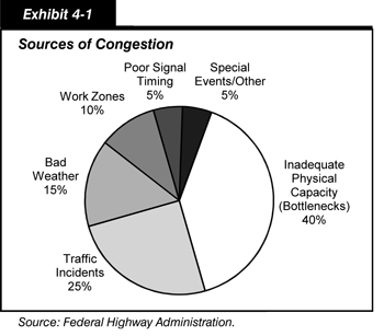
On the supply side, congestion is primarily a function of the physical characteristics of the facility and events that limit the availability of this capacity. Congestion driven by supply-side considerations is characterized as either “recurring” or “nonrecurring.” This distinction is useful in helping transportation professionals devise strategies that will either mitigate or reduce congestion. Recurring congestion happens in roughly the same time and place on the same days of the week. It results when physical capacity is simply not adequate to accommodate demand during peak periods. On the other hand, nonrecurring congestion is caused by events such as work zone activity, traffic incidents, and bad weather. Obviously, when these nonrecurring events occur on an already congested facility, the impacts are magnified. Exhibit 4-1 shows the estimated percentages of on the road congestion caused by different factors.
Congestion Measurement
There is no universally accepted definition or measurement of exactly what constitutes a congestion “problem.” The public’s perception seems to be that congestion is getting worse, and it is by many measures. However, the perception of what constitutes a congestion problem varies from place to place. Traffic conditions that may be considered a congestion problem in a city of 300,000 may be perceived differently in a city of 3 million, based on differing congestion histories and driver expectations. These differences of opinion make it difficult to arrive at a consensus of what congestion means, the effect it has on the public, its costs, how to measure it, and how best to correct or reduce it. Because of this uncertainty, transportation professionals examine congestion from several perspectives.
Three key aspects of congestion are severity, extent, and duration. The severity of congestion refers to the magnitude of the problem or the degree of congestion experienced by drivers. The extent of congestion is defined by the geographic area or number of people affected. The duration of congestion is the length of time that the roadway is congested, often referred to as the “peak period” of traffic flow.
Texas Transportation Institute Performance Measures
The Texas Transportation Institute (TTI) has studied congestion trends since 1982. Its study results are published annually in the Urban Mobility Report, which is cited nationwide for its list of congestion delays and potential solutions in the Nation's busiest cities. The Federal Highway Administration (FHWA) coordinates with TTI to establish and refine the performance metrics of congestion that provide a better indication of congestion’s level of impact on the Nation’s communities. Since 1982, the data source for the calculations in the Urban Mobility Report has been the FHWA Highway Performance Monitoring System (HPMS).
This section draws upon data computed by TTI for the FHWA using a methodology consistent with the 2009 TTI Urban Mobility report. This analysis combines information on 458 urban communities with a total population of 213 million or slightly more than 70.7 percent of the Nation’s population in 2007.
|
Alternate Congestion Measurement Approach The CEOs for Cities report, “Driven Apart,” suggests an alternative approach to the Texas Transportation Institute’s (TTI) approach to measuring congestion. Their alternative is built on the basic premise that it would be better to have trip-based measures rather than facility-based measures (as TTI’s are), especially for supporting Livable Communities. The full “Driven Apart” report may be found at http://www.ceosforcities.org/driven-apart. |
TTI divides the communities in the Urban Mobility report into four groups based on population size. In the 2009 report, 377 urbanized areas had populations of less than 500,000 and were classified as “Small,” 35 areas had populations between 500,000 and 999,999 and were classified as “Medium,” 29 areas with populations between 1 million and 3 million were classified as “Large,” and 17 areas had populations greater than 3 million and were classified as “Very Large.” These shorthand terms have been adopted in this section for clarity. However, it should be noted that they are not consistent with the population break of 200,000 frequently used in other FHWA applications to distinguish “Small Urbanized Areas” from “Large Urbanized Areas.” (Transportation Management Areas with a population greater than 200,000 are subject to additional transportation planning requirements beyond those of smaller urbanized areas.)
As urban areas increase in size, they will migrate between the four categories used by TTI to define population groups. This adjustment due to population change can have a significant impact on the results for a particular group. TTI recalculates the measures for each group for each year of data.
Average Daily Percentage of Vehicle Miles Traveled Under Congested Conditions
The average daily percent of vehicles miles traveled (VMT) under congested conditions is defined as the percentage of daily traffic on freeways and principal arterials in urbanized areas moving at less than free-flow speeds. Based on the TTI calculations, Exhibit 4-2 shows that this measure of extent and duration of congestion increased from 27.0 percent in 2000 to 28.6 percent in 2004, before dropping to 26.3 percent in 2008. As noted in Chapter 2, total VMT declined between 2006 and 2008, making it easier for existing highway facilities to accommodate the lesser demand.
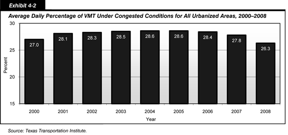
Exhibit 4-3 shows the trend of VMT under congested conditions broken down by population area size. From 2000 to 2008, the value for this measure of congestion increased for both the Small (population less than 500,000) and Medium (population 500,000 to 999,999) categories, suggesting an overall decline in operational performance in these types of urbanized areas. Over the same period, this measure of congestion decreased in Large (population 1 million to 3 million) and Very Large (population more than 3 million), suggesting some stabilization of operational performance in these urbanized areas. The percentage of VMT under congested conditions decreased from 2006 to 2008 for each of these urbanized area population categories.
| Urbanized Area Population | 2000 | 2002 | 2004 | 2006 | 2008 |
|---|---|---|---|---|---|
| Small (less than 500,000) | 13.4% | 14.4% | 15.8% | 15.9% | 13.7% |
| Medium (500,000 to 999,999) | 20.2% | 22.6% | 22.4% | 22.4% | 21.3% |
| Large (1 million to 3 million) | 27.9% | 28.7% | 29.2% | 29.6% | 27.7% |
| Very Large (more than 3 million) | 35.9% | 37.2% | 38.0% | 37.9% | 35.4% |
| All Urbanized Areas | 27.0% | 28.3% | 28.6% | 28.4% | 26.3% |
Travel Time Index
The Travel Time Index measures the additional time required to make a trip during the congested peak travel period rather than during the off-peak period in non-congested conditions, and indicates the severity and duration of congestion. The additional time required is a result of increased traffic volumes on the roadway and the additional delay caused by crashes, poor weather, special events, or other nonrecurring incidents.
Exhibit 4-4 shows changes in the national average of the Travel Time Index for all urbanized area categories evaluated by TTI. The value of 1.24 in 2008 indicates that a trip during the peak period will require 24 percent more travel time than if the same trip were made during off-peak non-congested periods. For example, a trip of 60 minutes during the off-peak time would require 74.4 minutes during the peak period when roadway usage is higher. The Travel Time Index for the Small and Medium categories in 2008 was the same as in 2000, while that for the Large and Very Large categories declined slightly over this period.
| Urbanized Area Population | 2000 | 2002 | 2004 | 2006 | 2008 |
|---|---|---|---|---|---|
| Small (less than 500,000) | 1.11 | 1.17 | 1.12 | 1.13 | 1.11 |
| Medium (500,000 to 999,999) | 1.16 | 1.17 | 1.18 | 1.18 | 1.16 |
| Large (1 million to 3 million) | 1.24 | 1.25 | 1.26 | 1.25 | 1.23 |
| Very Large (more than 3 million) | 1.36 | 1.39 | 1.39 | 1.37 | 1.35 |
| All Urbanized Areas | 1.25 | 1.27 | 1.27 | 1.26 | 1.24 |
Average Length of Congested Conditions
The average length of congested conditions, shown in Exhibit 4-5, is a measure of the duration of congestion. This is the number of hours during a 24-hour period when traffic is operating under congested conditions, combining what is commonly thought of as the “morning rush hours” and the “evening rush hours.”
| Urbanized Area Population | Hours | ||||
|---|---|---|---|---|---|
| 2000 | 2002 | 2004 | 2006 | 2008 | |
| Small (less than 500,000) | 4.2 | 4.3 | 4.6 | 4.5 | 4.2 |
| Medium (500,000 to 999,999) | 5.5 | 5.6 | 5.7 | 5.7 | 5.4 |
| Large (1 million to 3 million) | 6.5 | 6.6 | 6.6 | 6.6 | 6.4 |
| Very Large (more than 3 million) | 7.5 | 7.6 | 7.7 | 7.6 | 7.5 |
| All Urbanized Areas | 6.2 | 6.4 | 6.4 | 6.4 | 6.2 |
The average urbanized area experienced 6.2 hours of congestion per 24-hour period in 2008, approximately the same as in 2000. Over this period, Medium and Large urbanized areas experienced slight decreases in their average daily length of congestion.
In the past, recurring congestion tended to occur only in one direction—toward downtown in the morning and away from it in the evening. Today, two-directional congestion is common, particularly on routes serving several major activity centers dispersed in suburban areas around the most congested metropolitan areas.
Cost of Congestion From TTI Urban Mobility Report
Congestion has an adverse impact on the American economy, which values speed, reliability, and efficiency. The problem is of particular concern to firms involved in logistics and distribution. As just-in-time delivery increases, firms need an integrated transportation network that allows for the reliable, predictable shipment of goods. If travel time increases or reliability decreases, businesses will need to increase average inventory levels to compensate, which will increase storage costs. Congestion, then, imposes a real economic cost for businesses and these costs will continue to impact consumer prices.
As shown in Exhibit 4-6, the TTI 2009 Urban Mobility Report estimates that drivers experienced 4.2 billion hours of delay and wasted approximately 2.8 billion gallons of fuel during delays in 2007. The total congestion cost for these areas, including wasted fuel and time, was estimated to be approximately $87.2 billion. Each of these values is over four times higher than the comparable estimates for 1982, reflecting a significant increase in congestion over this 25-year period.
| Year | Total Delay (Billions of Hours) | Total Fuel Wasted (Billions of Gallons) | Total Cost (Billions of 2007 Dollars) |
|---|---|---|---|
| 1982 | 0.79 | 0.50 | $16.7 |
| 1983 | 0.87 | 0.54 | $18.0 |
| 1984 | 0.95 | 0.60 | $19.7 |
| 1985 | 1.10 | 0.70 | $22.6 |
| 1986 | 1.27 | 0.81 | $25.2 |
| 1987 | 1.41 | 0.92 | $27.9 |
| 1988 | 1.62 | 1.06 | $32.0 |
| 1989 | 1.78 | 1.17 | $35.3 |
| 1990 | 1.88 | 1.25 | $37.3 |
| 1991 | 1.90 | 1.29 | $38.1 |
| 1992 | 2.05 | 1.37 | $40.6 |
| 1993 | 2.17 | 1.43 | $42.6 |
| 1994 | 2.26 | 1.49 | $44.3 |
| 1995 | 2.42 | 1.61 | $47.8 |
| 1996 | 2.58 | 1.72 | $51.0 |
| 1997 | 2.73 | 1.82 | $53.6 |
| 1998 | 2.83 | 1.91 | $55.0 |
| 1999 | 3.04 | 2.05 | $58.9 |
| 2000 | 3.18 | 2.14 | $63.1 |
| 2001 | 3.33 | 2.25 | $65.7 |
| 2002 | 3.52 | 2.38 | $69.3 |
| 2003 | 3.73 | 2.53 | $73.3 |
| 2004 | 3.97 | 2.69 | $79.4 |
| 2005 | 4.18 | 2.82 | $85.6 |
| 2006 | 4.20 | 2.85 | $87.1 |
| 2007 | 4.16 | 2.81 | $87.2 |
Effect of Congestion on Freight Travel
FHWA’s Office of Freight Management and Operations is leading a freight performance measurement (FPM) research initiative that focuses on measuring average operating speeds and travel time reliability on freight significant corridors and on crossing time and crossing time reliability at major U.S. international land border crossings. Measures are based primarily on vehicle location and time data from communication technology used by the freight industry. Through this initiative, FHWA directly measures operating speeds and reliability on major truck routes by tracking more than 500,000 trucks. Average truck speeds drop below 55 miles per hour near major urban areas, border crossings and gateways, and in mountainous terrain.
The data produced through the FPM initiative enables FHWA to analyze freight system performance (truck speed and travel time reliability) by location, date, and time of day. As an example, Exhibit 4-7 demonstrates how the data can be used to example freight performance in peak versus nonpeak period hours, drawing upon information gathered from January through March of 2009. As would be expected, average speeds in the peak period between 6 a.m. and 9 a.m. and between 4 p.m. and 7 p.m. are lower than those recorded in the nonpeak period between 10 a.m. and 2 p.m. on all routes.
|
Freight Performance Measurement FHWA has been collecting and analyzing data for freight significant Interstate corridors since 2004. FHWA plans to continue to collect travel time information on 25 interstate corridors and 15 U.S./Canada land border crossings at least through September 2011. Key objectives of the current FPM research program are to expand on the existing data sources, further develop and refine methods for analyzing data, derive national measures of congestion and reliability, analyze freight bottlenecks and intermodal connectors and develop data products and tools that will assist DOT, FHWA, and State and local transportation agencies in addressing surface transportation congestion. A Web tool for disseminating FPM data on the 25 study corridors, www.freightperformance.org, provides an example of the types of tools FHWA will develop. The goal is to evolve the research into a credible freight data source that can be used to continuously measure freight performance and inform the development of strategies and tactics for managing and relieving freight congestion. |
| Interstate Route | Average Operating Speed | Average Speed* Peak Period | Average Speed Nonpeak Period | Interstate Route | Average Operating Speed | Average Speed Peak Period | Average Speed Nonpeak Period |
|---|---|---|---|---|---|---|---|
| 5 | 52.8 | 52.1 | 53.1 | 70 | 56.8 | 56.5 | 57.1 |
| 10 | 57.4 | 56.7 | 57.6 | 75 | 56.7 | 56.1 | 57.0 |
| 15 | 56.7 | 56.2 | 56.9 | 76 | 54.5 | 54.5 | 54.8 |
| 20 | 59.2 | 58.8 | 59.3 | 77 | 54.7 | 54.3 | 55.1 |
| 24 | 57.2 | 56.6 | 57.4 | 80 | 57.7 | 57.4 | 57.9 |
| 25 | 59.0 | 58.5 | 59.3 | 81 | 56.6 | 56.6 | 56.8 |
| 26 | 53.7 | 53.3 | 54.6 | 84 | 54.2 | 53.3 | 54.9 |
| 35 | 56.8 | 56.0 | 57.0 | 85 | 57.3 | 56.5 | 57.4 |
| 40 | 58.6 | 58.4 | 58.8 | 87 | 54.1 | 53.8 | 54.5 |
| 45 | 54.9 | 53.9 | 55.4 | 90 | 57.1 | 56.8 | 57.4 |
| 55 | 57.0 | 56.8 | 57.2 | 91 | 53.4 | 52.9 | 54.2 |
| 65 | 57.9 | 57.3 | 58.2 | 94 | 56.7 | 56.2 | 56.8 |
| 95 | 56.2 | 55.2 | 56.3 |
Emerging Operational Performance Measures
Substantial research supports the use of delay as a measure of congestion. Delay is certainly important; it exacts a substantial cost from the traveler and, consequently, from the consumer. However, it does not tell the complete story. Moreover, there currently is no direct measure of delay that can be collected both consistently and inexpensively.
Reliability is another important characteristic of any transportation system, one that industry in particular requires for efficient production. If a given trip requires 1 hour on one day and 1.5 hours on another day, an industry that is increasingly reliant on just-in-time delivery suffers. To compensate for variable trip times required to deliver products, an industry may be required to carry greater inventory than would otherwise be necessary, thereby incurring higher costs. Travel time reliability is a measure of congestion easily understood by a wide variety of audiences, and is one of the more direct measures of the effects of congestion on the highway user. However, additional research is needed to determine what measures should be used to describe congestion and what data will be required to supply these measures.
System Reliability
Travel time reliability measures are relatively new, but a few have proven useful, especially at the local level. Such measures typically compare high-delay days with average-delay days. The simplest method identifies days that exceed the 90th or 95th percentile in terms of travel times and estimates how bad delay will be on specific routes during the worst one or two travel days each month.
The Buffer Index measures the percentage of extra time travelers must add to their average peak-hour travel time to allow for congestion delays and arrive at a location on time about 95 percent of the time. The Planning Time Index represents the total travel time that is necessary to ensure on-time arrival, including both the average travel time and the additional travel time included in the Buffer Index. Generally, the Buffer Index goes up during peak periods, when congestion occurs, indicating a reliability problem.
The Planning Time Index is especially useful because it uses a numeric scale which can be directly compared to the numeric scale of the Travel Time Index presented earlier in this chapter. While data are not currently available to support these measures at the national level, data in the 2009 TTI Urban Mobility Report were collected on planning time indicators for 19 metropolitan regions. The comparison of the Travel Time Index (in average conditions) and the Planning Time Index (for an important trip) for these 19 metropolitan areas suggest that while travelers can expect a peak-period trip to take 1.14 to 1.48 times longer than a nonpeak-period trip on average; for important trips, they should plan on needing 1.43 to 2.07 times longer in order to arrive on time approximately 95 percent of the time.
The importance of reliability is underscored by a November 2004 study, Temporary Losses of Highway Capacity and Impacts on Performance: Phase 2, produced for the FHWA by the Oak Ridge National Laboratory. Temporary capacity losses due to work zones, crashes, breakdowns, adverse weather, suboptimal signal timing, toll collection facilities, and railroad crossings caused more than 3.5 billion vehicle-hours of delay on U.S. freeways and principal arterials in 1999. For journeys on regularly congested highways during peak commuting periods, temporary capacity losses added 6 hours of delay for every 1,000 miles of travel. Americans suffer 2.5 hours of delay per 1,000 miles of travel from temporary capacity loss for journeys on roads that do not experience recurring congestion.
|
FHWA Urban Congestion Report The Urban Congestion Report (UCR) is produced quarterly and characterizes emerging traffic congestion and reliability trends at the national and city level. The reports utilize archived traffic operations data gathered from State DOTs and a private traffic information company. The reports are currently using data from 23 urban areas in the Nation. The production of these reports is a cooperative effort between the Texas Transportation Institute and FHWA. The UCR data are also being used to report Travel Time Reliability in metropolitan areas for the FHWA Strategic Plan, which is available at https://www.fhwa.dot.gov/policy/fhplan.cfm#measurement. The UCR includes only those roadways that are instrumented with traffic sensors for the purposes of real-time traffic management and/or traveler information. In many cities, this typically includes the most congested parts of the freeway system. Currently, congestion information on arterial streets is not included. The congestion information presented in these reports may not be representative of the entire roadway system in any particular city. Construction may affect the roadways that are included in this report. The congestion and reliability trends are calculated by comparing the most recent 3 months this year to the same 3 months last year. Only instrumented roadways that provided data in both years are included in the UCR. Further information can be found at http://ops.fhwa.dot.gov/perf_measurement/ucr/. |
Congestion Reduction Strategies
In considering solutions to the congestion problem, it might be useful to think of the transportation system as a limited resource, for which there is an imbalance between supply and demand. Society has several options to address this situation: make more of it (add new capacity), use it more productively (operate the system at peak condition and performance), provide alternatives to highway travel, and/or create an efficient transportation market (use congestion pricing to balance supply and demand).
Making More of It: Strategic Addition of Capacity
The traditional approach to dealing with congestion is to expand the capacity of the road network. At the beginning of the Interstate era, Federal funding provided incentives to build new highways that offered significant improvements in speed, safety, and traffic-carrying capabilities. As traffic levels increased over time, many of these roads have been widened or rebuilt with higher capacity.
The demand for new highway capacity not only is increasing, but also is dynamic in nature and location. For example, locations that were rural communities in the early 1960s are now major metropolitan areas. Increases and shifts in international trade have created new trade routes and have expanded freight access requirements at seaports and major cargo hubs. The investment analyses of Part II of this report include significant discussion of the potential impact of alternative levels of system expansion on operational performance.
Many capacity expansion projects are aimed at relieving bottlenecks. Traffic bottlenecks are specific roadway locations that routinely and predictably experience congestion because traffic volumes exceed capacity during periods of heavy demand. Bottlenecks are characterized by queues upstream and freely flowing traffic downstream. They may be compared to a storm pipe that can carry only so much water—during floods the excess water just backs up behind it, much the same as traffic at bottleneck locations. However, the situation is even worse for traffic. Once the traffic flow breaks down to stop-and-go conditions, capacity is actually reduced—fewer cars can get through the bottleneck because of the extra turbulence.
The severity of congestion at a bottleneck is related to its physical design. Some facilities were originally constructed many years ago using designs that are now considered to be antiquated. Others that have been built to extremely high design specifications are simply overwhelmed by high traffic volumes. Whatever the root cause, operational conflicts can occur at lane drops (where one or more traffic lanes are lost), weaving areas (where traffic must merge across one or more lanes to access entry or exit ramps), freeway on-ramps, freeway-to-freeway interchanges, and abrupt changes in highway alignment (such as sharp curves and hills).
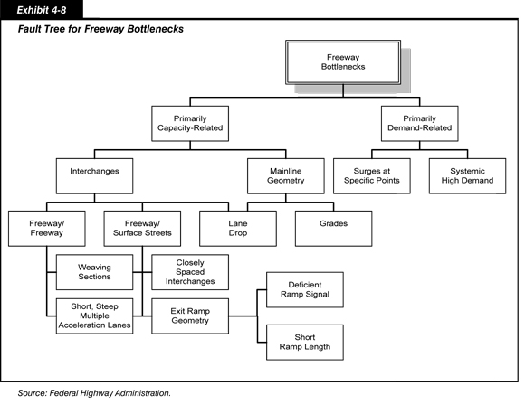
Exhibit 4-8 summarizes various root causes of freeway bottlenecks by category. Factors contributing to bottlenecks can be classified as being primarily demand-related or primarily capacity-related. Demand-related causes include both localized surges in traffic volumes at specific points and systemic high demand across an entire facility, corridor, or region. Capacity-related causes include items associated with mainline roadway geometry (grades, lane drops) and interchange design (lane drops, weaving sections, acceleration lanes, interchange spacing, ramp geometry, ramp signals, and ramp lengths). Multiple factors may contribute to causing a bottleneck at a particular location.
Bottlenecks have been the focus of transportation improvements—and of travelers’ concerns—for many years. On much of the urban highway system, there are specific points that are notorious for causing congestion on a daily basis. These locations—which can be a single interchange (usually freeway-to-freeway), a series of closely spaced interchanges, or lane drops—are focal points for congestion in corridors. Major bottlenecks tend to dominate congestion in corridors where they exist.
Some bottlenecks, particularly those involving large freeway-to-freeway interchanges, can be addressed through major construction projects. Although costly, such projects can provide congestion relief to motorists. For most other bottlenecks, however, applying operational and low-cost infrastructure solutions also may relieve congestion at much lower cost. Such strategies may include the following:
- Using a short section of shoulder as an additional travel lane during peak periods
- Restriping merge or diverge areas to better match demand
- Reducing lane widths to add a travel and/or auxiliary lane through restriping
- Modifying weaving areas (e.g., adding collector/distributor or through lanes)
- Metering or closing entrance ramps
- Adjusting speed limits when congestion thresholds are exceeded and congestion and queue formation is impending (known as speed harmonization)
- Encouraging “zippering,” the merging by alternating vehicles from two different lanes, to promote fair and smooth merges
- Designating reversible lanes to accommodate the prevailing direction of traffic flow during morning and evening peaks.
Using It More Productively: System Management and Operations
Capacity constraints arise when physical capacity is insufficient and when capacity is temporarily reduced due to traffic incidents, work zones, inclement weather, or special events. As traffic volumes have grown over time relative to physical capacity, the system has become less able to absorb “surprise”—or nonrecurring—events. In the realm of managing the highway system, the margin for error is very small and continues to decline. Operational strategies can make a major contribution to effective performance of the highway system at a much lower cost than capacity expansion because they enable quicker recovery when disruptions occur and help maximize system performance in the first place.
Such strategies include managing temporary disruptions in a way that will return the system to full capacity quickly; ensuring more effective day-to-day operations through coordinated and up-to-date traffic signal timing and operational improvements to relieve bottlenecks; and providing real-time information about the system so that travelers can decide immediately when, where, and how to travel and transportation agencies can adjust immediately to improve system operations.
| How do management and operations strategies help achieve livability and climate change goals? | |
|
As the transportation community brings livability and climate change issues into better focus, the relationship of these with management and operations strategies is becoming more apparent. Although these strategies clearly have a direct impact on reducing congestion, there currently is somewhat less of a general understanding of how they can contribute to more livable communities and reductions in greenhouse gas (GHG) emissions.
With regard to livability, management and operations strategies can help reduce congestion and delays in communities through better operation of traffic signals and more timely and effective response to traffic incidents and adverse weather conditions. Improved traffic control can enhance the safety of pedestrians and bicyclists, particularly at intersections. Traveler information strategies can provide the means for residents to make more informed mode and travel choices. And implementation of congestion pricing strategies can both reduce congestion and fund and encourage the use of alternative transportation modes. With regard to reducing GHG emissions, there are many management and operations strategies that reduce harmful emissions. These include freeway management (e.g., ramp metering), traffic incident management, road weather management, arterial management (e.g., more efficient traffic signal timing), real-time traveler information, and implementation of pricing strategies to reduce congestion. Though research on GHG reduction opportunities from management and operations strategies is limited, evaluation of individual strategies suggest the potential of a 10 percent to 20 percent reduction in GHG emissions in congested metropolitan areas if a concerted effort to implement these strategies is pursued. Livability and Sustainability are discussed in more detail in Part III of this report. |
|
Real-Time Traveler Information
Real-time traveler information enables travelers to decide how they will use (or not use) the transportation system, influencing the choices that people make about how, when, where, whether, and which way they travel to their destinations. Real-time information enables motorists to manage the uncertainty of travel during congested conditions by leaving earlier or later, taking alternative routes, or even postponing discretionary trips. Transportation agencies also can use the information to better manage and improve the system. Traveler information on traffic conditions, transit service, parking availability, and weather conditions is being delivered through various means, including Web sites, dynamic message signs, e mail and text message alerts, and highway advisory radio.
The development and establishment of 511 Traveler Information Systems to provide access to highway and travel conditions information in all parts of the Nation have been identified as key elements in implementing a successful national operations strategy. Such systems use the 511 telephone number dedicated by the Federal Communications Commission for relaying information to travelers. At the end of 2009, there were 41 active systems in 36 States, providing access to nearly 200 million people, or about 66 percent of the U.S. population.
Traffic Incident Management
As indicated in Exhibit 4-1, traffic incidents cause approximately 25 percent of all congestion; each minute of lane blockage creates 4 minutes of congestion after the incident is cleared. Traffic incident management is a planned and coordinated process to detect, respond to, and remove traffic incidents and restore capacity as safely and quickly as possible. Effectively managing traffic incidents requires cooperation among organizations that often have conflicting on-scene priorities and operating cultures. For example, transportation agencies must interact with a variety of public and private sector partners, including law enforcement, fire and rescue, emergency medical services, public safety communications, emergency management, towing and recovery, hazardous materials contractors, traffic information media, and traffic management centers (TMCs). Promoting more aggressive and widespread traffic incident management is an important strategy to lessen the effects of nonrecurring congestion as well as provide a safer driving environment.
|
Real-Time System Management Information Program Section 1201 of SAFETEA-LU requires the U.S. DOT to “establish a real-time system management information program to provide, in all States, the capability to monitor, in real time, the traffic and travel conditions of the major highways of the United States and to share that information to improve the security of the surface transportation system, to address congestion problems, to support improved response to weather events and surface transportation incidents, and to facilitate national and regional highway traveler information.” Through the Section 1201 program, agencies will be able to anticipate changes and events and take remedial actions, and provide road users with information to make better travel-related decisions. The specific goal of the program is to establish in all States the capability to share data on system performance nationwide. Significant opportunities exist for private sector involvement or partnering in implementation of this program, including information gathering, data processing, and information dissemination. Toward this end, the FHWA published an interim guidance on data-sharing specifications and data exchange formats in 2007. In May 2006, FHWA issued a notice in the Federal Register requesting comments on the proposed program goals, definitions for various parameters, the current status of related activities in the States, and implementation issues to guide development of the Real-Time System Management Information Program. In January 2009, FHWA published a notice of proposed rulemaking in the Federal Register to implement the Real-Time System Management Information Program. Based on comments received from State DOTs and other representatives of the private sector and national associations, FHWA is developing a final rule and anticipates issuing it in 2010. |
Real-time information is particularly critical for effective incident management. Information is necessary for locating and clearing crashes, stalled vehicles, spilled loads, and other highway debris. Efficient and rapid response, effective management of resources at the incident, and area-wide traffic control all depend on the rapid exchange of accurate and clear information among the responding parties. This exchange requires communications standards and institutional coordination among all the parties involved in responding to and clearing traffic incidents. (It should be noted that the term “incident delay” is sometimes used to refer to delay associated with non-recurring sources more broadly, including traffic incidents, work zones, and weather-related delays).
Work Zone Mobility
Work zones are second only to incidents as a source of delay from temporary capacity loss. Effective work zone management requires fundamental changes in the way reconstruction and maintenance projects are planned, estimated, designed, bid, and implemented. A comprehensive approach to work zone management requires minimizing work zone consequences, serving the customer around the clock, making use of real-time information, and aggressively pursuing public information and outreach.
Road Weather Management
Adverse weather is the third most common source of delay from temporary capacity loss. Although the weather cannot be changed, its effects on highway safety and operations can be reduced. Today, it is possible to predict weather changes and identify threats to the highway system with much greater precision through the use of roadside weather-monitoring equipment linked to TMCs. More precise weather information can be used to adjust speed limits and traffic signal timing; pretreat roads with anti-icing materials; pre-position trucks for deicing, sanding, or plowing; and inform travelers of changing roadway conditions.
Traffic Signal Timing and Coordination
Another source of congestion is outdated or poor signal timing at intersections. When signal timing is not updated to accommodate changes in traffic patterns, drivers may be subjected to unnecessary stops and delays. Outdated signal timing accounts for an estimated 10 percent of the total delay on major roadways, and a far greater percentage on local roadways.
Signal timing can be improved in several ways, with varying levels of complexity. At the most basic level, old signal timing plans can be updated based on more recent traffic counts. Signal controls can be upgraded, from simple signals actuated by traffic to sophisticated adaptive or even predictive computer-based controls. Interconnecting and coordinating traffic signals through a central master control can achieve the maximum benefits from traffic signal optimization.
Intelligent Transportation Systems
The range of technologies used to advance highway system operations are often referred to collectively as Intelligent Transportation Systems (ITS). They include electronic toll payment, roadway surveillance systems, and advanced traveler information systems. Such systems are being used around the country to improve the operational efficiency and safety of the transportation system. The impetus to employ ITS is growing as technology improves, congestion increases, and building new roads and bridges becomes more difficult and expensive. Many of these technologies are discussed in the highway investment analyses of Part II.
Freeway and Arterial Management Technologies. ITS technologies are being deployed to actively manage freeways and arterials in many places around the country. Ramp metering on freeways is used to regulate the flow of traffic entering a facility to increase vehicle throughput and speeds. In the Minneapolis-St. Paul region, ramp metering increased vehicle throughput by 30 percent and average speeds in the peak period by 60 percent. Adaptive signal control is another type of ITS that adjusts traffic signal timing based on real-time traffic demand. In Los Angeles, where nearly 2,500 of the more than 4,000 traffic signals use adaptive signal control, delay at intersections with these systems is reduced by an average of 10 percent.
Transportation Management Centers. A TMC coordinates the use of ITS. A TMC is typically a central location for bringing together multiple agencies, jurisdictions, and control systems for managing traffic and transit, incident and emergency response, and traveler information. Transportation management technology includes closed-circuit television cameras, dynamic message signs, synchronized traffic signals, vehicle-flow sensors, highway advisory radio, and other high-tech devices.
Active Traffic Management and Integrated Corridor Management. Active Traffic Management (ATM) is a system-centered approach to transportation management. ATM is concerned with the flow and balance within the transportation system and incorporates demand management, traffic flow management, and supply management measures. Although ATM can range from the simple to the complex, proactive management of both demand and supply greatly enhances the ability of transportation agencies to maximize the use of available highway resources including parallel routes, off-peak lanes, high-occupancy vehicle (HOV) lanes, and transit services. This approach to congestion management is a more holistic approach that can include the current U.S. application of managed lane strategies in congested freeway corridors. It is the next step in congestion management.
Integrated Corridor Management (ICM) is active traffic management at the corridor level. It focuses heavily on travel demand management and load balancing across facilities and modes. With ICM, the various institutional partner agencies manage the transportation corridor as a system. The corridor is managed as an integrated asset in order to improve travel time reliability and predictability. In an ICM corridor, because of proactive multimodal management of infrastructure assets by institutional partners, travelers can receive information that encompasses the entire transportation network. They can dynamically shift to alternative transportation options in response to changing traffic conditions.
IntelliDriveSM. In the future, vehicles communicating with other vehicles, with the roadside, and with other devices may offer significant crash prevention and congestion relief. Under the IntelliDriveSM concept being pursued by U.S. Department of Transportation (DOT), data transmitted from the roadside to the vehicle could warn a driver that it is not safe to enter an intersection. Information about traffic signal timing could be sent to vehicles to allow them to navigate arterial streets more efficiently with fewer stops. Vehicles could also serve as data collectors, anonymously transmitting traffic and road condition information from every major road. This information would allow transportation agencies to implement active strategies to relieve traffic congestion.
Providing Better Transportation Choices
In addition to managing the supply of highways, agencies may be able to affect demand for highway travel by providing attractive alternative transportation choices that meet travelers’ transportation needs at a reduced cost. The availability of less expensive travel alternatives can provide travelers with choices of location, route, time, and mode that may be more attractive than highway travel, especially under congested conditions.
Providing exclusive lanes for HOVs during peak hours is another means of providing incentives for transportation system users to reduce their use of scarce highway capacity by sharing rides in carpools, vanpools, or buses. Bike lanes and streetscape improvements can encourage the use of non-motorized travel modes. Other tools for enhancing the attractiveness and efficiency of travel alternatives include park-and-ride facilities, guaranteed ride home programs, tax-advantaged transit benefit programs, and transit-supportive local land use controls.
Other strategies are focused on shifting the times of travel or reducing the frequency and distance of trips altogether. Flexible work schedules, compressed workweeks, telecommuting, satellite work centers, and encouragement of mixed-use development (combining residential, commercial, and office uses in a single development) are among several options available to employers and public agencies in achieving such goals.
Traveler information systems are increasingly seen as an important tool for encouraging efficient travel choices by consumers. Online travel planning tools can help system users understand the likely congestion cost of travel in advance and then choose the routes and combination of modes that will most cost effectively meet their travel needs. Online tools can also be used to match carpool drivers and passengers. Real-time travel information can be used to notify travelers of traffic conditions, parking availability at remote transit stations, or even expected travel times on alternative modes.
Creating an Efficient Transportation Market: Road Pricing
Building new facilities and better management and operation of existing roads do not address one of congestion’s root causes: that most travelers do not pay the full cost of receiving transportation services. As discussed in the introduction to Part II, when making travel decisions, travelers generally consider only their own travel times and vehicle operating costs; they do not consider the effects that their trips will have on others using the same facilities. Congestion often returns to newly constructed facilities, and facilities with state-of-the-art operating practices remain congested as users respond to increases in road supply and efficiency by shifting from a less satisfactory alternatives and/or making desired trips that they might otherwise have postponed or forgone. In the absence of road pricing mechanisms, highway travel—a notably inefficient market—is distributed according to the amount of time users are willing to wait.
Congestion pricing—charging a toll during peak hours in order to bring supply and demand back into balance—relies on market forces and recognizes that trip values vary by individual, depending on time, location, destination, and cost, and more broadly among individuals, depending on personal preference and access to alternative travel options. Congestion prices can be set at levels that reflect the cost of delay that the traveler imposes on others. Travelers are encouraged to eliminate some lower value trips or take them at different times, or to choose alternate routes or modes of transportation, such as transit or carpooling.
Congestion pricing can take many forms. Presently, variable pricing is typically applied on a limited access facility (such as a bridge or highway) or in a congestion charging zone around a central business district (such as the cordon pricing zones in Stockholm, Singapore, and London). In the future, charging using global positioning systems or dedicated short-range communication technologies may make it feasible to efficiently price entire road networks.
Variable pricing can also be used to make more efficient use of existing transportation infrastructure. This provides users with the benefits of reduced congestion but at a much lower cost than adding new capacity or new technologies. For example, in Miami, Florida, as a part of the U.S. DOT Urban Partnership Program, the single HOV lane on I-95 was converted into two express lanes based on the high-occupancy toll (HOT) concept. Since the opening of the 95 Express project on December 5, 2008, the facility has serviced over 6 million vehicle trips and generated an estimated monthly toll revenue of more than $400,000. In recent surveys, 76 percent of users believe that the express lanes offer a more reliable trip than the un-tolled general purpose (GP) lanes. In addition, speeds in the GP lanes are 21 mph faster than in 2008, while the express lanes have operated at speeds in excess of 45 mph 95.4 percent of the time during the p.m. peak hours and 55.5 percent at all other times.
The 95 Express project also enhanced and expanded the Bus Rapid Transit (BRT) service on I-95 from I-395 in downtown Miami to Broward Boulevard in Fort Lauderdale. Eligibility requirements to travel toll-free in the 95 Express lanes were changed from unregistered two or more persons per vehicle (2+) to registered carpools and vanpools of three or more persons (3+) and registered hybrid vehicles. Motorcycles and emergency vehicles are permitted to use the lanes for free without registering, as are public transit vehicles, school buses, and other over-the-road coaches. Unregistered vehicles participating in the SunPass prepaid toll program are permitted to travel on 95 Express lanes for a fee in order to ensure a high probability of operating speeds of 45 mph or greater.
Congestion pricing strategies such as this retain the incentive for carpool and transit use while also reducing traffic levels in the general purpose lanes. Congestion pricing concepts can also be applied to parking. When parking is made available too cheaply, it can encourage inefficiently high levels of auto use. Underpriced parking can also contribute to localized congestion during high demand periods as motorists search for available parking spaces. Variable pricing of parking can address both of these contributors to congestion.
Transit Operational Performance
Basic goals shared by all transit operations include minimizing travel times, making efficient use of vehicle capacity, and providing reliable performance. The FTA collects data on average speed, how full the vehicles are (utilization) and how often they break down (average distance between failures) to characterize how well transit service meets these goals. These data are reported here. Though safety is also an operational issue, safety data are reported in Chapter 5, which specifically reports safety information.
More subjective customer satisfaction issues, such as how easy it is to access transit service (accessibility), and how well that service meets a community’s needs, are harder to measure. Data from the FHWA 2009 National Household Travel Survey, reported here, provide some insights but are not available on an annual basis and so does not support time series analysis. The FTA is investigating the feasibility of maintaining a database of bus stops and train stations, along with their service frequencies and other characteristics, to facilitate analysis of these issues. It is also funding research to develop measures of the degree to which transit systems contribute to the livability and sustainability of our communities. The results of this work will appear in this series of reports in future years.
New technology has allowed progressive transit agencies to report service metrics on their Web sites. Since this is a relatively new practice, measures that are standardized across the industry have not yet been developed. Industry associations are addressing this issue but for now there is no generally recognized set of standards. The FTA has proposed to perform a meta-data analysis of on-time-arrival data as posted on Web sites for major transit agencies for the next report in this series.
The following analysis presents data on average operating speeds, average number of passengers per vehicle, average percentage of seats occupied per vehicle, average distance traveled per vehicle, and mean distance between failures for vehicles. Average speed, seats occupied, and distance between failures address efficiency and customer service issues; passengers per vehicle and miles per vehicle are primarily efficiency measures. Financial efficiency metrics, including operating expenditures per revenue mile or passenger mile, are discussed in Chapter 6.
Average Operating (Passenger-Carrying) Speeds
Average vehicle operating speed is an approximate measure of the speed experienced by transit riders; it is not a measure of the operating speed of transit vehicles between stops. More specifically, average operating speed is a measure of the speed passengers experience from the time they enter a transit vehicle to the time they exit it, including dwell times at stops. It does not include the time passengers spend waiting or transferring. Average vehicle operating speed is calculated for each mode by dividing annual vehicle revenue miles by annual vehicle revenue hours for each agency in each mode, weighted by the passenger miles traveled (PMT) for each agency within the mode, as reported to the NTD. In cases where an agency contracts with a service provider, as well as provides the service directly, the speeds for each of these services within a mode are calculated and weighted separately. The results of these average speed calculations are presented in Exhibit 4-9.
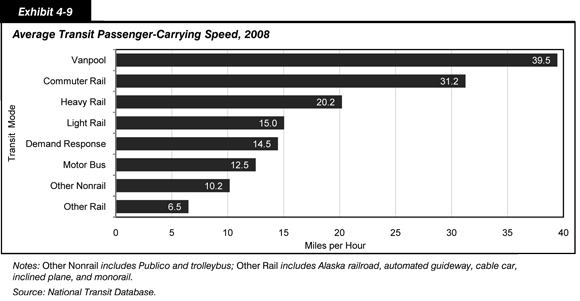
The average speed of a transit mode is strongly affected by the number of stops it makes. Motor bus service, which typically makes frequent stops, has a relatively low average speed. In contrast, commuter rail has high sustained speeds between infrequent stops, and thus a relatively high average speed. Vanpools also travel at high speeds, usually with only a few stops at each end of the route. Modes using exclusive guideway can offer more rapid travel time than similar modes that do not. Heavy rail, which travels exclusively on dedicated guideway, has a higher average speed than light rail, which often shares its guideway with mixed traffic.
Exhibit 4-10 provides average speed data for each year from 2000 to 2008 for all rail modes, all nonrail modes, and all modes combined. These average speeds are based on the average speed of each agency-mode weighted by the amount of PMT on that agency-mode. Decreases in average speed can be due to more crowded conditions—which cause longer dwell times because vehicles take on and discharge larger numbers of passengers—or to roadway congestion (bus) or track maintenance issues (rail). Average speeds for nonrail service (dominated by the bus mode) are virtually constant over the last several years. Rail service shows a slight decrease in average speed which could be due to crowding, maintenance issues, or both.
| Year | Average Speed, Miles per Hour | ||
|---|---|---|---|
| Rail | Nonrail | All Modes | |
| 2000 | 24.9 | 13.7 | 19.6 |
| 2001 | 25.2 | 13.7 | 19.6 |
| 2002 | 25.3 | 13.7 | 19.6 |
| 2003 | 25.4 | 13.9 | 20.1 |
| 2004 | 25.0 | 14.0 | 20.1 |
| 2005 | 24.0 | 13.5 | 19.2 |
| 2006 | 24.0 | 13.6 | 19.3 |
| 2007 | 24.1 | 13.5 | 19.6 |
| 2008 | 23.9 | 13.7 | 19.5 |
Vehicle Use
Vehicle Occupancy
Exhibit 4-11 shows vehicle occupancy by mode for selected years from 2000 to 2008. Vehicle occupancy is calculated by dividing PMT by vehicle revenue miles (VRMs) resulting in the average number of people carried in a transit vehicle. Aside from a possibly significant increase in heavy rail occupancy in 2008, these numbers do not indicate a meaningful increasing or decreasing trend.
| Mode | 2000 | 2002 | 2004 | 2006 | 2008 | |
|---|---|---|---|---|---|---|
| Rail | ||||||
| Heavy Rail | 23.9 | 22.6 | 23.0 | 23.2 | 25.7 | |
| Commuter Rail | 37.9 | 36.7 | 36.1 | 36.1 | 35.7 | |
| Light Rail | 26.1 | 23.9 | 23.7 | 25.5 | 24.1 | |
| Other Rail1 | 8.4 | 8.4 | 10.4 | 8.4 | 9.3 | |
| Nonrail | ||||||
| Motor Bus | 10.7 | 10.5 | 10.0 | 10.8 | 10.8 | |
| Demand Response | 1.3 | 1.2 | 1.3 | 1.3 | 1.2 | |
| Ferryboat | 120.1 | 112.1 | 119.5 | 130.7 | 118.1 | |
| Trolleybus | 13.8 | 14.1 | 13.3 | 13.9 | 14.3 | |
| Vanpool | 6.6 | 6.4 | 5.9 | 6.3 | 6.3 | |
| Other Nonrail2 | 7.3 | 7.9 | 5.8 | 7.8 | 8.2 | |
2 Aerial tramway and Público.
With vehicle capacities varying by mode, Exhibit 4-12 shows the 2008 vehicle occupancy as a percentage of the seating capacity for an average vehicle in each mode (based on the average number of seats reported per vehicle in 2008: vanpool, 11; heavy rail, 53; light rail, 63; trolleybus, 47; ferryboat, 405; commuter rail, 126; motor bus, 39; demand response, 10). For example, as shown in Exhibit 4-11, the average occupancy for a bus in 2008 was 10.8 riders and the average full-size bus seats 39 people. This occupancy, as a percentage of seating capacity, is 27.8 percent. Some modes also have substantial standing capacity that is not considered here, but which can allow the “percentage of seats occupied” measure to exceed 100 percent for a full vehicle.
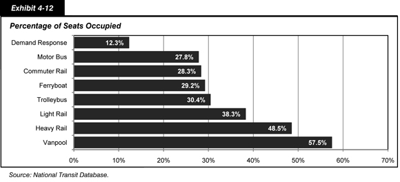
Although, on the average, it appears that there is considerable excess capacity in all these modes, it should be noted that commuting patterns make it difficult to fill vehicles returning to the suburbs from downtown employment centers during the morning rush hours and, likewise, to fill vehicles going downtown in the evening rush. Vehicles also tend to be relatively empty at the beginning and ends of their routes. For many commuter routes, a vehicle that is crush-loaded (e.g., filled to maximum capacity) on part of the trip may still only achieve an average occupancy of around 25 percent.
Revenue Miles per Active Vehicle (Service Use)
Vehicle service use, the average distance traveled per vehicle in service, can be measured by VRMs per vehicle in active service. Exhibit 4-13 provides vehicle service use by mode for selected years from 2000 to 2008. Heavy rail, generally offering long hours of frequent service, had the highest vehicle use during this period and displays a clear trend of gradually increasing service use per vehicle. Vehicle service use for light rail also appears to show an increasing trend. Vehicle service use for nonrail modes appears to be stable over the past few years with no apparent trends in either direction.
| Mode | Thousands of Revenue Vehicle Miles | Average Annual Rate of Change | ||||
|---|---|---|---|---|---|---|
| 2000 | 2002 | 2004 | 2006 | 2008 | 2008/2000 | |
| Rail | ||||||
| Heavy Rail | 55.6 | 55.1 | 57.0 | 57.2 | 57.7 | 0.5% |
| Commuter Rail | 42.1 | 43.9 | 41.1 | 43.0 | 45.5 | 1.0% |
| Light Rail | 32.5 | 41.1 | 39.9 | 39.9 | 44.1 | 3.9% |
| Nonrail | ||||||
| Motor Bus | 28.0 | 29.9 | 30.2 | 30.2 | 30.3 | 1.0% |
| Demand Response | 17.9 | 21.1 | 20.1 | 21.7 | 21.3 | 2.2% |
| Ferryboat | 24.1 | 24.4 | 24.9 | 24.8 | 21.9 | -1.2% |
| Vanpool | 12.9 | 13.6 | 14.1 | 13.7 | 14.3 | 1.3% |
| Trolleybus | 18.9 | 20.3 | 21.1 | 19.1 | 18.7 | -0.1% |
Frequency and Reliability of Service
The frequency of transit service varies considerably according to location and time of day. Transit service is more frequent in urban areas and during rush hours—namely, where and when the demand for transit is highest. Studies have found that transit passengers consider the time spent waiting for a transit vehicle to be less well spent than the time spent traveling in a transit vehicle. The higher the degree of uncertainty in waiting times, the less attractive transit becomes as a means of transportation and the fewer users transit will attract. Further, when scheduled service is offered less frequently, reliability becomes more important to users.
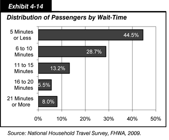
Exhibit 4-14 shows findings on wait-times from the 2009 National Household Travel Survey (NHTS) by the FHWA, the most recent nationwide survey of this information. The NHTS found that 44.5 percent of all passengers who ride transit wait 5 minutes or less and 73.2 percent wait 10 minutes or less. The NHTS also found that 8.0 percent of all passengers wait more than 20 minutes. A number of factors influence passenger wait-times, including the frequency of service, the reliability of service, and passengers’ awareness of timetables. These factors are also interrelated. For example, passengers may intentionally arrive earlier for service that is infrequent, compared with equally reliable services that are more frequent. Overall, waiting times of 5 minutes or less are clearly associated with good service that is either frequent, reliably provided according to a schedule, or both. Waiting times of 5 to 10 minutes are most likely consistent with adequate levels of service that are both reasonably frequent and generally reliable. Waiting times of 20 minutes or more indicate that service is likely both infrequent and unreliable.
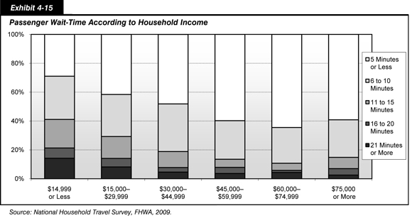
Waiting time is also correlated with income, as shown in Exhibit 4-15. Passengers from households with annual incomes of $30,000 or more are much more likely to report a waiting time of 5 minutes or less than passengers from households with incomes of less than $30,000. Additionally, passengers from households with more than $45,000 in annual income report almost never waiting more than 15 minutes for transit. This disparity is in large part due to the fact that high income riders tend to be “choice” riders who primarily ride transit on modes, routes, and at times of day when the service is frequent and reliable—and who generally substitute the use of personal automobiles for trips when these conditions aren’t met. In contrast, passengers with lower incomes are more likely to use transit for basic mobility and have more limited alternative means of travel, therefore using transit even when the service is not as frequent or reliable as they may prefer.
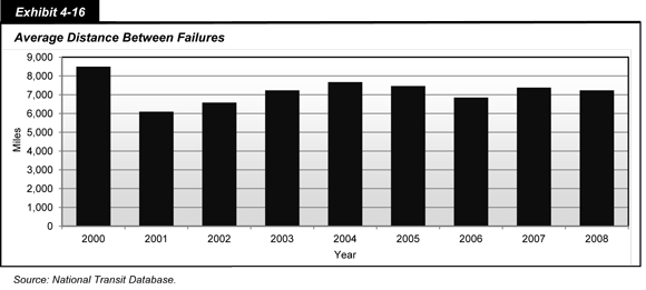
Average distance between failures, as shown in Exhibit 4-16, has been relatively stable since 2003 at around 7,000 miles. This indicates that the number of unscheduled delays due to mechanical failure of transit vehicles has not increased. The FTA does not collect data on delays due to guideway conditions; this would include congestion for roads and slow zones (due to system or rail problems) for track. These delays are not considered to be as much of a problem as delays caused by vehicle failure. This is an issue that the FTA will be addressing as part of its State of Good Repair work in the future.