

- Selected Highway Capital Investment Scenarios
- Selected Transit Capital Investment Scenarios
Selected Highway Capital Investment Scenarios
This section presents future investment scenarios that build on the Chapter 7 analyses of alternative levels of future investment in highways and bridges. Each scenario includes projections for system conditions and performance based on simulations with the Highway Economic Requirements System (HERS) and National Bridge Investment Analysis System (NBIAS). To put the modeling results in perspective, each scenario scales up the total amount of simulated investment using ratio factors to add in the types of highway and bridge investment that are beyond these models’ scopes. A subsequent section of this chapter explores transit investment scenarios that, like those of this section, start with a 2010 base year and cover the 20-year period through 2030. All the scenarios are intended to be illustrative; none of them is endorsed as a target level of funding.
Chapter 9 includes supplemental analyses relating to these scenarios, including comparisons with the investment levels presented for comparable scenarios in previous C&P reports. Chapter 10 includes a series of sensitivity analyses that explore the implications of alternative technical assumptions for the scenario investment levels. The Introduction to Part II provides critical background information relating to the technical limitations of the analysis, which are discussed further in the appendices.
Pursuant to Moving Ahead for Progress in the 21st Century (MAP-21), the National Highway System (NHS) will be expanded to include additional principal arterial and connector mileage that was not part of the original system. In light of this change, projecting future NHS investment needs over 20 years based on the system as it existed in 2010 would have limited value. Rather than dropping the NHS scenarios from the C&P report series until a formal NHS re-designation is completed, this report includes projections based on an estimate of what the system would ultimately look like by adding in principal arterials that are not currently part of the NHS. After the revised NHS designations have been coded into the HPMS and National Bridge Inventory (NBI), future editions of this report will use them for the NHS-based scenarios.
Scenarios Selected for Analysis
For the entire road network and then separately for Federal-aid highways, the NHS, and the Interstate Highway System, this section examines the four scenarios described in Exhibit 8-1. Each of these scenarios is based on capital investment by all levels of government combined. The question of what portion should be funded by the Federal government, State governments, local governments, or the private sector is beyond the scope of this report. Each scenario pairs an assumed level of total investment in the types of improvements modeled by HERS with an assumed level of investment in the types of improvements modeled by NBIAS; these levels are drawn from those considered in Chapter 7. Together, the scopes of these models cover spending on highway expansion and pavement improvements on Federal-aid highways (HERS) and on bridge rehabilitation on all highways (NBIAS). In the absence of data required for the non-modeled types of highway and bridge investment, each scenario simply assumes that their share of highway and bridge investment will remain at the 2010 percentage. Percent shares in 2010 also served to distribute the amount of non-modeled investment among the component categories: pavement spending on non-Federal-aid highways, system expansion spending on non-Federal-aid highways, and system enhancement spending (which include safety enhancements, operational improvements, and environmental projects).
| Scenario Component | Sustain 2010 Spending* | Maintain Conditions and Performance | Intermediate Improvement | Improve Conditions and Performance |
|---|---|---|---|---|
| HERS-Derived | Sustain spending on types of capital improvements modeled in HERS at 2010 levels in constant dollar terms over next 20 years | Set spending at the average of (1) the level at which projected average IRI in 2030 matches that in 2010, and (2) the level at which projected average delay per VMT in 2030 matches that in 2010 | Set spending at the level sufficient to fund all potential projects with a BCR greater than or equal to 1.5 | Set spending at the level sufficient to fund all cost-beneficial potential projects (i.e., those with a BCR greater than or equal to 1.0) |
| NBIAS-Derived | Sustain spending on types of capital improvements modeled in NBIAS at 2010 levels in constant dollar terms over the next 20 years | Set spending at the level at which the projected average bridge sufficiency rating in 2030 matches that in 2010 | Set spending at the level which achieves one-half of the projected increase to the average bridge sufficiency rating under the Improve Conditions and Performance scenario | Set spending at the level sufficient to fund all cost-beneficial potential projects |
| Other (Non-Modeled) | Sustain spending on types of capital improvements not modeled in HERS or NBIAS at 2010 levels in constant dollar terms over the next 20 years | Set spending at the level necessary so that the nonmodeled share of total highway and bridge investment will remain the same as in 2010 | Set spending at the level necessary so that the nonmodeled share of total highway and bridge investment will remain the same as in 2010 | Set spending at the level necessary so that the nonmodeled share of total highway and bridge investment will remain the same as in 2010 |
| How do the definitions of the selected scenarios presented in this report compare to those presented in the 2010 C&P Report? | |
|
The Sustain 2010 Spending scenario is defined in a manner consistent with the Sustain Current Spending scenario presented in previous editions of the C&P report; however, the scenario name was changed to emphasize that 2010 was an atypical year, since spending was boosted by one-time funding under the Recovery Act. The names and definitions of the Improve Conditions and Performance scenario and the State of Good Repair benchmark are unchanged.
The definition of the HERS-derived component of the Intermediate Improvement scenario remains unchanged. For the 2010 C&P Report, the NBIAS-derived component was defined around the average annual spending growth rate taken from the HERS-derived component; for this edition, the NBIAS-derived component has been redefined to be independent of HERS, and instead represents a level of investment that achieves half of the improvement in the average bridge sufficiency rating computed for the Improve Conditions and Performance scenario. The Maintain Conditions and Performance scenario is similar in concept to the comparable scenario in the 2010 C&P Report, in that it attempts to maintain selected performance measures at their base-year levels through the end of the 20-year analysis period; however, the target measures have been modified. The NBIAS-derived component of the scenario targets the average bridge sufficiency rating rather than the bridge investment backlog, a measure that was utilized for the last several editions of the C&P report. The HERS-derived component of the Maintain Conditions and Performance scenario had been defined around maintaining average highway user cost for several editions through the 2008 C&P Report. For technical reasons, it had become increasingly cumbersome to apply and explain this target measure, so in the 2010 C&P Report, average speed was adopted instead, in large part because it yielded similar results at the systemwide level (though this was not consistently true for subsets of the system). The HERS-derived component of this scenario used for the current edition is defined as the average of the investment level estimated to be sufficient to maintain average IRI, and the investment level estimated to be sufficient to maintain average delay. In practice, this approach results in one of these target measures improving somewhat over 20 years, while the other gets somewhat worse—an outcome consistent with the results obtained when the target measure was average highway user cost. At the systemwide level, and assuming that VMT growth conforms to HPMS forecasts, using average speed as the target measure as in the 2010 C&P Report would have produced annual average investment levels of $88.4 billion, or 2.5 percent more than what is shown in Exhibit 8-2. |
|
The projections for conditions and performance in each scenario represent estimates of what could be achieved with a given level of investment assuming an economically driven approach to project selection. They do not represent what would be achieved given current decision making practices. Consequently, comparing the relative conditions and performance outcomes across the different scenarios may be more illuminating than focusing on the specific projections for each individual scenario.
Scenario Spending Levels
Future spending levels by scenario, summarized in Exhibit 8-2, are stated in constant 2010 dollars. (Chapter 9 illustrates how to convert these real-dollar values into nominal [future dollar] values that factor in inflation beyond 2010.) The modeling on which the scenarios are based (which was presented in Chapter 7) assumes that spending grows at an annual percent rate that does not vary over the 20-year analysis period, but which differs between the types of investments modeled by HERS and those modeled by NBIAS, and also in some scenarios according to the assumed rate of future traffic growth. (The average annual investment levels are determined by summing the amounts expended for each year from 2011 through 2030 under the scenario, and dividing by 20.)
The application of the four illustrative scenarios to different highway systems produces the subscenarios in Exhibit 8-2. For example, the subscenario for Federal-aid highways in the Sustain 2010 Spending scenario fixes average annual spending on those highways at what was actually spent in 2010, $75.8 billion, without likewise forcing the portions of that spending directed to the NHS or the Interstate System to match their 2010 levels. Differences between these portions and the corresponding base-year amounts arise because HERS and NBIAS rely on benefit-cost principles to flexibly allocate spending among potential improvements within their scope.
For each of the other scenarios in Exhibit 8-2, the spending levels vary according to the future growth rate assumed for vehicle miles traveled (VMT). As discussed in Chapter 7, the VMT forecasts from the HPMS imply an average annual growth rate of 1.85 percent, whereas the 15-year trend growth (between 1995 and 2010) was only 1.36 percent. Assuming that future growth follows the trend rather than the forecast rate reduces the spending level associated with achieving scenario goals related to pavement improvements and system expansion, which are modeled with HERS. The needs for bridge rehabilitation spending are less sensitive to changes in VMT growth, so the implied traffic growth from the NBI forecasts was used to generate all of the NBIAS inputs to these scenarios.
The Maintain Conditions and Performance scenario is geared toward maintaining overall conditions and performance on the particular portion of the road network to which the scenario is being applied. For example, when the scenario relates to maintaining average conditions and performance on Federal-aid highways, it may entail improvement or deterioration in average conditions and performance on subsets of these highways, such as the Interstate Highway System. The models used to simulate the scenarios, HERS and NBIAS, are each designed to determine the investment program that will minimize the cost of achieving the scenario goal.
Spending Levels Assuming Forecast Growth in VMT
The Maintain Conditions and Performance scenario uses average pavement roughness, average delay per VMT, and average bridge sufficiency rating as the measures of overall system conditions and performance that it seeks to maintain. Although the system to which these goals pertain varies across the subscenarios, the average annual amount of investment is uniformly less than actual 2010 spending. A major reason for this pattern is that the 2010 level of investment was quite high by historical standards (due largely to the Recovery Act), particularly for system rehabilitation spending. (For a discussion of highway and bridge investment trends, see Chapter 6). Highway capital spending increased by 10.8 percent between 2008 and 2010 in nominal dollar terms while highway construction costs dropped by 18.0 percent. Factoring in this price change, capital spending grew by 35.1 percent in constant dollar terms between 2008 and 2010.
| Scenario and Comparison Parameter | Assuming Higher VMT Growth Derived from HPMS Forecasts1 | Assuming Lower, Trend-Based VMT Growth2 | ||||
|---|---|---|---|---|---|---|
| Interstate System | NHS3 | Federal-Aid Highways | All Roads | Federal-Aid Highways | All Roads | |
| Sustain 2010 Spending Scenario4 | ||||||
| Average Annual Investment (Billions of 2010 Dollars), for 2011 through 2030 | $20.2 | $53.9 | $75.8 | $100.2 | $75.8 | $100.2 |
| Maintain Conditions and Performance Scenario | ||||||
| Average Annual Investment (Billions of 2010 Dollars), for 2011 Through 2030 | $17.4 | $37.8 | $67.3 | $86.3 | $50.3 | $65.3 |
| Percent Difference Relative to 2010 Spending4 | -14.1% | -29.8% | -11.2% | -13.9% | -33.6% | -34.8% |
| Annual Spending Increase Needed to Support Scenario Investment Level5 | -1.47% | -3.51% | -1.15% | -1.44% | -4.08% | -4.29% |
| Intermediate Improvement Scenario | ||||||
| Average Annual Investment (Billions of 2010 Dollars), for 2011 Through 2030 | $27.8 | $58.8 | $87.6 | $111.9 | $73.1 | $93.9 |
| Percent Difference Relative to 2010 Spending4 | 37.8% | 9.2% | 15.6% | 11.7% | -3.5% | -6.3% |
| Annual Spending Increase Needed to Support Scenario Investment Level5 | 2.96% | 0.83% | 1.36% | 1.04% | -0.34% | -0.62% |
| Improve Conditions and Performance Scenario | ||||||
| Average Annual Investment (Billions of 2010 Dollars), for 2011 through 2030 | $33.1 | $74.9 | $113.7 | $145.9 | $95.7 | $123.7 |
| Percent Difference Relative to 2010 Spending4 | 64.0% | 39.1% | 50.1% | 45.7% | 26.4% | 23.4% |
| Annual Spending Increase Needed to Support Scenario Investment Level5 | 4.51% | 3.05% | 3.72% | 3.46% | 2.18% | 1.96% |
| State of Good Repair Benchmark6 | ||||||
| Average Annual Investment (Billions of 2010 Dollars), for 2011 Through 2030 | $13.2 | $34.5 | $60.4 | $78.3 | $57.2 | $72.9 |
2 As discussed in Chapter 7, the average annual growth rate for the 15-year period from 1995 to 2010 was 1.36 percent, and is referenced as the "Trend" VMT growth. HERS assumes this represents the VMT that would occur at a constant price, and adjusts the growth rate for the individual scenarios in response to changes in highway user costs. NBIAS is less sensitive to changes in VMT growth, and the implied traffic growth from the NBI was used to generate all of the NBIAS inputs to these scenarios.
3 The NHS statistics presented in this chapter are intended to approximate the NHS as it will exist after its expansion directed by MAP-21, not the NHS as it existed in 2010.
4 Highway capital spending in 2010 was boosted by one-time funding under the Recovery Act.
5 This percentage represents the annual percent change for each year relative to 2010 that would be required to achieve the average annual funding level specified for the scenario in constant dollar terms. Additional increases in nominal dollar terms would be needed to offset the impact of future inflation. Negative values indicate that the average annual investment level associated with the scenario is lower than 2010 spending.
6 The State of Good Repair benchmark is the subset of the Improve Conditions and Performance scenario that pertains to system rehabilitation investments only, and excludes investments in system expansion and system enhancement.
For the version of the Maintain Conditions and Performance scenario focused on all roads (and assuming HPMS forecast VMT growth), the average annual investment level of $86.3 billion is 13.9 percent lower than actual 2010 capital spending of $100.2 billion on all roads; the goals of this subscenario could be achieved even if capital spending declined by 1.44 percent per year over 20 years in constant dollar terms. Similar percentage differences are evident in the subscenarios for Federal-aid highways (11.2 percent) and Interstate highways (14.1 percent). The outlier is the sub-scenario for the NHS, where the level of investment to maintain conditions and performance is estimated to be 29.8 percent lower than the amount of investment directed to that system in 2010. Because the Interstate highways form a significant portion of the NHS, this implies relatively sharp reductions in spending for the remaining portion off of the Interstate System. Annual percentage growth rates in spending are between -1.0 percent and -1.5 percent across subscenarios, except for the -3.5 percent annual decline in spending indicated to be consistent with maintaining overall conditions and performance on the NHS. It is important to note that because 2010 highway capital spending included one-time funding under the Recovery Act, sustaining this level of investment in the future would present a greater challenge than would be the case for a more typical base year.
Unless one is completely satisfied with base year conditions and performance, investing at a level projected to maintain that level of performance would not yield an ideal result. The analyses reflected in the Improve Conditions and Performance scenario suggest that an economically driven approach to investment that funds all cost-beneficial improvements would substantially increase real spending on highways and bridges above base-year levels. Assuming forecast VMT growth for the 2011–2030 analysis period, the annual percent increase in investment associated with implementation of all cost-beneficial capital improvements is 4.51 percent for the Interstate highways, 3.05 percent for the NHS, 3.72 percent for Federal-aid highways, and 3.46 percent for all roads. The associated levels of average annual spending represent an investment ceiling above which it would not be cost-beneficial to invest even if available funding were unlimited, and exceed the 2010 levels by 64.0 percent for Interstate highways, 39.1 percent for the NHS, 50.1 percent for Federal-aid highways, and 45.7 percent for all roads. For all roads, the average annual spending amounts to fully implement all cost-beneficial investments is estimated to be $145.9 billion, or $2.9 trillion over the 20-year period, stated in constant 2010 dollars.
The State of Good Repair benchmark represents the portion of average annual spending that the Improve Conditions and Performance scenario allocates to system rehabilitation investments. Put at $78.3 billion in Exhibit 8-2 for all roads, this benchmark represents the amount of cost-beneficial investment identified for rehabilitation of existing pavements and bridges. In determining the size of this benchmark, HERS and NBIAS screen out through benefit-cost analysis any assets that may have outlived their original purpose, rather than automatically re-investing in all assets in perpetuity. With national consensus lacking on exactly what constitutes a “state of good repair” for the various transportation assets, alternative benchmarks with different objectives could be equally valid from a technical perspective.
| Does the State of Good Repair benchmark apply the same criteria for all types of roadways modeled in HERS? | |
|
No. For principal arterials, the deficiency levels in HERS have been set so that the model will consider taking action on a pavement only when its International Roughness Index (IRI) value has risen above 95 (inches per mile), meaning that it would no longer be considered to have “good” ride quality based on the criteria described in Chapter 3.
For roads functionally classified as collectors, the HERS deficiency levels have been set so that pavement actions will only be considered when IRI values have risen above 170, and the roads, thus, no longer meet the criteria for “acceptable” ride quality. The IRI threshold for minor arterials is set at 120. Although the engineering thresholds identified above define when the model may consider a pavement improvement, any such improvement must pass a benefit-cost test in order to be implemented. Even when HERS is given an unlimited budget to work with, it does not recommend improving all principal arterials to the “good” ride quality level, or all collectors to the “acceptable” ride quality level. The specific IRI value at which a pavement improvement will pass a benefit-cost test depends on a number of factors, including the traffic volume and average speeds on that facility. As discussed in Chapter 3, pavement ride quality has a greater impact on highway user costs on higher-speed roads. |
|
The goal of the Intermediate Improvement scenario is to partially achieve the performance improvements associated with the economically driven approach to investment taken in the Improve Conditions and Performance scenario. For bridge rehabilitation spending, the Intermediate Improvement scenario seeks to achieve half of the improvement in the average bridge sufficiency rating; for spending on pavement rehabilitation and highway expansion, the scenario implements all projects with a benefit-cost ratio (BCR) of 1.5 or greater, as opposed to 1.0 or greater in the Improve Conditions and Performance scenario. (Applying a minimum BCR cutoff higher than 1.0 reduces the risk of investing in projects that initially appear cost beneficial but do not prove so due to unexpected changes in future costs or travel demand.) Assuming forecast VMT growth for 2011–2030, the average annual spending in the Intermediate Improvement scenario for all roads, $111.9 billion, exceeds the actual 2010 level by $11.7 billion, which is about one-fourth of the $45.7 billion increase indicated in the Improve Conditions and Performance scenario. For the Federal-aid highways and the NHS, the corresponding proportion is similar to that for all roads, but, for the Interstate System, the increase in spending relative to 2010 under the Intermediate Improvement scenario amounts to nearly three-fifths of the increase under the Improve Conditions and Performance scenario.
Spending Levels Assuming Trend Growth in VMT
Replacing the overall rate of traffic growth implied by the HPMS forecasts with the 15-year historic trend rate of growth reduces the scenario levels of spending substantially. Annual spending in the Maintain Conditions and Performance scenario averages $65.3 billion for all roads and $50.3 billion for Federal-aid highways, which are each about 25 percent lower than when the overall rate of VMT growth from the HMPS forecasts was used. For the Intermediate Improvement and Improve Conditions and Performance scenarios, the spending reductions from the forecast growth case are smaller, at about 16 percent. The results for annual percent growth in spending show spending decreasing at just over 4 percent per year in the Maintain Conditions and Performance scenario, and at less than one percent in the Intermediate Improvement scenario. Only in the Improve Conditions and Performance scenario does spending increase, at about 2 percent per year, when trend growth in traffic is assumed.
Scenario Spending Patterns and Conditions and Performance Projections
The following discussion details the derivation of scenario spending levels, the patterns in spending by type of improvement and highway functional class, and the projections for conditions and performance.
Systemwide Scenarios
For the scenarios that consider all roads, the derivation of the average annual investment levels is presented in Exhibit 8-3 (forecast-based VMT growth) and Exhibit 8-4 (trend-based VMT growth). The HERS-derived component, which accounts in each scenario for most of the total investment, represents spending on pavement rehabilitation and capacity expansion on Federal-aid highways. The NBIAS-derived component represents rehabilitation spending on all bridges, including those not on the Federal-aid highways. In the Sustain 2010 Spending scenario, the values for these components sum to $72.5 billion, of which $56.4 billion is the HERS-derived component. Nonmodeled spending accounted in 2010 for 26.6 percent of total investment ($26.7 billion out of $100.2 billion) and is assumed to form the same share in all scenarios. The non-modeled spending is allocated among types of capital improvements according to its 2010 percent distribution: 36.7 percent, system rehabilitation (non-Federal-aid highways); 15.4 percent, system expansion (non-Federal-aid highways), and 47.9 percent, system enhancements. Because they include non-modeled spending, the amounts shown in any scenario for the “system rehabilitation-highway” and “system expansion” categories sum to more than the HERS-derived component of spending.
| Sustain 2010 Spending Scenario | Maintain Conditions & Performance Scenario | Intermediate Improvement Scenario | Improve Conditions & Performance Scenario | |
|---|---|---|---|---|
| Scenario Derivation, by Input Components* | ||||
| Average Annual Investment (Billions of 2010 Dollars) | $100.2 | $86.3 | $111.9 | $145.9 |
| HERS-Derived Component (Billions of 2010 Dollars) | $56.4 | $51.1 | $67.8 | $86.9 |
| Percent of Scenario Derived from HERS | 56.3% | 59.2% | 60.6% | 59.5% |
| Annual Percent Change in HERS Spending | 0.0% | -1.0% | 1.7% | 4.0% |
| Minimum BCR for HERS-Derived Component | 1.92 | 2.17 | 1.50 | 1.00 |
| NBIAS-Derived Component (Billions of 2010 Dollars) | $17.1 | $12.2 | $14.3 | $20.2 |
| Percent of Scenario Derived from NBIAS | 17.0% | 14.1% | 12.8% | 13.8% |
| Annual Percent in NBIAS Spending | 0.0% | -3.3% | -1.7% | 1.6% |
| Other Component (Billions of 2010 Dollars) | $26.7 | $23.0 | $29.8 | $38.8 |
| Percent of Scenario Derived from Other | 26.6% | 26.6% | 26.6% | 26.6% |
| Distribution by Capital Improvement Type, Average Annual (Billions of 2010 Dollars) | ||||
| System Rehabilitation-Highway | $40.4 | $36.5 | $46.5 | $58.1 |
| System Rehabilitation-Bridge | $17.1 | $12.2 | $14.3 | $20.2 |
| System Rehabilitation-Total | $57.4 | $48.7 | $60.8 | $78.3 |
| System Expansion | $30.0 | $26.6 | $36.8 | $49.0 |
| System Enhancement | $12.8 | $11.0 | $14.3 | $18.6 |
| Total, All Improvement Types | $100.2 | $86.3 | $111.9 | $145.9 |
| Percent Distribution by Capital Improvement Type | ||||
| System Rehabilitation | 57.3% | 56.5% | 54.4% | 53.7% |
| System Expansion | 29.9% | 30.8% | 32.9% | 33.6% |
| System Enhancement | 12.8% | 12.8% | 12.8% | 12.8% |
The minimum BCR associated with the HERS components of the Improve Conditions and Performance scenario (1.0) and the Intermediate Improvement scenario (1.5) are the same whether forecast VMT growth or trend-based VMT growth is assumed, as these scenarios are defined around these particular BCR levels. For the Sustain 2010 Spending scenario, the minimum BCR of 1.92 assuming forecast VMT growth (Exhibit 8-3) is higher than the minimum BCR of 1.42 assuming trend-based VMT growth (Exhibit 8-4) because higher future travel volumes would tend to increase the benefits associated with both pavement and capacity improvements. For the Maintain Conditions and Performance scenario, the minimum BCR of 2.17 assuming forecast VMT growth is higher than the minimum BCR of 1.42 assuming trend-based VMT growth primarily because the average annual investment level associated with achieving the goals of this scenario is considerably higher assuming forecast VMT growth, so HERS would need to move further down its BCR-prioritized list of potential improvements.
| Sustain 2010 Spending Scenario | Maintain Conditions & Performance Scenario | Intermediate Improvement Scenario | Improve Conditions & Performance Scenario | |
|---|---|---|---|---|
| Scenario Derivation, by Input Components* | ||||
| Average Annual Investment (Billions of 2010 Dollars) | $100.2 | $65.3 | $93.9 | $123.7 |
| HERS-Derived Component (Billions of 2010 Dollars) | $56.4 | $35.7 | $54.6 | $70.5 |
| Percent of Scenario Derived from HERS | 56.3% | 54.7% | 58.1% | 57.1% |
| Annual Percent Change in HERS Spending | 0.0% | -4.6% | -0.3% | 2.1% |
| Minimum BCR for HERS-Derived Component | 1.42 | 2.53 | 1.50 | 1.00 |
| NBIAS-Derived Component (Billions of 2010 Dollars) | $17.1 | $12.2 | $14.3 | $20.2 |
| Percent of Scenario Derived from NBIAS | 17.0% | 18.7% | 15.3% | 16.3% |
| Annual Percent in NBIAS Spending | 0.0% | -3.3% | -1.7% | 1.6% |
| Other Component (Billions of 2010 Dollars) | $26.7 | $17.4 | $25.0 | $32.9 |
| Percent of Scenario Derived from Other | 26.6% | 26.6% | 26.6% | 26.6% |
| Distribution by Capital Improvement Type, Average Annual (Billions of 2010 Dollars) | ||||
| System Rehabilitation-Highway | $43.4 | $29.0 | $41.8 | $52.7 |
| System Rehabilitation-Bridge | $17.1 | $12.2 | $14.3 | $20.2 |
| System Rehabilitation-Total | $60.4 | $41.2 | $56.1 | $72.9 |
| System Expansion | $26.9 | $15.8 | $25.8 | $35.0 |
| System Enhancement | $12.8 | $8.3 | $12.0 | $15.8 |
| Total, All Improvement Types | $100.2 | $65.3 | $93.9 | $123.7 |
| Percent Distribution by Capital Improvement Type | ||||
| System Rehabilitation | 60.3% | 63.1% | 59.8% | 58.9% |
| System Expansion | 26.9% | 24.1% | 27.5% | 28.3% |
| System Enhancement | 12.8% | 12.8% | 12.8% | 12.8% |
Spending by Improvement Type
In the Improve Conditions and Performance scenario, annual spending on highway and bridge rehabilitation averages $78.3 billion assuming forecast VMT growth and $72.9 billion assuming trend VMT growth, in either case considerably more than the $60.0 billion of such spending in 2010 identified in Chapter 6. This suggests that achieving a state of good repair on the Nation’s highways would require either a significant increase in overall highway and bridge investment or a significant redirection of investment from other types of improvements toward system rehabilitation.
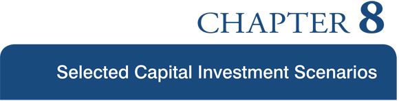
Exhibit 8-5 compares the distributions from the preceding two exhibits for investment spending by improvement type with the actual distribution of capital spending in 2010. When higher VMT growth is assumed (based on HPMS forecast), system expansion comprises between 29.9 percent and 33.6 percent of each scenario’s total investment in highways and bridges, somewhat higher than its actual 27.4 percent share of such spending in 2010. The share of spending directed to rehabilitation is correspondingly lower in each scenario than it was in 2010; the sharpest decline is indicated for bridge rehabilitation spending, which attracts only 13.1 percent of spending in the Improve Conditions and Performance scenario versus 17.0 percent in 2010.
When lower VMT growth is assumed (based on the 15-year historic trend), compared with its actual 27.4 percent share in 2010, the system expansion share of spending is virtually the same in the Intermediate Improvement scenario, 3.3 percentage points lower in the Sustain 2010 Spending scenario, and marginally higher or lower in the other scenarios. In each scenario, the system expansion share of spending assuming trend-based VMT growth is lower than where a higher VMT growth rate is assumed—in the Improve Conditions and Performance scenario, for example, 28.3 percent versus 33.6 percent. This reflects that benefits from system expansion projects tend to be more sensitive to future traffic volumes than benefits from system rehabilitation projects.
Projections for 2030 Conditions and Performance
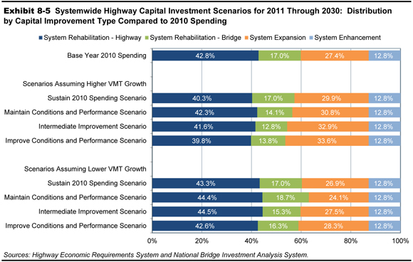
Since the HERS model considers only Federal-aid highways, whereas NBIAS considers bridges on all roads, the only conditions and performance indicators available for the systemwide scenarios are those for bridges. Exhibit 8-6 presents projections for the average bridge sufficiency index . Apart from the Maintain Conditions and Performance scenario, the values of this index projected for 2030 indicate improvement on the 2010 base year values. The largest improvement is in the Improve Conditions and Performance scenario, where spending on bridge rehabilitation is at the highest level considered and the average sufficiency index is projected to be 84.6 in 2030 compared with 81.7 in 2010.
Federal-Aid Highway Scenarios
For the scenarios that focus on Federal-aid highways, the average annual investment totals are derived in Exhibit 8-7 (forecast-based VMT growth) and Exhibit 8-8 (trend-based VMT growth). The NBIAS-derived components are smaller than in the corresponding systemwide scenarios (compare with Exhibit 8-3 and Exhibit 8-4) because they exclude spending on types of roads generally ineligible for Federal aid—local roads and rural minor collectors. Bridge rehabilitation spending on such roads is excluded in these scenarios, even though the bridges themselves are eligible for Federal aid. On the other hand, the HERS-derived components of the Federal-aid highway scenarios are the same as in the systemwide scenarios because the scope of HERS is limited to Federal-aid highways. The systemwide scenarios added an allowance for nonmodeled spending on pavement rehabilitation and system expansion on highways ineligible for Federal aid, but restricting the scenario focus to Federal-aid highways eliminates the need for such adjustment. The only nonmodeled spending in the Federal-aid highway scenarios is on system enhancements, which accounted for 9.0 percent of investment in Federal-aid highways in 2010.
Under the Sustain 2010 Spending scenario, highway rehabilitation and system expansion (the HERS-derived component) accounted for 74.5 percent of the total, matching their combined share of 2010 spending. Bridge rehabilitation (the NBIAS-derived component) accounted for 16.5 percent of the investment under this scenario, also matching its share of 2010 spending. As shown in Exhibit 8-7, assuming forecast-based VMT growth, average International Roughness Index (IRI) is projected to be reduced (i.e., to improve) by 11.5 percent, while average delay per VMT increases (worsens) by 1.9 percent. As shown in Exhibit 8-8, assuming trend-based VMT growth, both average IRI and average delay are projected to be reduced, by 17.7 percent and 7.8 percent, respectively.
Although the Maintain Conditions and Performance scenario is geared toward conditions and performance in 2030 being the same as in 2010 overall, it does not force each individual indicator of conditions and performance to remain at its 2010 level. Assuming forecast-based VMT growth, average pavement roughness is projected to be 7.6 percent lower in 2030 than in 2010 under this scenario and for average delay per VMT to be 4.3 percent higher (Exhibit 8-7). Only in the two scenarios geared toward improving conditions and performance are both average pavement roughness and average delay projected to be lower in 2030 than in 2010. Under the Improve Conditions and Performance scenario, the projected declines are 26.7 percent and 8.0 percent, respectively. The patterns in the bridge performance indicators are very similar to those found in the systemwide projections discussed above.
| Sustain 2010 Spending Scenario | Maintain Conditions & Performance Scenario | Intermediate Improvement Scenario | Improve Conditions & Performance Scenario | |
|---|---|---|---|---|
| Scenario Derivation, by Input Components1 | ||||
| Average Annual Investment (Billions of 2010 Dollars) | $75.8 | $67.3 | $87.6 | $113.7 |
| HERS-Derived Component (Billions of 2010 Dollars) | $56.4 | $51.1 | $67.8 | $86.9 |
| Percent of Scenario Derived from HERS | 74.5% | 76.0% | 77.4% | 76.4% |
| Annual Percent Change in HERS Spending | 0.0% | -1.0% | 1.7% | 4.0% |
| Minimum BCR for HERS-Derived Component | 1.92 | 2.17 | 1.50 | 1.00 |
| NBIAS-Derived Component (Billions of 2010 Dollars) | $12.5 | $10.1 | $12.0 | $16.6 |
| Percent of Scenario Derived from NBIAS | 16.5% | 15.0% | 13.6% | 14.6% |
| Annual Percent in NBIAS Spending | 0.0% | -2.1% | -0.4% | 2.6% |
| Other Component (Billions of 2010 Dollars) | $6.8 | $6.1 | $7.9 | $10.2 |
| Percent of Scenario Derived from Other | 9.0% | 9.0% | 9.0% | 9.0% |
| Distribution by Capital Improvement Type, Average Annual (Billions of 2010 Dollars) | ||||
| System Rehabilitation-Highway | $30.6 | $28.1 | $35.6 | $43.9 |
| System Rehabilitation-Bridge | $12.5 | $10.1 | $12.0 | $16.6 |
| System Rehabilitation-Total | $43.1 | $38.2 | $47.5 | $60.4 |
| System Expansion | $25.9 | $23.0 | $32.2 | $43.0 |
| System Enhancement | $6.8 | $6.1 | $7.9 | $10.2 |
| Total, All Improvement Types | $75.8 | $67.3 | $87.6 | $113.7 |
| Percent Distribution by Capital Improvement Type | ||||
| System Rehabilitation | 56.9% | 56.8% | 54.3% | 53.2% |
| System Expansion | 34.1% | 34.2% | 36.7% | 37.8% |
| System Enhancement | 9.0% | 9.0% | 9.0% | 9.0% |
| Projected 2030 Values for Selected Indicators | ||||
| Average Bridge Sufficiency Rating | 83.6 | 82.0 | 83.3 | 84.7 |
| Percent of VMT on Roads with Good Ride Quality | 64.7% | 62.1% | 69.5% | 75.8% |
| Percent of VMT on Roads with Acceptable Ride Quality | 88.1% | 86.7% | 90.4% | 93.4% |
| Projected Changes by 2030 Relative to 2010 for Selected Indicators | ||||
| Percent Change in Average IRI2 | -11.5% | -7.6% | -18.0% | -26.7% |
| Percent Change in Average Delay | 1.9% | 4.3% | -2.4% | -8.0% |
2 Reductions in average pavement roughness (IRI) translate into improved ride quality.
As shown in Exhibit 8-8, assuming trend-based VMT growth under the Maintain Conditions and Performance scenario for Federal-aid highways, average IRI and average delay would both remain unchanged in 2030 relative to 2010. This is a coincidence rather than an outcome forced by the scenario definition; it is simply the case that the mix of investments identified by HERS as having a BCR of 2.53 or higher just so happens to result in average IRI and average delay both being maintained. Ordinarily, based on the scenario definition, one would expect that one of these indicators would improve a little, while the other would worsen a little. Under the Improve Conditions and Performance scenario assuming trend-based VMT growth, the projected reductions in average IRI and average delay per VMT are 25.1 percent and 12.1 percent, respectively.
| Sustain 2010 Spending Scenario | Maintain Conditions & Performance Scenario | Intermediate Improvement Scenario | Improve Conditions & Performance Scenario | |
|---|---|---|---|---|
| Scenario Derivation, by Input Components1 | ||||
| Average Annual Investment (Billions of 2010 Dollars) | $75.8 | $50.3 | $73.1 | $95.7 |
| HERS-Derived Component (Billions of 2010 Dollars) | $56.4 | $35.7 | $54.6 | $70.5 |
| Percent of Scenario Derived from HERS | 74.5% | 70.9% | 74.7% | 73.7% |
| Annual Percent Change in HERS Spending | 0.0% | -4.6% | -0.3% | 2.1% |
| Minimum BCR for HERS-Derived Component | 1.42 | 2.53 | 1.50 | 1.00 |
| NBIAS-Derived Component (Billions of 2010 Dollars) | $12.5 | $10.1 | $12.0 | $16.6 |
| Percent of Scenario Derived from NBIAS | 16.5% | 20.1% | 16.3% | 17.3% |
| Annual Percent in NBIAS Spending | 0.0% | -2.1% | -0.4% | 2.6% |
| Other Component (Billions of 2010 Dollars) | $6.8 | $4.5 | $6.6 | $8.6 |
| Percent of Scenario Derived from Other | 9.0% | 9.0% | 9.0% | 9.0% |
| Distribution by Capital Improvement Type, Average Annual (Billions of 2010 Dollars) | ||||
| System Rehabilitation-Highway | $33.6 | $22.6 | $32.6 | $40.6 |
| System Rehabilitation-Bridge | $12.5 | $10.1 | $12.0 | $16.6 |
| System Rehabilitation-Total | $46.1 | $32.7 | $44.6 | $57.2 |
| System Expansion | $22.8 | $13.1 | $22.0 | $30.0 |
| System Enhancement | $6.8 | $4.5 | $6.6 | $8.6 |
| Total, All Improvement Types | $75.8 | $50.3 | $73.1 | $95.7 |
| Percent Distribution by Capital Improvement Type | ||||
| System Rehabilitation | 60.9% | 65.0% | 61.0% | 59.7% |
| System Expansion | 30.2% | 26.0% | 30.0% | 31.3% |
| System Enhancement | 9.0% | 9.0% | 9.0% | 9.0% |
| Projected 2030 Values for Selected Indicators | ||||
| Average Bridge Sufficiency Rating | 83.6 | 82.0 | 83.3 | 84.7 |
| Percent of VMT on Roads with Good Ride Quality | 69.2% | 55.8% | 68.3% | 74.8% |
| Percent of VMT on Roads with Acceptable Ride Quality | 90.3% | 84.0% | 89.9% | 93.1% |
| Projected Changes by 2030 Relative to 2010 for Selected Indicators | ||||
| Percent Change in Average IRI2 | -17.7% | 0.0% | -16.5% | -25.1% |
| Percent Change in Average Delay | -7.8% | 0.0% | -7.3% | -12.1% |
2 Reductions in average pavement roughness (IRI) translate into improved ride quality.
Spending by Improvement Type and Highway Functional Class
As in the systemwide scenarios, basing the average rate of VMT growth on trend rather than the HPMS forecasts increases the rehabilitation share of spending in each Federal-aid highway scenario. The share ranges from 53.2 percent in the Improve Conditions and Performance scenario when forecast growth is assumed (Exhibit 8-7) to 65.0 percent in the Maintain Conditions and Performance scenario when trend growth is assumed (Exhibit 8-8).
For the forecast VMT growth case, the next four exhibits add highway functional class to the breakdown of Federal-aid highway spending; Exhibit 8-9, Exhibit 8-10, Exhibit 8-11, and Exhibit 8-12 present the distribution by improvement type and highway functional class for the Sustain 2010 Spending scenario, the Maintain Conditions and Performance scenario, the Intermediate Improvement scenario, and the Improve Conditions and Performance scenario, respectively.
| Average Annual National Investment on Federal-Aid Highways (Billions of 2010 Dollars) | ||||||
|---|---|---|---|---|---|---|
| Functional Class | System Rehabilitation Highway | System Rehabilitation Bridge | System Rehabilitation Total | System Expansion | System Enhancement | Total |
| Rural Arterials and Major Collectors | ||||||
| Interstate | $1.6 | $0.9 | $2.5 | $1.2 | $0.4 | $4.1 |
| Other Principal Arterial | $1.8 | $0.8 | $2.6 | $0.6 | $0.7 | $3.9 |
| Minor Arterial | $1.9 | $0.7 | $2.7 | $0.3 | $0.6 | $3.6 |
| Major Collector | $2.7 | $1.1 | $3.9 | $0.3 | $0.4 | $4.6 |
| Subtotal | $8.1 | $3.5 | $11.6 | $2.4 | $2.2 | $16.1 |
| Urban Arterials and Collectors | ||||||
| Interstate | $5.4 | $3.0 | $8.4 | $10.9 | $1.0 | $20.3 |
| Other Freeway and Expressway | $2.7 | $1.2 | $3.9 | $4.8 | $0.7 | $9.3 |
| Other Principal Arterial | $5.7 | $2.2 | $7.9 | $3.5 | $1.5 | $12.9 |
| Minor Arterial | $6.0 | $1.9 | $7.9 | $2.9 | $0.9 | $11.8 |
| Collector | $2.7 | $0.7 | $3.4 | $1.4 | $0.6 | $5.4 |
| Subtotal | $22.5 | $9.0 | $31.5 | $23.5 | $4.7 | $59.6 |
| Total, Federal-Aid Highways* | $30.6 | $12.5 | $43.1 | $25.9 | $6.8 | $75.8 |
| Percent Above Actual 2010 Capital Spending on Federal-Aid Highways by All Levels of Government Combined | ||||||
|---|---|---|---|---|---|---|
| Functional Class | System Rehabilitation Highway | System Rehabilitation Bridge | System Rehabilitation Total | System Expansion | System Enhancement | Total |
| Rural Arterials and Major Collectors | ||||||
| Interstate | -65.1% | 29.7% | -52.7% | -12.2% | 0.0% | -41.5% |
| Other Principal Arterial | -58.0% | -13.9% | -50.5% | -85.9% | 0.0% | -62.1% |
| Minor Arterial | -49.3% | -6.3% | -42.1% | -82.4% | 0.0% | -48.3% |
| Major Collector | -11.1% | 14.8% | -4.9% | -73.3% | 0.0% | -18.2% |
| Subtotal | -48.8% | 5.2% | -39.4% | -71.8% | 0.0% | -45.8% |
| Urban Arterials and Collectors | ||||||
| Interstate | 11.5% | -13.2% | 1.3% | 174.1% | 0.0% | 53.2% |
| Other Freeway and Expressway | 36.8% | 98.3% | 51.3% | 132.8% | 0.0% | 76.2% |
| Other Principal Arterial | 20.0% | -20.6% | 5.1% | -31.4% | 0.0% | -8.7% |
| Minor Arterial | 68.1% | 41.6% | 60.8% | 26.9% | 0.0% | 44.2% |
| Collector | 22.7% | -30.8% | 5.8% | 0.3% | 0.0% | 3.7% |
| Subtotal | 29.7% | -1.9% | 18.8% | 58.3% | 0.0% | 29.6% |
| Total, Federal-Aid Highways* | -7.7% | 0.0% | -5.6% | 11.0% | 0.0% | 0.0% |
Moving to a finer level of detail tends to reduce the reliability of simulation results from HERS and NBIAS, so the results presented in these exhibits should be viewed with caution. It should also be noted that comparing scenario results with actual spending for the single year 2010 may result in some apparent anomalies that are primarily attributable to atypical spending patterns for that year influenced in part by the Recovery Act, rather than to the model results. Nevertheless, the patterns are strongly suggestive of certain directions in which spending patterns would need to change for scenario goals to be realized. The scenarios can feature shifts in spending across highway functional classes and in highway spending between rehabilitation and expansion because the modeling frameworks determine allocations through benefit-cost optimization. Salient patterns common to all the scenarios and illustrations from particular scenarios include:
| Average Annual National Investment on Federal-Aid Highways (Billions of 2010 Dollars) | ||||||
|---|---|---|---|---|---|---|
| Functional Class | System Rehabilitation Highway | System Rehabilitation Bridge | System Rehabilitation Total | System Expansion | System Enhancement | Total |
| Rural Arterials and Major Collectors | ||||||
| Interstate | $1.5 | $0.7 | $2.2 | $1.1 | $0.4 | $3.8 |
| Other Principal Arterial | $1.7 | $0.7 | $2.4 | $0.6 | $0.6 | $3.5 |
| Minor Arterial | $1.7 | $0.6 | $2.4 | $0.3 | $0.5 | $3.2 |
| Major Collector | $2.4 | $1.0 | $3.3 | $0.2 | $0.4 | $4.0 |
| Subtotal | $7.3 | $3.0 | $10.3 | $2.2 | $1.9 | $14.4 |
| Urban Arterials and Collectors | ||||||
| Interstate | $5.1 | $2.4 | $7.6 | $9.8 | $0.9 | $18.2 |
| Other Freeway and Expressway | $2.5 | $1.1 | $3.6 | $4.3 | $0.6 | $8.5 |
| Other Principal Arterial | $5.1 | $1.7 | $6.8 | $3.1 | $1.4 | $11.2 |
| Minor Arterial | $5.6 | $1.4 | $7.0 | $2.5 | $0.8 | $10.3 |
| Collector | $2.4 | $0.5 | $3.0 | $1.2 | $0.5 | $4.7 |
| Subtotal | $20.8 | $7.1 | $27.9 | $20.8 | $4.1 | $52.8 |
| Total, Federal-Aid Highways* | $28.1 | $10.1 | $38.2 | $23.0 | $6.1 | $67.3 |
| Percent Above Actual 2010 Capital Spending on Federal-Aid Highways by All Levels of Government Combined | ||||||
|---|---|---|---|---|---|---|
| Functional Class | System Rehabilitation Highway | System Rehabilitation Bridge | System Rehabilitation Total | System Expansion | System Enhancement | Total |
| Rural Arterials and Major Collectors | ||||||
| Interstate | -66.5% | 4.9% | -57.1% | -14.8% | -11.2% | -46.0% |
| Other Principal Arterial | -62.2% | -20.2% | -55.1% | -86.9% | -11.2% | -65.6% |
| Minor Arterial | -54.6% | -17.9% | -48.5% | -84.8% | -11.2% | -54.1% |
| Major Collector | -23.2% | 1.3% | -17.3% | -80.2% | -11.2% | -29.4% |
| Subtotal | -54.0% | -8.2% | -46.0% | -74.1% | -11.2% | -51.5% |
| Urban Arterials and Collectors | ||||||
| Interstate | 5.5% | -29.1% | -8.9% | 145.7% | -11.2% | 37.4% |
| Other Freeway and Expressway | 27.8% | 73.0% | 38.5% | 110.2% | -11.2% | 59.8% |
| Other Principal Arterial | 8.7% | -39.9% | -9.2% | -40.7% | -11.2% | -20.8% |
| Minor Arterial | 58.0% | 1.5% | 42.3% | 9.4% | -11.2% | 26.8% |
| Collector | 9.2% | -49.0% | -9.2% | -10.9% | -11.2% | -9.9% |
| Subtotal | 20.1% | -23.3% | 5.1% | 40.6% | -11.2% | 14.9% |
| Total, Federal-Aid Highways* | -15.2% | -19.3% | -16.3% | -1.1% | -11.2% | -11.2% |
- Rural spending decreases relative to 2010. In the Sustain 2010 Spending scenario, total spending remains at the 2010 level, but spending on rural highways averages 45.8 percent less than the 2010 level, whereas spending on urban highways averages 29.6 percent more (Exhibit 8-9). The rural share of spending in this scenario would be 21.3 percent ($16.1 billion out of $75.8 billion), compared to 39.3 percent in 2010. Even in the Improve Conditions and Performance scenario, which funds all projects that appear to be cost-beneficial without consideration of funding constraints, spending on rural highways averages 21.0 percent less than in 2010 (Exhibit 8-12).
| Average Annual National Investment on Federal-Aid Highways (Billions of 2010 Dollars) | ||||||
|---|---|---|---|---|---|---|
| Functional Class | System Rehabilitation Highway | System Rehabilitation Bridge | System Rehabilitation Total | System Expansion | System Enhancement | Total |
| Rural Arterials and Major Collectors | ||||||
| Interstate | $1.7 | $0.8 | $2.5 | $1.2 | $0.5 | $4.3 |
| Other Principal Arterial | $2.3 | $0.8 | $3.1 | $0.7 | $0.8 | $4.6 |
| Minor Arterial | $2.3 | $0.7 | $3.0 | $0.4 | $0.7 | $4.1 |
| Major Collector | $3.6 | $1.1 | $4.7 | $0.4 | $0.5 | $5.6 |
| Subtotal | $9.9 | $3.4 | $13.3 | $2.7 | $2.5 | $18.6 |
| Urban Arterials and Collectors | ||||||
| Interstate | $6.0 | $2.9 | $8.9 | $13.2 | $1.1 | $23.2 |
| Other Freeway and Expressway | $3.1 | $1.2 | $4.2 | $6.1 | $0.8 | $11.1 |
| Other Principal Arterial | $6.8 | $2.1 | $8.9 | $4.6 | $1.8 | $15.2 |
| Minor Arterial | $6.5 | $1.8 | $8.3 | $3.7 | $1.1 | $13.1 |
| Collector | $3.2 | $0.7 | $3.9 | $1.8 | $0.6 | $6.4 |
| Subtotal | $25.7 | $8.6 | $34.2 | $29.4 | $5.4 | $69.0 |
| Total, Federal-Aid Highways* | $35.6 | $12.0 | $47.5 | $32.2 | $7.9 | $87.6 |
| Percent Above Actual 2010 Capital Spending on Federal-Aid Highways by All Levels of Government Combined | ||||||
|---|---|---|---|---|---|---|
| Functional Class | System Rehabilitation Highway | System Rehabilitation Bridge | System Rehabilitation Total | System Expansion | System Enhancement | Total |
| Rural Arterials and Major Collectors | ||||||
| Interstate | -62.7% | 22.1% | -51.5% | -8.1% | 15.6% | -38.9% |
| Other Principal Arterial | -47.3% | -14.9% | -41.8% | -82.8% | 15.6% | -55.3% |
| Minor Arterial | -39.7% | -8.2% | -34.5% | -78.2% | 15.6% | -40.8% |
| Major Collector | 17.7% | 12.3% | 16.4% | -65.5% | 15.6% | 0.0% |
| Subtotal | -37.2% | 2.2% | -30.4% | -67.7% | 15.6% | -37.7% |
| Urban Arterials and Collectors | ||||||
| Interstate | 23.4% | -16.0% | 7.1% | 233.2% | 15.6% | 75.7% |
| Other Freeway and Expressway | 56.0% | 90.4% | 64.2% | 196.8% | 15.6% | 109.1% |
| Other Principal Arterial | 43.6% | -25.0% | 18.3% | -11.0% | 15.6% | 7.4% |
| Minor Arterial | 84.5% | 30.9% | 69.6% | 61.8% | 15.6% | 61.1% |
| Collector | 45.8% | -35.7% | 19.9% | 34.5% | 15.6% | 23.3% |
| Subtotal | 48.0% | -6.9% | 29.0% | 98.6% | 15.6% | 50.1% |
| Total, Federal-Aid Highways* | 7.4% | -4.5% | 4.1% | 38.1% | 15.6% | 15.6% |
| Average Annual National Investment on Federal-Aid Highways (Billions of 2008 Dollars) | ||||||
|---|---|---|---|---|---|---|
| Functional Class | System Rehabilitation Highway | System Rehabilitation Bridge | System Rehabilitation Total | System Expansion | System Enhancement | Total |
| Rural Arterials and Major Collectors | ||||||
| Interstate | $1.9 | $1.1 | $2.9 | $1.4 | $0.7 | $5.0 |
| Other Principal Arterial | $2.9 | $0.8 | $3.7 | $1.0 | $1.0 | $5.7 |
| Minor Arterial | $3.2 | $0.8 | $4.0 | $0.4 | $0.9 | $5.3 |
| Major Collector | $5.1 | $1.2 | $6.3 | $0.5 | $0.7 | $7.5 |
| Subtotal | $13.1 | $3.9 | $17.0 | $3.3 | $3.2 | $23.5 |
| Urban Arterials and Collectors | ||||||
| Interstate | $6.6 | $3.7 | $10.3 | $16.3 | $1.4 | $28.0 |
| Other Freeway and Expressway | $3.7 | $1.5 | $5.2 | $8.0 | $1.0 | $14.2 |
| Other Principal Arterial | $8.7 | $3.2 | $11.9 | $7.4 | $2.3 | $21.6 |
| Minor Arterial | $7.6 | $3.1 | $10.8 | $5.4 | $1.4 | $17.6 |
| Collector | $4.1 | $1.2 | $5.3 | $2.7 | $0.8 | $8.8 |
| Subtotal | $30.8 | $12.7 | $43.5 | $39.7 | $7.0 | $90.2 |
| Total, Federal-Aid Highways* | $43.9 | $16.6 | $60.4 | $43.0 | $10.2 | $113.7 |
| Percent Above Actual 2010 Capital Spending on Federal-Aid Highways by All Levels of Government Combined | ||||||
|---|---|---|---|---|---|---|
| Functional Class | System Rehabilitation Highway | System Rehabilitation Bridge | System Rehabilitation Total | System Expansion | System Enhancement | Total |
| Rural Arterials and Major Collectors | ||||||
| Interstate | -58.3% | 55.4% | -43.4% | 3.1% | 50.1% | -28.5% |
| Other Principal Arterial | -33.1% | -11.4% | -29.4% | -77.4% | 50.1% | -44.5% |
| Minor Arterial | -17.6% | 2.8% | -14.2% | -73.9% | 50.1% | -23.2% |
| Major Collector | 66.6% | 24.8% | 56.5% | -54.2% | 50.1% | 33.9% |
| Subtotal | -17.1% | 16.2% | -11.3% | -60.9% | 50.1% | -21.0% |
| Urban Arterials and Collectors | ||||||
| Interstate | 36.3% | 6.8% | 24.1% | 309.0% | 50.1% | 111.6% |
| Other Freeway and Expressway | 85.2% | 148.9% | 100.2% | 289.9% | 50.1% | 166.9% |
| Other Principal Arterial | 84.1% | 17.6% | 59.6% | 44.0% | 50.1% | 52.9% |
| Minor Arterial | 115.6% | 129.7% | 119.5% | 135.9% | 50.1% | 116.1% |
| Collector | 86.1% | 13.6% | 63.1% | 95.0% | 50.1% | 70.1% |
| Subtotal | 77.5% | 38.4% | 64.0% | 167.9% | 50.1% | 96.1% |
| Total, Federal-Aid Highways* | 32.4% | 32.5% | 32.4% | 84.7% | 50.1% | 50.1% |
- Urban spending increases relative to 2010. Even in the Maintain Conditions and Performance scenario, where average annual spending is 11.2 percent lower than base-year 2010 spending overall, total spending on urban highways is 14.9 percent higher (Exhibit 8-10).
- For rural highways, the system rehabilitation share of spending increases relative to 2010. In the Intermediate Improvement scenario, relative to base-year levels, spending on rural rehabilitation decreases 30.4 percent, but spending on rural expansion decreases proportionally more than twice as much, by 67.7 percent (Exhibit 8-11). As a result, the rehabilitation share of rural spending increases from 64.3 percent in the base year to 71.8 percent in the scenario.
- For urban highways, the system expansion share of spending increases on urban highways relative to 2010. In the Improve Conditions and Performance scenario, spending on urban system expansion increases 64.0 percent relative to base-year levels, but urban expansion spending increases more than twice as much, by 167.9 percent (Exhibit 8-12). As a result, system expansion’s share of urban spending increases from 32.2 percent in 2010 to 44.0 percent under this scenario.
The exhibits also display some striking patterns for individual highway functional classes. For example, the scenarios significantly increase the share of rural highway rehabilitation spending that is allocated to rural major collectors. In the Improve Conditions and Performance scenario, for instance, relative to levels in 2010, spending on rural highway rehabilitation averages 17.1 percent lower, while the portion of this spending allocated to rural major collectors averages 66.1 percent higher (Exhibit 8-12). This and other eye-catching results for individual functional classes reflect features of the models and databases used to simulate the scenarios, as well as investment patterns in 2010 that may or may not continue in the future. In the case of rural major collectors, the increase in this class’ share of rehabilitation spending on rural highways stems partly from pavements being rougher on this class than on other rural highway classes, as discussed in Chapter 3.
Suggestive though these patterns are from a policy perspective, some caveats apply. Importantly, differences between spending shares in the scenario for 2011 through 2030 and corresponding spending shares in 2010 do not necessarily indicate misallocations of actual capital spending. Apart from the errors that may result from limitations of the HERS and NBIAS models and the associated databases, two other considerations argue for caution. First, the actual distribution of expenditures among improvement types and functional classes varies from year to year, and 2010 may be atypical in some respects. Second, even if annual highway and bridge investment were to continue on average at the 2010 level, changing circumstances would alter the economically optimal distribution of this spending. The actual distribution in 2010 could, therefore, make perfect economic sense and still differ significantly from the economically optimal distribution over the following 20 years.
Moreover, these results pertain only to Federal-aid highways. The rural shares of spending are relatively modest partly because rural minor collectors (along with rural local and urban local roads) are not classified as such. As discussed in Chapter 2, while Federal-aid highways carry over five-sixths of total VMT, they account for less than one-quarter of total mileage. The system rehabilitation needs on the remaining three-quarters of total mileage are significant.
Scenarios for the National Highway System and the Interstate Highway System
Since the effects of differences in VMT growth have already been revealed in the scenarios for Federal-aid highways, only the forecast rate of growth is considered in the scenarios for the NHS (Exhibit 8-13) and the Interstate Highway System (Exhibit 8-14). All these scenarios are derived in the same way, and the only non-modeled spending component is system enhancements, which, in 2010, accounted for slightly smaller shares of spending on the NHS and Interstate Highway Systems than on all Federal-aid highways.
| Sustain 2010 Spending Scenario | Maintain Conditions & Performance Scenario | Intermediate Improvement Scenario | Improve Conditions & Performance Scenario | |
|---|---|---|---|---|
| Scenario Derivation, by Input Components1, 2 | ||||
| Average Annual Investment (Billions of 2010 Dollars) | $53.9 | $37.8 | $58.8 | $74.9 |
| HERS-Derived Component (Billions of 2010 Dollars) | $40.6 | $27.9 | $45.9 | $58.1 |
| Percent of Scenario Derived from HERS | 75.3% | 73.7% | 78.1% | 77.5% |
| Annual Percent Change in HERS Spending | 0.0% | -3.7% | 1.2% | 3.3% |
| Minimum BCR for HERS-Derived Component | 1.78 | 2.73 | 1.50 | 1.00 |
| NBIAS-Derived Component (Billions of 2010 Dollars) | $8.7 | $6.7 | $7.9 | $10.5 |
| Percent of Scenario Derived from NBIAS | 16.2% | 17.8% | 13.4% | 14.0% |
| Annual Percent in NBIAS Spending | 0.0% | -2.5% | -1.0% | 1.7% |
| Other Component (Billions of 2010 Dollars) | $4.6 | $3.2 | $5.0 | $6.4 |
| Percent of Scenario Derived from Other | 8.5% | 8.5% | 8.5% | 8.5% |
| Distribution by Capital Improvement Type, Average Annual (Billions of 2010 Dollars)2 | ||||
| System Rehabilitation-Highway | $18.1 | $13.2 | $20.0 | $24.0 |
| System Rehabilitation-Bridge | $8.7 | $6.7 | $7.9 | $10.5 |
| System Rehabilitation-Total | $26.9 | $20.0 | $27.9 | $34.5 |
| System Expansion | $22.4 | $14.6 | $25.9 | $34.1 |
| System Enhancement | $4.6 | $3.2 | $5.0 | $6.4 |
| Total, All Improvement Types | $53.9 | $37.8 | $58.8 | $74.9 |
| Percent Distribution by Capital Improvement Type2 | ||||
| System Rehabilitation | 49.9% | 52.8% | 47.4% | 46.0% |
| System Expansion | 41.6% | 38.7% | 44.1% | 45.5% |
| System Enhancement | 8.5% | 8.5% | 8.5% | 8.5% |
| Projected 2030 Values for Selected Indicators2 | ||||
| Average Bridge Sufficiency Rating | 84.1 | 82.5 | 83.6 | 84.7 |
| Percent of VMT on Roads with Good Ride Quality | 80.2% | 67.7% | 83.5% | 89.6% |
| Percent of VMT on Roads with Acceptable Ride Quality | 93.9% | 90.5% | 94.9% | 96.7% |
| Projected Changes by 2030 Relative to 2010 for Selected Indicators2 | ||||
| Percent Change in Average IRI3 | -23.7% | -8.4% | -27.7% | -35.3% |
| Percent Change in Average Delay | -5.9% | 6.7% | -10.2% | -18.3% |
2 The NHS statistics presented in this chapter are intended to approximate the NHS as it will exist after its expansion directed by MAP-21, not the NHS as it existed in 2010.
3 Reductions in average pavement roughness (IRI) translate into improved ride quality.
| Sustain 2010 Spending Scenario | Maintain Conditions & Performance Scenario | Intermediate Improvement Scenario | Improve Conditions & Performance Scenario | |
|---|---|---|---|---|
| Scenario Derivation, by Input Components1 | ||||
| Average Annual Investment (Billions of 2010 Dollars) | $20.2 | $17.4 | $27.8 | $33.1 |
| HERS-Derived Component (Billions of 2010 Dollars) | $14.7 | $12.9 | $22.2 | $26.2 |
| Percent of Scenario Derived from HERS | 72.7% | 74.1% | 79.6% | 78.9% |
| Annual Percent Change in HERS Spending | 0.0% | -1.3% | 3.8% | 5.2% |
| Minimum BCR for HERS-Derived Component | 2.72 | 2.84 | 1.50 | 1.00 |
| NBIAS-Derived Component (Billions of 2010 Dollars) | $4.1 | $3.3 | $3.7 | $4.7 |
| Percent of Scenario Derived from NBIAS | 20.4% | 18.9% | 13.4% | 14.1% |
| Annual Percent in NBIAS Spending | 0.0% | -2.2% | -0.9% | 1.2% |
| Other Component (Billions of 2010 Dollars) | $1.4 | $1.2 | $1.9 | $2.3 |
| Percent of Scenario Derived from Other | 6.9% | 6.9% | 6.9% | 6.9% |
| Distribution by Capital Improvement Type, Average Annual (Billions of 2010 Dollars) | ||||
| System Rehabilitation-Highway | $5.8 | $5.3 | $7.7 | $8.5 |
| System Rehabilitation-Bridge | $4.1 | $3.3 | $3.7 | $4.7 |
| System Rehabilitation-Total | $9.9 | $8.6 | $11.4 | $13.2 |
| System Expansion | $8.9 | $7.6 | $14.5 | $17.6 |
| System Enhancement | $1.4 | $1.2 | $1.9 | $2.3 |
| Total, All Improvement Types | $20.2 | $17.4 | $27.8 | $33.1 |
| Percent Distribution by Capital Improvement Type | ||||
| System Rehabilitation | 49.0% | 49.3% | 41.0% | 39.8% |
| System Expansion | 44.1% | 43.8% | 52.0% | 53.3% |
| System Enhancement | 6.9% | 6.9% | 6.9% | 6.9% |
| Projected 2030 Values for Selected Indicators | ||||
| Average Bridge Sufficiency Rating | 84.0 | 82.3 | 83.4 | 84.5 |
| Percent of VMT on Roads with Good Ride Quality | 80.3% | 76.8% | 90.8% | 94.2% |
| Percent of VMT on Roads with Acceptable Ride Quality | 96.2% | 95.4% | 98.9% | 99.6% |
| Projected Changes by 2030 Relative to 2010 for Selected Indicators | ||||
| Percent Change in Average IRI2 | -12.7% | -6.5% | -28.2% | -32.9% |
| Percent Change in Average Delay | 1.0% | 10.1% | -27.3% | -39.5% |
2 Reductions in average pavement roughness (IRI) translate into improved ride quality.
Comparison of these scenarios with the Federal-aid highway scenarios reveals several patterns of interest:
- The shares of spending directed to system rehabilitation are smaller, particularly in the Interstate Highway System scenarios, than in the Federal-aid highway scenarios. In the Improve Conditions and Performance scenario, the rehabilitation share is 53.2 percent when the scenario relates to Federal-aid highways (Exhibit 8-7) and 39.8 percent when it relates to Interstate highways (Exhibit 8-14).
- In the Maintain Conditions and Performance scenario, future annual spending on Interstate highways averages $17.4 billion when the scenario concerns only those highways versus $22.0 billion ($3.8 billion plus $18.2 billion from Exhibit 8-10) when it considers all Federal-aid highways. In combination, HERS and NBIAS found that the most cost-effective way to maintain overall system conditions and performance would be, on average, to improve them somewhat on the Interstate System, and to let them deteriorate somewhat on non-Interstate routes. Similarly, in the Sustain 2010 Spending scenario, future annual spending on Interstate highways averages $20.2 billion versus $24.4 billion ($4.1 billion plus $20.3 billion from Exhibit 8-9) when it considers all Federal-aid highways. This again suggests that an economically driven approach to investment in highways and bridges would favor the Interstate highways.
- Projected changes between 2010 and 2030 in average pavement roughness and average delay are more favorable in these scenarios than in those for Federal-aid highways. In the Improve Conditions and Performance scenario, when the scenario concerns only Interstate highways, the average IRI is projected to decrease by 32.9 percent and average delay by 39.5 percent; when the focus extends to all Federal-aid highways, the reductions are 26.7 percent and 8.0 percent (Exhibit 8-7). By design, no matter which set of roads is the focus, the Maintain Conditions and Performance scenario projections indicate no unambiguous improvement or deterioration in conditions and performance. The projected outcomes for the bridge condition indices also appear relatively invariant to changes in focus among Federal-aid highways, the NHS, and Interstate highways.
Highway and Bridge Investment Backlog
The investment backlog represents all highway and bridge improvements that could be economically justified for immediate implementation, based solely on the current conditions and operational performance of the highway system (without regard to potential future increases in VMT or potential future physical deterioration of infrastructure assets). Conceptually, the backlog represents a subset of the investment levels reflected in the Improve Conditions and Performance scenario, which addresses the existing backlog as well as additional projected pavement, bridge, and capacity needs that may arise over the next 20 years.
Exhibit 8-15 presents an estimate of the backlog in 2010 for the types of capital improvements that are modeled in HERS and NBIAS, plus an adjustment factor for nonmodeled capital improvement types. The portion of the backlog derived from NBIAS amounts to $106.4 billion in spending on bridge rehabilitation. The portion derived from HERS, $598.6 billion, is much larger and represents the pool of cost-beneficial investments in system expansion and pavement improvements based solely on conditions and performance in 2010.
Of the estimated $808.2 total backlog, approximately $189.4 billion (23.4 percent) is on the Interstate Highway System and $441.4 billion (54.6 percent) is on the NHS (which includes the Interstate Highway System). Approximately 59.3 percent ($479.1 billion) of the total backlog is attributable to system rehabilitation needs, while the remainder is mainly associated with system expansion improvements to address existing capacity deficiencies. The share of the total backlog attributable to system rehabilitation is progressively lower for Federal-aid highways (60.6 percent), the NHS (56.8 percent), and the Interstate Highway System (47.4 percent).
| System Component | (Billions of 2010 Dollars) | Percent of Total | |||||
|---|---|---|---|---|---|---|---|
| System Rehabilitation Highway | System Rehabilitation Bridge | System Rehabilitation Total | System Expansion | System Enhancement* | Total | ||
| Federal-Aid Highways—Rural | $57.3 | $28.4 | $85.7 | $8.8 | $17.4 | $111.9 | 13.9% |
| Federal-Aid Highways—Urban | $236.5 | $58.5 | $294.9 | $184.0 | $37.6 | $516.5 | 63.9% |
| Federal-Aid Highways—Total | $293.8 | $86.8 | $380.6 | $192.9 | $55.0 | $628.5 | 77.8% |
| Non-Federal-Aid Highways* | $78.9 | $19.6 | $98.5 | $33.1 | $48.2 | $179.8 | 22.2% |
| All Roads* | $372.7 | $106.4 | $479.1 | $225.9 | $103.1 | $808.2 | 100.0% |
| Interstate Highway System | $59.4 | $30.4 | $89.8 | $86.4 | $13.1 | $189.4 | 23.4% |
| National Highway System | $191.3 | $59.2 | $250.6 | $153.4 | $37.4 | $441.4 | 54.6% |
The $808.2 billion estimated backlog is heavily weighted toward urban areas; approximately 63.9 percent of this total is attributable to Federal-aid highways in urban areas. As noted in Chapter 3, average pavement ride quality on Federal-aid highways in 2008 was worse in urban areas than rural areas; urban areas also face relatively greater problems with congestion and functionally obsolete bridges than do rural areas.
It should be noted that the $808.2-billion backlog is considerably higher than that presented in previous C&P reports because it includes $215.1 billion for the types of capital improvements that are not modeled in HERS or NBIAS; nonmodeled investment types were previously excluded.
Selected Transit Capital Investment Scenarios
While Chapter 7 considered the impacts of varying levels of capital investment on transit conditions and performance, this chapter provides in-depth analysis of four specific investment scenarios, as outlined below in Exhibit 8-16. The Sustain 2010 Spending scenario assesses the impact of sustaining current expenditure levels on asset conditions and system performance over the next 20-year period. Given that current expenditure rates are generally less than are required to maintain current condition and performance levels, this scenario reflects the magnitude of the expected declines in conditions and performance given maintenance of current capital investment rates. The state of good repair (SGR) benchmark considers the level of investment required to eliminate the existing capital investment backlog as well as the condition and performance impacts of doing so. In contrast to the other scenarios considered here, the SGR benchmark only considers the preservation needs of existing transit assets (with no consideration of expansion requirements). Moreover, this is the only scenario that does not require that investments pass the Transit Economic Requirements Model’s (TERM’s) benefit-cost test (hence, this scenario brings all assets to an SGR regardless of TERM’s assessment of whether reinvestment is warranted). Finally, the Low Growth and High Growth scenarios both assess the required levels of reinvestment to (1) preserve existing transit assets at a condition rating of 2.5 or higher and (2) expand transit service capacity to support differing levels of ridership growth while passing TERM’s benefit-cost test.
| Scenario Aspect | Sustain 2010 Spending | SGR | Low Growth (MPO Projected Growth) | High Growth (Historical Growth) |
|---|---|---|---|---|
| Description | Sustain preservation and expansion spending at current levels over next 20 years | Level of investment to attain and maintain SGR over next 20 years (no assessment of expansion needs) | Preserve existing assets and expand asset base to support MPO projected ridership growth (about 1.4%) | Preserve existing assets and expand asset base to support historical rate of ridership growth (2.2% between 1995 and 2010) |
| Objective | Assess impact of constrained funding on condition, SGR backlog, and ridership capacity | Requirements to attain SGR (as defined by assets in condition 2.5 or better) | Assess unconstrained preservation and capacity expansion needs assuming low ridership growth | Assess unconstrained preservation and capacity expansion needs assuming high ridership growth |
| Apply Benefit-Cost Test? | Yes1 | No | Yes | Yes |
| Preservation? | Yes2 | Yes2 | Yes2 | Yes2 |
| Expansion? | Yes | No | Yes | Yes |
Exhibit 8-17 summarizes the analysis results for each of these scenarios. It should be noted that each of the scenarios presented in Exhibit 8-17 imposes the same asset condition replacement threshold (i.e., assets are replaced at condition rating 2.5 when there is sufficient budget to do so) when assessing transit reinvestment needs. Hence, the differences in the total preservation expenditure amounts across each of these scenarios primarily reflect the impact of either (1) an imposed budget constraint (Sustain 2010 Spending scenario) or (2) application of TERM’s benefit-cost test (the SGR benchmark does not apply the benefit-cost test). A brief review of Exhibit 8-17 reveals the following:
- Sustain 2010 Spending Scenario: Total spending under this scenario is well below that of each of the other needs-based scenarios, indicating that sustaining recent spending levels is insufficient to attain the investment objectives of the SGR, Low Growth, or High Growth scenarios (suggesting future increases in the size of the SGR backlog and a likely increase in the number of transit riders per peak vehicle—including an increased incidence of crowding—in the absence of increased expenditures).
- SGR Benchmark: The level of expenditures required to attain and maintain an SGR over the upcoming 20-year period—which covers preservation needs but excludes any expenditures on expansion investments—is 12 percent higher than that currently expended on asset preservation and expansion combined.
- Low and High Growth Scenarios: The level of investment to address expected preservation and expansion needs is estimated to be roughly 33 percent to 49 percent higher than currently expended by the Nation’s transit operators. Preservation and expansion needs are highest for urbanized areas (UZAs) exceeding 1 million in population.
The following subsections present more detailed assessments of each scenario.
| Mode, Purpose, and Asset Type | Investment Projection (Billions of 2010 Dollars) | |||
|---|---|---|---|---|
| Sustain 2010 Spending | SGR | Low Growth | High Growth | |
| Urbanized Areas Over 1 Million in Population1 | ||||
| Nonrail2 | ||||
| Preservation | $2.9 | $4.6 | $4.2 | $4.2 |
| Expansion | $1.2 | $0.0 | $1.2 | $2.1 |
| Subtotal Nonrail3 | $4.1 | $4.6 | $5.4 | $6.3 |
| Rail | ||||
| Preservation | $6.3 | $11.4 | $11.0 | $11.1 |
| Expansion | $4.2 | $0.0 | $2.9 | $4.0 |
| Subtotal Rail3 | $10.5 | $11.4 | $13.9 | $15.1 |
| Total, Over 1 Million in Population3 | $14.6 | $16.0 | $19.3 | $21.4 |
| Urbanized Areas Under 1 Million in Population and Rural | ||||
| Nonrail2 | ||||
| Preservation | $1.1 | $2.2 | $1.9 | $1.9 |
| Expansion | $0.6 | $0.0 | $0.5 | $1.0 |
| Subtotal Nonrail3 | $1.7 | $2.2 | $2.4 | $2.9 |
| Rail | ||||
| Preservation | $0.0 | $0.3 | $0.2 | $0.2 |
| Expansion | $0.2 | $0.0 | $0.0 | $0.0 |
| Subtotal Rail3 | $0.2 | $0.3 | $0.2 | $0.2 |
| Total, Under 1 Million and Rural3 | $1.9 | $2.5 | $2.7 | $3.1 |
| Total3 | $16.5 | $18.5 | $22.0 | $24.5 |
2 Buses, vans, and other (including ferryboats).
3 Note that totals may not sum due to rounding.
Sustain 2010 Spending Scenario
In 2010, as reported by transit agencies to the National Transit Database (NTD), transit operators spent a total of $16.5 billion on capital projects (see Exhibit 7-20 and the corresponding discussion in Chapter 7). Of this amount, $10.3 billion was dedicated to the preservation of existing assets while the remaining $6.2 billion was dedicated to investment in asset expansion, both to support ongoing ridership growth and to improve service performance. This Sustain 2010 Spending scenario considers the expected impact on the long-term physical conditions and service performance of the Nation’s transit infrastructure if these 2010 expenditure levels are sustained in constant dollar terms through 2030. Similar to the discussion in Chapter 7, the analysis considers the impacts of asset preservation investments separately from those of asset expansion.
Capital Expenditures for 2010. As reported to the NTD, the level of transit capital expenditures peaked in 2009 at $16.6 billion and experienced a slight decrease in 2010 to $16.5 billion. (See Exhibit 8-18.) Although the annual transit capital expenditures averaged $14.3 billion from 2004 to 2010, expenditures averaged $16.4 billion in the last three years of NTD reporting. Furthermore, even though capital expenditures for preservation purposes in 2010 decreased $1.0 billion relative to prior year levels, capital expenditures for expansion purposes increased $0.9 billion in 2010.
| Year | Preservation | Expansion | Total |
|---|---|---|---|
| 2004 | $9.4 | $3.2 | $12.6 |
| 2005 | $9.0 | $2.9 | $11.8 |
| 2006 | $9.3 | $3.5 | $12.8 |
| 2007 | $9.6 | $4.0 | $13.6 |
| 2008 | $11.0 | $5.1 | $16.1 |
| 2009 | $11.3 | $5.3 | $16.6 |
| 2010 | $10.3 | $6.2 | $16.5 |
| Average | $10.0 | $4.3 | $14.3 |
| Expenditures 2004 to 2010 in 2010 Dollars | |||
| Average | $10.5 | $4.5 | $15.0 |
TERM’s Funding Allocation. The following analysis of the Sustain 2010 Spending scenario relies on TERM’s allocation of 2010-level preservation and expansion expenditures to the Nation’s existing transit operators, their modes, and their assets over the upcoming 20-year period as depicted in Exhibit 8-19. As with other TERM analyses involving the allocation of constrained transit funds, TERM allocates limited funds based on the results of the model’s benefit-cost analysis, which ranks potential investments based on their assessed benefit-cost ratios (with the highest-ranked investments being funded first). Note that this TERM benefit-cost–based allocation of funding between assets and modes may differ from the allocation that local agencies might actually pursue assuming that total spending is sustained at current levels over 20 years.
| Asset Type | Investment Category | Total | |
|---|---|---|---|
| Preservation | Expansion | ||
| Rail | |||
| Guideway Elements | $1.2 | $1.2 | $2.4 |
| Facilities | $0.0 | $0.1 | $0.1 |
| Systems | $2.3 | $0.2 | $2.5 |
| Stations | $0.4 | $0.6 | $1.1 |
| Vehicles | $2.4 | $1.1 | $3.5 |
| Other Project Costs | $0.0 | $1.1 | $1.1 |
| Subtotal Rail* | $6.3 | $4.4 | $10.7 |
| Nonrail | |||
| Guideway Elements | $0.0 | $0.1 | $0.1 |
| Facilities | $0.1 | $0.3 | $0.4 |
| Systems | $0.1 | $0.1 | $0.2 |
| Stations | $0.0 | $0.0 | $0.1 |
| Vehicles | $3.8 | $1.2 | $5.0 |
| Other Project Costs | $0.0 | $0.0 | $0.0 |
| Subtotal Nonrail* | $4.0 | $1.8 | $5.8 |
| Total* | $10.3 | $6.2 | $16.5 |
Preservation Investments
As noted above, transit operators spent an estimated $10.3 billion in 2010 on the rehabilitation and replacement of existing transit infrastructure. Based on current TERM analyses, this level of reinvestment is less than that required to address the anticipated reinvestment needs of the Nation’s existing transit assets, and, if sustained over the forecasted 20-year period, would result in an overall decline in the condition of existing transit assets as well as an increase in the size of the investment backlog.
For example, Exhibit 8-20 presents the projected increase in the proportion of existing assets that exceed their useful life by asset category during the period from 2010 to 2030. Given the benefit-cost-based prioritization imposed by TERM for this scenario, the proportion of existing assets that exceed their useful life is projected to undergo a near-continuous increase across each of these asset categories. (This condition projection uses TERM’s benefit-cost test to prioritize rehabilitation and replacement investments in this scenario. Specifically, for each investment period in the forecast, TERM ranks all proposed investment activities based on their assessed benefit-cost ratios [highest to lowest.) TERM then invests in the highest-ranked projects for each period until the available funding for the period is exhausted. It is apparent here that TERM investment priorities favor vehicle investments (as do those of most transit agencies). Between 2015 and 2025 TERM invests in vehicles, which rate highly on several investment criteria, decreasing the vehicle over-age forecast over this time period. (Investments not addressed in the current period as a result of the funding constraint are then deferred until the following period.) Also, given that the proportion of over-age assets is projected to increase for all asset categories under this prioritization, it is clear that any reprioritization to favor reinvestment in one asset category over another would accelerate the rate of increase of the remaining categories. Note that these over-age assets tend to deliver the lowest-quality transit service to system users (e.g., have the highest likelihood of in-service failures).
Finally, Exhibit 8-21 presents the projected change in the size of the investment backlog if reinvestment levels are sustained at the 2010 level of $10.3 billion, in constant dollar terms. As described in Chapter 7, the investment backlog represents the level of investment required to replace all assets that exceed their useful life and also to address all rehabilitation activities that are currently past due. Given that the current rate of capital reinvestment is insufficient to address the replacement needs of the existing stock of transit assets, the size of that backlog is projected to increase from the currently estimated level of $85.9 billion to roughly $142.0 billion by 2030. This chart also divides the backlog amount according to transit service area size, with the lower portion showing the backlog for UZAs with populations greater than 1 million and the upper portion showing the backlog for all other UZAs and rural areas combined. This segmentation highlights the significantly higher existing backlog for those UZAs serving the largest number of transit riders. The initial reduction in the backlog for these largest-transit UZAs, as shown in Exhibit 8-21, results from TERM’s higher prioritization of replacement needs for this urban area type and does not necessarily reflect the actual or expected allocation of expenditures between urban area types given maintenance of current spending levels in the future. Regardless of the actual allocation, it is clear that the 2010 expenditure level of $10.3 billion, if sustained, is not sufficient to prevent a further increase in the backlog needs of one or more of these UZA types.
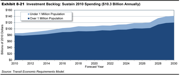
Expansion Investments
In addition to the $10.3 billion spent on transit asset preservation in 2010, transit agencies spent $6.2 billion on expansion investments to support ridership growth and to improve transit performance. This section considers the impact of sustaining the 2010 level of expansion investment on future ridership capacity and vehicle utilization rates under both lower and higher ridership growth rate assumptions. As noted above, it is important to consider here that the $6.2 billion spent on expansion investments in 2010 was significantly higher than that reported in prior years.
As already considered in Chapter 7 (see Exhibit 7-23), the 2010 rate of investment in transit expansion is not sufficient to expand transit capacity at a rate equal to the rate of growth in travel demand, as projected by the historical trend rate of increase. Under these circumstances, it should be expected that transit capacity utilization (e.g., passengers per vehicle) will increase, with the level of increase determined by actual growth in demand. Although the impact of this change may be minimal for systems that currently have lower capacity utilization, service performance on some higher utilization systems would likely decline as riders experience increased vehicle crowding and potential for service delays. This impact is illustrated in Exhibit 8-22, which presents the projected change in vehicle occupancy rates by mode during the period from 2010 through 2030 (reflecting the impacts of spending from 2009 through 2030) under both lower (metropolitan planning organization [MPO]) and higher (trend) rates of growth scenarios in transit ridership, assuming that transit agencies continue to invest an average of $6.2 billion per year on transit expansion. Under the MPO-projected rate of increase, capacity utilization is stable, indicating that investment is sufficient. However, for the higher historical trend rates of increase, there is a steady rise in the average number of riders per transit vehicle across each of the four modes depicted here. For perspective, note that MPO growth rate projections tend to be conservative because they are developed based on financially constrained transportation plans. Moreover, the actual growth in travel demand has typically exceeded the MPO growth projections for much of the past decade.
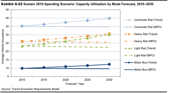
Exhibit 8-23 presents the projected growth in transit riders that can be supported by the 2010 level of investment (keeping vehicle occupancy rates constant) as compared with the potential growth in total ridership under both the lower and higher growth rate scenarios. Similar to prior analyses, the $6.2-billion level of investment for expansion can support ridership growth that is similar to the MPO-projected ridership increases, but is short of that required to support continued ridership growth at recent historical rates (i.e., without impacting service performance).
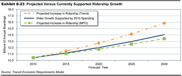
State of Good Repair Benchmark
The preceding scenario considered the impacts of sustaining transit spending at current levels, which appear to be insufficient to address either deferred investment needs (which are projected to increase) or the projected trends in transit ridership (without a reduction in service performance). In contrast, this section focuses on the level of investment required to eliminate the investment backlog over the next 20 years and to provide for sustainable rehabilitation and replacement needs once the backlog has been addressed. Specifically, the SGR benchmark estimates the level of annual investment required to replace assets that currently exceed their useful life, to address all deferred rehabilitation activities (yielding an SGR where the asset has a condition rating of 2.5 or higher), and then to address all future rehabilitation and replacement activities as they come due. The SGR benchmark considered here uses the same methodology as that described in the Federal Transit Administration’s National State of Good Repair Assessment, released June 2010.
| What is the definition of a state of good repair (SGR)? | |
|
The definition of “state of good repair” used for this scenario relies on TERM’s assessment of transit asset conditions. Specifically, for this scenario, TERM considers assets to be in a state of good repair if they are rated at a condition rating of 2.50 or higher and if all required rehabilitation activities have been addressed.
|
|
Differences with Other Scenarios: In contrast to the other scenarios in this chapter, the SGR benchmark (1) makes no assessment of expansion needs and (2) does not apply TERM’s benefit-cost test to investments proposed by TERM. These benchmark characteristics are inconsistent with the SGR concept. First, analyses of expansion investments are ultimately focused on capacity improvements and not on the needs of deteriorated assets. Second, application of TERM’s benefit-cost test would leave some reinvestment needs unaddressed. The intention of this benchmark is to assess the total magnitude of unaddressed reinvestment needs for all transit assets currently in service, regardless of whether it appears to be cost-beneficial for these assets to remain in service.
SGR Investment Needs
Annual reinvestment needs under the SGR benchmark are presented in Exhibit 8-24. Under this benchmark, an estimated $ 18.5 billion in annual expenditures will be required over the next 20 years to bring the condition of all existing transit assets to an SGR. Of this amount, roughly $11.7 billion (63 percent) is required to address the SGR needs of rail assets. Note that a large proportion of rail reinvestment needs are associated with guideway elements (primarily aging elevated and tunnel structures) and rail systems (including train control, traction power, and communications systems) that are past their useful life as well as potentially technologically obsolete. Bus-related reinvestment needs are primarily associated with aging vehicle fleets.
| Asset Type | Urban Area Type | Total | |
|---|---|---|---|
| Over 1 Million Population | Under 1 Million Population | ||
| Rail | |||
| Guideway Elements | $2.8 | $0.1 | $2.9 |
| Facilities | $0.8 | $0.1 | $0.9 |
| Systems | $3.4 | $0.0 | $3.4 |
| Stations | $2.0 | $0.0 | $2.0 |
| Vehicles | $2.5 | $0.0 | $2.5 |
| Subtotal Rail* | $11.4 | $0.3 | $11.7 |
| Nonrail | |||
| Guideway Elements | $0.4 | $0.1 | $0.5 |
| Facilities | $0.9 | $0.7 | $1.6 |
| Systems | $0.2 | $0.0 | $0.2 |
| Stations | $0.1 | $0.0 | $0.1 |
| Vehicles | $3.0 | $1.3 | $4.3 |
| Subtotal Nonrail* | $4.6 | $2.2 | $6.7 |
| Total* | $16.0 | $2.5 | $18.5 |
Exhibit 8-24 also provides a breakout of capital reinvestment needs by type of UZA. This breakout emphasizes the fact that capital reinvestment needs are most heavily concentrated in the Nation’s larger UZAs. Together, these urban areas account for approximately 86 percent of total reinvestment needs (across all mode and asset types), with the rail reinvestment needs of these urban areas accounting for more than one-half of the total reinvestment required to bring all assets to an SGR. This high proportion of total needs reflects the high level of investment in older assets found in these urban areas.
Impact on the Investment Backlog
A key objective of the SGR benchmark is to determine the level of investment required to attain and then maintain an SGR across all transit assets over the next 20 years, including elimination of the existing investment backlog. Exhibit 8-25 shows the estimated impact of the $18.5 billion in annual expenditures under the SGR benchmark on the existing investment backlog over the 20-year forecast period (compare these data with Exhibit 8-21). Given this level of expenditures, the backlog is projected to be eliminated by 2030, with the majority of this drawdown addressing the reinvestment needs of the UZAs with populations greater than 1 million.
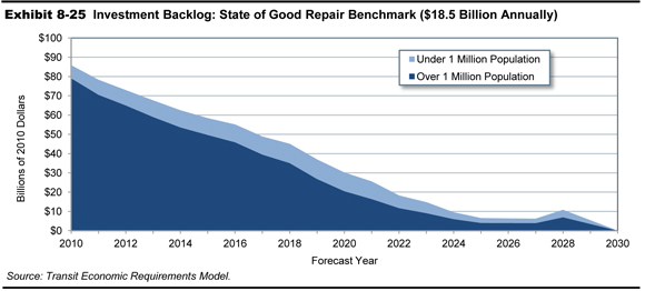
Impact on Conditions
In drawing down the investment backlog, the annual capital expenditures of $18.5 billion under the SGR benchmark would also lead to the replacement of assets with an estimated condition rating of 2.5 or lower. Within TERM’s condition rating system, this includes assets in marginal condition that have ratings of below 2.5 and all assets in poor condition. Exhibit 8-26 shows the current distribution of asset conditions for assets estimated to be in a rating condition of 2.5 or lower (with assets in poor condition segmented into two sub-groups). Note that this graphic excludes both tunnel structures and subway stations in tunnel structures because these are considered assets that require ongoing capital rehabilitation expenditures but that are never actually replaced. As with the investment backlog, the proportion of assets at condition rating 2.5 or lower is projected to decrease under the SGR benchmark from roughly 10 percent of assets in 2010 to well below 1 percent by 2030. Once again, this replacement activity would remove from service those assets with higher occurrences of service failures, technological obsolescence, and lower overall service quality.
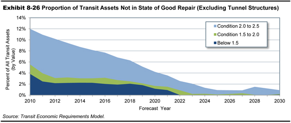
Impact on Vehicle Fleet Performance
While the preceding analysis considered the impact of higher investment on reducing the investment backlog and potential replacement of assets past their useful life, this analysis may not provide a sense of the potential positive implications of these changes for daily transit service. To help better understand these effects, Exhibit 8-27 shows the estimated percent reduction in fleet-wide revenue service disruptions (relative to 2010) for heavy rail and motor bus vehicles resulting from the retirement of over-age transit passenger vehicles under the SGR benchmark. Note that the large variation in the percent reduction for bus is a result of the timing of large bus fleet replacements. Also, while the reduction in service disruptions is significant for bus and heavy rail vehicles, some vehicle types (e.g., light and commuter rail) actually show a net increase in service disruptions under the SGR benchmark; this is because the current age distribution for these fleets is skewed toward younger vehicle ages and is not sustainable in the longer term. This effect is the result of the recent development of new light rail and commuter rail systems.
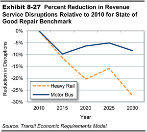
Low and High Growth Scenarios
The preceding scenario considered the level of investment to bring existing transit assets to a SGR but in doing so did not consider either (1) the cost effectiveness of these investments (investments were not required to pass TERM’s benefit-cost test) or (2) the level of expansion investment required to support projected ridership growth. The Low Growth scenario and High Growth scenario address both of these issues. Specifically, these scenarios use the same rules to assess when assets should be rehabilitated or replaced as were applied in the preceding SGR benchmark (e.g., with assets being replaced at condition 2.5), but also require that these preservation and expansion investments pass TERM’s benefit-cost test. In general, some reinvestment activities do not pass this test (i.e., have a benefit-cost ratio of less than one), which can result from low ridership benefits, higher capital or operating costs, or a mix of these factors. Excluding investments that do not pass the benefit-cost test has the effect of reducing total estimated needs.
In addition, the Low and High Growth scenarios also assess transit expansion needs given ridership growth as projected by the Nation’s MPOs (low growth) and based on the average annual compound rate as experienced over the last 15-year period (high growth). For the expansion component of this scenario, TERM assesses the level of investment required to maintain current vehicle occupancy rates (at the agency-mode level) subject to the rate of projected growth in transit demand in that UZA and also subject to the proposed expansion investment passing TERM’s benefit-cost test.
Low Growth Assumption
The Low Growth scenario is intended to provide a lower bound on the level of investment required to maintain current service performance (as measured by transit vehicle capacity utilization) as determined by a relatively low rate of growth in travel demand. In particular, this Low Growth scenario relies on growth in travel demand as projected by a sample of the MPOs (representing the Nation’s 30 largest UZAs and a sample of smaller UZAs). When aggregated across the Nation’s UZAs (and corrected for differences in transit demand by UZA), this source yields a national average annual growth rate of 1.4 percent over the 20-year period from 2010 to 2030. (This represents the weighted average growth rate at the national level. In practice, the ridership growth rates applied by TERM vary by UZA based on the growth projections obtained from that UZA’s MPO.) This projected rate of growth is less than the 2.2-percent trend rate experienced over the 15 year period from 1995 to 2010 (as utilized by the High Growth scenario presented below), but is higher than the 1.2 percent trend rate of growth in urban population over the decade from 2000 to 2010 (a primary driver of transit ridership).
The MPO projections are considered low (or at least conservative) for the following reasons. First, MPO transit demand projections are financially constrained (i.e., projected ridership growth is limited by the expected capacity to fund expansion projects) and, hence, these projections are lower than the potential for increased ridership demand if funding were unconstrained. Second, as discussed further in Chapter 9, the historical rate of increase in transit ridership and transit passenger miles have generally exceeded MPO growth projections for these same time periods, again tending to characterize the MPO growth projections as relatively low or conservative.
High Growth Assumption
The High Growth scenario provides a higher bound on the level of investment required to maintain current service performance as determined by a relatively high rate of growth in travel demand. In particular, the High Growth scenario relies on the trend rate of growth in transit passenger miles over the period 1995 through 2010 as reported to the NTD. When calculated across all transit operators, this historical trend rate of growth converts to a national average compound annual growth rate of 2.2 percent during this time period. Similar to the MPO growth rates in the Low Growth scenario, the 15-year trend growth rates applied by TERM for the High Growth scenario also vary by UZA either based on the actual trend rates of growth experienced by each UZA (for UZAs close to or higher than 1 million in population) or based on the average for UZAs of comparable size in the same geographic region. This rate is considered relatively high primarily due to the unusually high rate of growth in ridership experienced over the period from roughly 2006 to 2010, partly in response to high fuel prices.
Low and High Growth Scenario Needs
TERM’s projected annual average capital investment needs under the Low and High Growth scenarios—including those for both asset preservation and asset expansion—is presented in Exhibit 8-28.
| Asset Type | Lower Growth | Total | Higher Growth | Total | ||
|---|---|---|---|---|---|---|
| Preservation | Expansion | Preservation | Expansion | |||
| Rail | ||||||
| Guideway Elements | $2.7 | $0.7 | $3.5 | $2.8 | $0.9 | $3.6 |
| Facilities | $0.9 | $0.1 | $0.9 | $0.9 | $0.1 | $1.0 |
| Systems | $3.4 | $0.2 | $3.5 | $3.4 | $0.2 | $3.6 |
| Stations | $1.8 | $0.5 | $2.2 | $1.8 | $0.6 | $2.4 |
| Vehicles | $2.5 | $0.8 | $3.3 | $2.5 | $1.3 | $3.8 |
| Other Project Costs | $0.0 | $0.7 | $0.7 | $0.0 | $0.9 | $0.9 |
| Subtotal Rail* | $11.2 | $2.9 | $14.2 | $11.3 | $4.0 | $15.3 |
| Nonrail | ||||||
| Guideway Elements | $0.4 | $0.1 | $0.5 | $0.4 | $0.1 | $0.5 |
| Facilities | $1.4 | $0.3 | $1.7 | $1.4 | $0.6 | $2.0 |
| Systems | $0.2 | $0.0 | $0.3 | $0.2 | $0.1 | $0.3 |
| Stations | $0.1 | $0.0 | $0.1 | $0.1 | $0.0 | $0.1 |
| Vehicles | $4.0 | $1.2 | $5.3 | $4.1 | $2.3 | $6.3 |
| Other Project Costs | $0.0 | $0.0 | $0.0 | $0.0 | $0.0 | $0.0 |
| Subtotal Nonrail* | $6.1 | $1.7 | $7.8 | $6.1 | $3.1 | $9.2 |
| Total Investment* | $17.3 | $4.6 | $22.0 | $17.4 | $7.1 | $24.5 |
Lower Growth Needs
Assuming the relatively low ridership growth in the Low Growth scenario, total investment needs for both system preservation and expansion are estimated to average roughly $22.0 billion each year for the next two decades. Of this amount, roughly 79 percent are for preservation of existing assets and approximately $11 billion is associated with preservation of existing rail infrastructure alone. Note that the $1.2 billion difference between the $18.5 billion in annual preservation needs under the SGR benchmark and the $17.3 billion in preservation needs under the Low Growth scenario is entirely due to the application of TERM’s benefit-cost test under the Low Growth scenario. Finally, expansion needs in this scenario total $4.6 billion annually, with 63 percent of that amount associated with rail expansion costs.
Higher Growth Needs
In contrast, total investment needs under the High Growth scenario are estimated to be $24.5 billion annually, a 12 percent increase over the total investment needs under the Low Growth scenario. The High Growth scenario total includes $17.4 billion for system preservation and an additional $7.1 billion for system expansion. Note that system preservation costs are higher under the High Growth scenario because the higher growth rate leads to a larger expansion of the asset base as compared to the Low Growth scenario. Under this scenario, investment in expansion of rail assets is still larger than that for nonrail expansion (56 percent for rail and 44 percent for non-rail). However, under the High Growth scenario rail takes only 56 percent of total expansion investment versus 63 percent of expansion needs under the Low Growth scenario. Overall, total expansion investment needs are roughly 53 percent higher for the High Growth scenario than for the Low Growth scenario (which is somewhat consistent with the high growth rate at 2.2 percent being approximately 60 percent higher than the low growth rate of 1.4 percent).
Impact on Conditions and Performance
The impact of the Low and High Growth Rate preservation investments on transit conditions is essentially the same as that already presented for the SGR benchmark in Exhibit 8-25 and Exhibit 8-26. As noted above, these scenarios use the same rules to assess when assets should be rehabilitated or replaced as were applied in the SGR benchmark (e.g., with assets being replaced at condition rating 2.5). In terms of asset conditions, the primary difference between the SGR benchmark and the Low and High Growth scenarios relates to: (1) TERM’s benefit-cost test not applying to the SGR benchmark (leading to higher SGR preservation needs overall) and (2) the Low and High Growth scenarios having some additional needs for the replacement of expansion assets with short service lives. Together, these impacts tend to work in opposite directions with the result that the rate of drawdown in the investment backlog and the elimination of assets exceeding their useful life are roughly comparable for each of these three scenarios.
Similarly, the impact of the Low and High Growth rate expansion investments on transit performance was considered in Exhibit 8-23. That analysis demonstrated the significant difference in the level of ridership growth supported by the High Growth scenario as compared with either the current level of expenditures ($5.4 billion in 2010 for UZAs over 1 million) or the rate of growth supported under the Low Growth scenario.
Scenario Benefits Comparison
Finally, this subsection summarizes and compares many of the investment benefits associated with each of the four analysis scenarios considered above. While much of this comparison is based on measures already introduced above, this discussion also considers a few additional investment impact measures. These comparisons are presented in Exhibit 8-29. Note that the first column of data in Exhibit 8-29 presents the current values for each of these measures (as of 2010). The subsequent columns present the estimated future values in 2030 assuming the levels, allocations, and timing of expenditures associated with each of the four investment scenarios.
Exhibit 8-29 includes the following measures:
- Average Annual Expenditures (billions of dollars): This amount is broken down into preservation and expansion expenditures.
- Condition of Existing Assets: This analysis only considers the impact of investment funds on the condition of those assets currently in service.
Average Physical Condition Rating: The weighted average condition of all existing assets on TERM’s condition scale of 5 (excellent) through 1 (poor).
Investment Backlog: The value of all deferred capital investment, including assets exceeding their useful lives and rehabilitation activities that are past due (this value can approach but never reach zero due to assets continually aging with some exceeding their useful life). The backlog is presented here both as a total dollar amount and also as a percent of the total replacement value of all U.S. transit assets.
Backlog Ratio: The ratio of the current investment backlog to the annual level of investment required to maintain normal annual capital needs once the backlog is eliminated
. - Performance Measures: The impact of investments on U.S. transit ridership capacity and system reliability.
New Boardings Supported by Expansion Investments: The number of additional riders that transit systems can carry without a loss in performance (given the projected ridership assumptions for each scenario).
Carbon Dioxide (CO2) Emissions Avoided (millions of metric tons): Potential reduction in CO2 emissions from providing the additional transit rider carrying capacity (assumes that riders would otherwise use other modes of travel, including automobiles).
Revenue Service Disruptions per Passenger Mile Traveled: Number of disruptions to revenue service per million passenger miles.
Fleet Maintenance Cost per Vehicle Revenue Mile: Fleet maintenance costs tend to increase with fleet age (or reduced asset condition). This measure estimates the change in fleet maintenance costs expressed in a per-revenue-vehicle-mile basis.
| Measure | Baseline 2010 Actual Spending, Conditions and Performance | Scenarios for 2030 | |||
|---|---|---|---|---|---|
| Sustain 2010 Spending | SGR | Low Growth | High Growth | ||
| Average Annual Expenditures (Billions of 2010 Dollars) | |||||
| Preservation | $10.3 | $10.3 | $18.5 | $17.3 | $17.4 |
| Expansion | $6.2 | $6.2 | NA | $4.6 | $7.1 |
| Total | $16.5 | $16.5 | $18.5 | $22.0 | $24.5 |
| Conditions (Existing Assets) | |||||
| Average Physical Condition Rating | 3.75 | 3.39 | 3.54 | 3.54 | 3.54 |
| Investment Backlog (Billions of Dollars) | $85.9 | $141.7 | $0.0 | $0.0 | $0.0 |
| Investment Backlog (% of Replacement Costs) | 12.6% | 20.9% | 0.0% | 0.0% | 0.0% |
| Backlog Ratio1 | 6.1 | 10.0 | 0.0 | 0.0 | 0.0 |
| Performance | |||||
| Ridership Impacts of Expansion Investments (2010) | |||||
| New Boardings Supported by Expansion (Billions) | NA | 4.6 | NA | 3.0 | 5.4 |
| CO2 Emissions Avoided (Millions of Metric Tons) | NA | 3.0 | NA | 1.9 | 3.5 |
| Fleet Performance | |||||
| Revenue Service Disruptions per Thousand PMT | 9.5 | 10.5 | 9.3 | 9.2 | 9.3 |
| Fleet Maintenance Cost per Revenue Vehicle Mile | $1.75 | $1.86 | $1.74 | $1.73 | $1.73 |
| Other Benefits | |||||
| Job Years Impact (Thousands)2 | |||||
| Operating and Maintenance | 1,201.7 | 1,620.6 | 1,201.7 | 1,549.3 | 1,828.4 |
| Capital | 264.3 | 264.3 | 295.4 | 351.3 | 392.6 |
| Total Annual Job Years Supported | 1,466.0 | 1,884.9 | 1,497.0 | 1,900.6 | 2,221.0 |
| GDP Impact (Billions of Dollars) | |||||
| Operating and Maintenance | $71.1 | $95.9 | $71.1 | $91.7 | $108.2 |
| Capital | $22.0 | $22.0 | $24.6 | $29.3 | $32.7 |
| Total Annual Incremental Impact | $93.1 | $117.9 | $95.7 | $120.9 | $140.9 |
2 Includes direct, indirect, and induced impacts.
- Other Benefits: Impacts other than those to transit conditions and performance. The jobs and Gross Domestic Product (GDP) impacts considered here were determined using an input-output analysis.
Jobs Impacts: The number of job years associated with both transit mode operations and ongoing capital investment (both preservation and expansion), including direct, indirect, and induced job years. Each $1 million invested in transit operation activities is estimated to support 33 job years while each $1 million invested in transit capital investments supports 16 job years.
GDP Impacts: The impact on GDP associated with both transit mode operations and ongoing capital investment (both preservation and expansion), including direct, indirect, and induced impacts. Each $1 invested in transit operation activities is estimated to generate $0.95 in additional GDP while each $1 invested in transit capital investments generates $0.33 in additional GDP.
Scorecard Comparisons
A review of the scorecard results for each of the four investment scenarios reveals the impacts discussed below.
Preservation Impacts
Continued reinvestment at the 2010 level is likely to yield a decline in overall asset conditions, an increase in the size of the investment backlog, and an increase in both service disruptions per million passenger miles and in maintenance costs per vehicle revenue mile. In contrast, with the exception of overall asset conditions, each of these measures is projected to improve under the SGR, Low Growth, and High Growth scenarios, each of which project roughly comparable levels of required capital reinvestment expenditures. Note that the overall condition rating measure of 3.54 under these last three investment scenarios represents a sustainable, long-term condition level for the Nation’s existing transit assets over the long term (in contrast to the current measure of roughly 3.8, which would be difficult to maintain in the long term without replacing many asset types prior to the conclusion of their expected useful lives).
Expansion Impacts
While continued expansion investment at the 2010 level appears sufficient to support a relatively low rate of increase in transit ridership, recent historical rates of growth suggest that a significantly higher rate of expansion investment is required to avoid a decline in overall transit performance (e.g., in the form of increased crowding on high utilization systems). Higher rates of transit expansion investment, as required to support higher transit ridership growth or through a shift from auto travel to transit, can also help yield reductions in CO2 emissions. Finally, higher rates of expansion investment also tend to support higher direct, indirect and induced impacts on jobs and other economic activity related to transit operations, construction, and rehabilitation activities.