Using Falling Weight Deflectometer Data With Mechanistic-Empirical Design and Analysis, Volume II: Case Study Reports

CHAPTER 6.

CASE STUDY 6: COMPOSITE PAVEMENT EVALUATION AND OVERLAY DESIGN

PROJECT OVERVIEW

Project 19-0600 from the LTPP Program SPS-6 database served as the basis for the composite pavement case study. The 19-0600 project was located on I-35 near Des Moines, IA, and test section 19-0659 was selected for the indepth analysis. Test section 19-0659 was a composite pavement cross section with an HMA surface (overlay) on a JRCP and granular base layer over subgrade. This section is representative of the following selection factors:

• Composite pavement.
• Wet-freeze climate zone.
• Principal arterial—interstate (rural) functional class.
• “Fair” pavement condition.
• Clay subgrade classification.
• No (or deep) rigid layer.

The original JRCP pavement, nominally a 10-inch (254-mm) PCC slab on a 8-inch (203.2-mm) base with 76.5-ft (23.3-m) transverse joint spacing, was constructed about 1965. A 4‑inch (101.3-mm) HMA overlay was placed in 1989. In addition, the LTPP Program database indicates that a number of different maintenance activities were conducted over the years, including asphalt crack sealing in 1990, full-depth transverse joint repair patching in 1992, full-depth patching of HMA pavement in 1999, and skin patching in 2006. Although the existing PCC pavement is a jointed reinforced design, the MEPDG software did not, at the time of this report, differentiate between plain and reinforced pavement in the rehabilitation process.

PAVEMENT CONDITION/PERFORMANCE

Pavement condition and performance data can be used to customize (or calibrate) the performance models within the MEPDG software for the specific highway agency using the design program. However, the calibration of performance models was beyond the scope of this study. Therefore, the difference in predicted distress and rehabilitation results based on the globally calibrated models were compared for backcalculation-based and laboratory-based inputs.

The inputs used in the pavement rehabilitation design used relatively little distress data. The distress data used for design inputs of HMA overlay rehabilitation of JPCP (including composite pavements) consisted of the percentage of cracked slabs before rehabilitation and the percentage of slabs repaired. The MEPDG design software does not directly analyze JRCP; however, it was assumed that the reinforcement held cracks tight so that they would not reflect through the overlay. Documenting the distress data for the underlying slabs in a composite pavement is problematic for design, even if the existing HMA overlay is intended to be milled off during rehabilitation. In addition, for a composite pavement, reflective cracking is a critical distress that must be considered. The MEPDG reflective cracking model accounts for two modes of crack formation: propagation of existing cracks and propagation of new cracks. While the new cracking was estimated within the program, the documentation was not clear on how the number of existing cracks was determined. There was no distress input for the structure as in many of the other design types (figure 88), but the “Rehabilitation” input screen (figure 89) allows entering the percent of cracked slabs before and after restoration activities. However, based on the results of the design runs, there appears these inputs had little influence.

1 inch = 25.4 mm.
Figure 88. Screen Capture. Structure input screen for HMA over JPCP rehabilitation.

1 psi/inch = 0.263 kPa/mm.
Figure 89. Screen Capture. Existing distress input in “Rehabilitation” screen.

The MEPDG also recommended that the backcalculated PCC modulus be adjusted in relation to the general slab conditions. Again, assessing the general slab conditions was problematic for a composite pavement. Therefore, judgment was required in relating HMA surface distresses and the condition of the pavement before overlay, if available, to the general condition of the underlying PCC during the design process.

Visual distress data were not available in the LTPP Program database for the original JRCP; however, both manual survey data and photographic survey data were available for the HMA surface for several years between 1989 and 2007. As mentioned previously, one of the primary distresses of concern in composite pavements was reflective cracking, but this distress was not specifically identified in the LTPP Program database. Reflective cracking was included in the transverse cracking distress quantity, which also may include thermal cracking of the HMA overlay.

Figure 90 shows the development of transverse cracking since the placement of the HMA overlay in 1989 (based on either manual or photographic surveys). The research team assumed that the absence of cracking in 2005 and 2007 was due to repairs conducted in the interim years. The manual survey recorded 30 cracks in 2001, while the photographic survey recorded 115cracks; based on the general progression, 30 cracks was more probable. With the section approximately 500 ft (152.5 m) long and a joint spacing of approximately 76.5 ft (23.3 m), there were approximately 6.5 slabs. There would be approximately 4 to 5 cracks (including reflective cracks over the joints) per slab assuming 30 cracks for the section.

1 ft = 0.305 m.
Figure 90. Graph. Summary of transverse cracking distress data for test section 19-0659.

The distresses that were identified in the 2007 data for the HMA surface are summarized in table 88. These distresses included alligator and block cracking, patching, and one location of water bleeding.

TEST SECTION DATA

The MEPDG design program requires a significant number of inputs. The required design data for test section 19-0659 were obtained from the LTPP Program DataPave database. The required data were not generally complete for any one specific test section within project 19‑0600; therefore, results from the entire project were used to obtain the necessary design inputs. While the test sections had slightly different cross sections and maintenance histories, the research team concluded that the data were sufficient for the purposes of this study.

Deflection-Testing Data.

Deflection data for test section 19-0659 were available from the LTPP Program database for several years of testing between 1989 and 2007. In addition, laboratory testing data for the PCC layer were available from 2007. Because the 2007 deflection data were the most recent, and there was corresponding PCC testing for that year, the deflection data from 2007 were used in this analysis.

Equipment

Deflection testing was conducted with a Dynatest® FWD (SN 8002-129 for 2007 dataset).

Sensor Configuration

Sensors were located at 0,8, 12, 18, 24, 36, 48, 60, and -12 inches (0, 203.2, 304.8, 457.2, 609.6, 914.4, 1,219.2, 1,524, and -304.8 mm) for data collected during 2007.

Number of Drops and Load Levels

Four load level targets—6,000, 9,000, 12,000, and 16,000 lb (2,724, 4,086, 5,448, and 7,264 kg)—with four drops at each load level were performed, and the resultant data recorded. Seating drops were also performed at each load level, but the deflection data were not recorded. Time histories were also available for the fourth drop height.

Test Locations/Lanes and Increments

Testing was conducted mid-lane and in the outer wheelpath at approximately 40- to 80-ft (12.2- to 24.4-m) intervals.

Temperature Measurements

During the deflection testing, temperature measurements were taken at predetermined time intervals using drilled holes in the composite pavement at depths of 0.9, 2.2, 3.8, 8.2, and 12.0inches (22.9, 55.9, 96.5, 208.3, and 304.8 mm) below the pavement surface.

Material Properties Data.

This section summarizes the data obtained from the LTPP database for test section 19-0659 regarding its subgrade, granular base, HMA and PCC material properties, traffic, climate, and depth of water table or stiff layer.

Subgrade

Six subgrade samples were retrieved from the 19-0600 project location, including two samples from test section 19-0659, as part of the LTPP Program. The subgrade was generally classified as A-4 to A-6 materials under the AASHTO soil classification system.⁽²⁾

Laboratory resilient modulus testing results were available for the six samples of the subgrade materials obtained as part of the LTPP Program data collection; however, one sample’s results were significantly different than the remaining samples and were not included in this analysis. Laboratory resilient modulus testing results for the subgrade samples (identified as TS##) evaluated are illustrated in figure 91.

1 psi = 6.89 kPa.
Figure 91. Graph. Summary of LTPP Program laboratory measured resilient modulus for collected subgrade samples.

Additional subgrade properties, including Atterberg limits and sieve analysis, are summarized in table 89 and table 90, respectively.

Granular Base

Laboratory resilient modulus testing for the granular base material for project 19-0600 was not available. The base was classified as an uncrushed gravel, and the Atterberg limits generally indicate the material was nonplastic. Aggregate sieve analysis of the base aggregate is summarized in table 91.

PCC Pavement

PCC data available from the LTPP Program database included unit weight, compressive strength, splitting tensile strength, and elastic modulus testing from cores tested in 2007. In addition, the CTE testing was conducted on retrieved cores. The available PCC properties are summarized in table 92 through table 94.

Table 91. Summary of base aggregate sieve analysis.

Table 94. Summary of PCC pavement design features.

Although the joint spacing was 76.5 ft (23.3 m), the MEPDG design program did not allow joint spacing greater than 25 ft (7.6 m). Even when setting a 25-ft (7.6-m) joint spacing, a program warning was encountered indicating that 20 ft (6.1 m) was the acceptable maximum spacing. (Note that the newer version 1.1 of the design software now allows up to a 30-ft (9.1 m) joint spacing.)

HMA Surface

Information for the existing HMA overlay included aggregate gradation and general mix properties. Asphalt cement grading was obtained from adjacent LTPP General Pavement Studies sections; an AC-20 was used for the last surface layer constructions. The available existing HMA overlay properties are summarized in table 95 and table 96. Resilient modulus testing for the existing HMA overlay was also conducted and is summarized in figure 92.

Table 95. Summary of existing HMA material properties.

Table 96. Summary of existing HMA aggregate sieve analysis.

1 psi = 6.89 kPa.
°F = 1.8 × °C + 32.
Figure 92. Graph. Summary of HMA resilient modulus testing.

Based on the laboratory data, the existing HMA binder and surface layers had relatively similar resilient moduli, with an average instantaneous resilient modulus of approximately 1,460,000 psi (10,059,400kPa) at 70 °F (21.1 °C) and an average total resilient modulus of approximately 3,880,000 psi (26,733,200 kPa) at 70 °F (21.1 °C), both of which were quite high for HMA.

Depth to Rigid Layer/Water Table.

The depth to the water table is another input required for the MEPDG. However, no data were found for project 19-0600. One record was obtained from the LTPP Program database for Iowa, indicating the depth to a rigid layer was greater than 100 ft (30.5 m). Records also suggested a perched water table was possible between April and July at a depth of 12 to 48 inches (304.8 to 1219.2 mm). Historical groundwater levels from the USGS indicated an average of approximately 12 ft (3.7 m) below land surface.⁽⁴⁾

Climate/Environment Data.

Climate data were obtained from the updated climate files on the MEPDG Web site.⁽⁵⁾ The weather station at Des Moines, IA, was used for this study. The general climatic category for the case study location is wet-freeze.

Traffic Data

Traffic data were obtained from the LTPP Program database. Because evaluating the effect of traffic data on design results was not a primary goal of this study, only basic information was used from the available data (total volume, growth, and vehicle class distribution), with the remaining inputs (such as monthly distribution, hourly distribution, and wheel spacing) kept at their default values in the MEPDG software. A 2.15-percent linear growth was estimated based on traffic data from 1965 to 1993. An initial two-way AADTT volume of 6,179 vehicles per day for 2009was estimated based on the linear estimation. The vehicle class distribution obtained from the LTPP Program database is summarized in table 97.

Table 97. Traffic distribution by vehicle class.

ANALYSIS AND INTERPRETATION OF FWD TESTING DATA

This section presents the data checks and backcalculation analysis of the FWD data, as well as a comparison of the backcalculation results with laboratory testing.

Preprocessing Deflection Data.

Before conducting the backcalculation analysis, prescreening of the data was accomplished in a spreadsheet format to identify any outlying or questionable data. An examination of the 2007data revealed a number of locations with non-decreasing deflections. Although these points were potentially recorded, they were generally not included in a backcalculation analysis. However, for test section 19-0659, 6 of the 10 test locations had non-decreasing basins for one or more of the test drops, and it was generally recommended that 25 percent or fewer of the data points should be removed before questioning the entire dataset. For this case study, only the non-decreasing deflection basin locations were used in estimating the k-value and PCC modulus even though this resulted in removal of more than 25 percent of the locations.

Next, a review of the normalized deflections of the entire dataset to a load level of 9,000 lb (4,086 kg) (impulse stiffness modulus can also be used) was performed to evaluate whether the load response was relatively uniform along the tested section or whether the pavement should be divided into smaller sections. The normalized deflection plot for the 2007 dataset is illustrated in figure 93. From this plot, the deflections appear relatively uniform, with only a slight difference between the normalized deflections for the different load levels. Table 98 summarizes the 9,000‑lb (4,086‑kg) normalized deflections associated with each load level.

1 mil = 0.0254 mm.
1 lb = 0.454 kg.
1 ft = 0.305 m.
Figure 93. Graph. Normalized deflection plot for 2007 mid-lane deflection basins.

Backcalculation Analysis.

Backcalculation of the 19-0659 deflection data was performed using the outer-AREA method with the SHRP five-sensor equations to determine the k-value and layer moduli. The outer-AREA method was used to account for compression in the HMA overlay of the composite pavement structure. The analysis consisted of a three-layer system: HMA overlay, PCC slab, and spring foundation.

Backcalculation Results

The average results from the backcalculation are summarized in table 99. The variability in the k‑value was relatively low, and while the variability in the bound layers was higher, it was still acceptable. In this case, the foundation represented the granular base and subgrade. The determined k-value using the outer-AREA method would also include the effects of a rigid layer, if present.

The outer-AREA method was first used to calculate an effective modulus of a single plate with an equivalent thickness equaling the combined thickness of the two layers. The HMA overlay and PCC slab moduli were then determined following the relationship developed by Ioannides and Khazanovich for a two-plate system (the layers are assumed to be bonded).⁽¹⁵⁾ The determination of the individual layer moduli requires the assumption of a modular ratio (β) of the PCC and HMA moduli. A typical modular ratio for a dense-graded HMA is 10 and was used in the initial backcalculation results.⁽¹⁶⁾ However, a range of modular ratios are summarized in with corresponding HMA and PCC moduli. As shown in Table 100, the HMA modulus was more sensitive to the modular ratio selection, increasing by 100 percent from a ratio of 10 to a ratio of 4, while the PCC modulus decreased only by 25 percent over that range.

Backcalculation Modeling Issues and Recommendations

The existing pavement structure was considered a four-layer system (five-layer system if a rigid layer were present). The aggregate base layer was included in the determined k-value, as was the presence of any rigid layer. In addition, an effective modulus for an equivalent single plate was first determined, and the individual bound layer moduli were then determined using a modular ratio. The closed-form solutions for composite pavements at the time of this report were not well suited for more than two bound layers and multiple unbound layers.

Comparison of Backcalculation and Laboratory Testing Results.

To assist in evaluating which layer characteristics were appropriate to use in the MEPDG software, the results of the backcalculation (field tests) were compared with results obtained from laboratory testing conducted as part of the LTPP Program. While it was outside of the scope of this study to develop new correlations or conversion factors between the two, it was still beneficial to evaluate these relationships and how they may influence MEPDG input selection.

Unbound Materials

The first general argument when comparing field with laboratory results of unbound materials is the stress state of the material is different for the two conditions. To compare laboratory results with those obtained from FWD testing (or vice versa), the resilient modulus was estimated for the stress conditions at the time of FWD testing. The stress conditions accounted for the overburden pressure of the pavement and the stress due to loading. Laboratory testing was only available for the subgrade material for 19-0600, so only the subgrade comparison was discussed in this case study.

Load stresses were determined using ILLISLAB, the load applied during deflection testing, and initial backcalculated layer properties. Overburden stresses were estimated using layer densities, moisture contents, thicknesses, and at-rest earth pressure coefficient (K₀). K₀ for fine-grained unbound layers was estimated using the equation in figure 94.

Figure 94. Equation. Estimation for at-rest earth pressure coefficients for fine-grained unbound layers.

Where:

K₀ = At-rest earth pressure coefficient.
v = Poisson’s ratio.

To compare the resilient modulus at the stress conditions of FWD testing, the constitutive model in figure 95 (contained in the MEPDG) was used.⁽⁶⁾

Figure 95. Equation. Constitutive model for determining resilient modulus.

Where:

M_R = Resilient modulus, psi (kPa).
k₁, k₂, k₃ = Regression constants.
p_ɑ = Atmospheric pressure, psi (kPa).
θ = Bulk stress, psi (kPa).
τ_Oct = Octahedral shear stress, psi (kPa).

The constitutive model coefficients determined for the subgrade materials from available laboratory results for the 19-0600 project are summarized in table 101; the model is illustrated in figure 96, where TS** designates the respective samples. Figure 97 illustrates the fit of the constitutive model with the measured properties.

Table 101. Summary of estimated subgrade constitutive regression constants.

1 psi = 6.89 kPa.
Figure 96. Graph. Estimated constitutive model for subgrade resilient modulus.

1 psi = 6.89 kPa.
Figure 97. Graph. Comparison of subgrade laboratory resilient modulus with predicted resilient modulus.

Although moisture condition influenced the resulting resilient modulus, laboratory resilient modulus testing was conducted at the in situ conditions, and only a general comparison of values is intended here, so the specific effects of moisture were not considered in this case study.

The backcalculation procedures for rigid pavements provided a k-value, whereas the laboratory testing of material samples resulted in the determination of a resilient modulus value. One available correlation for k-value and resilient modulus is shown in figure 98.⁽²⁾

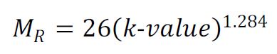
Figure 98. Equation. Correlation for k-value and resilient modulus.

Where:

M_R = Resilient modulus, psi.
k-value = Modulus of subgrade support, psi /inch.

However, the k-value determined using the outer-AREA backcalculation was a dynamic k-value and included the contribution of the unbound base layer as well as the subgrade (and bedrock, if present). A factor of 0.5 is commonly applied to convert a dynamic k-value to a static k-value. So, for this section the dynamic k-value corresponded to a static composite k-value of approximately 95 psi /inch (26 kPa/mm) and a resilient modulus of 9,000 psi (62,010 kPa). These values were considered somewhat low for a composite material that included the effects of both the subgrade and the aggregate base materials.

Determination of individual layer properties from the composite k-value was a more difficult task. One possible solution was to use the PCA’s forward design procedure for determining the influence of an aggregate base layer on a subgrade k-value for use in slab thickness design.⁽¹³⁾ In this case, the improved k-value was used to back out a subgrade k-value for the thickness of the aggregate layer. Using this method, the research team found that the subgrade static k-value was approximately 62 psi/inch (17 kPa/mm), which corresponds to a subgrade resilient modulus of approximately 5,300 psi (36,517 kPa). A modulus value for the base layer would then need to be assumed (values of 25,000 to 35,000 psi (172,250 to 241,150 kPa)) were used in the design analyses, as discussed later). Another possible solution could be obtained using layered elastic analysis to match the measured deflections, similar to the conversion for new rigid pavement design within the MEPDG software. This method would also require some assumptions for the base layer modulus to determine the subgrade modulus. This latter approach was not investigated for this case study, however.

The estimated subgrade resilient modulus based on laboratory testing and using the constitutive model at the stress conditions for a 9,000-lb (4,086-kg) FWD load was 14,900 psi (102,661 kPa). This was much higher than the estimated subgrade modulus and the composite modulus based on the backcalculated k-value. However, it was quite close to the default design input for the material type (14,000 psi (96,460 kPa)).

Using the k-value-to-resilient modulus correlation in figure 95, a dynamic-to-static (composite value) k-value correction of 0.74 (instead of the 0.5 correction) would provide more consistent values in this case. However, the correlation equation for k-value to resilient modulus may as likely be the source of the observed difference.

To assess the significance of determining appropriate correction factors, several combinations of k-value and layer modulus were evaluated, as discussed later in this case study.

Bound Materials

This section presents results of the comparison of the backcalculation results from both PCC and HMA overlay layers with laboratory test results.

PCC Layer

For the PCC surface, the splitting tensile strength, compressive strength, and elastic modulus testing results were available for cores retrieved for section 19-0600. The testing values were converted to elastic modulus and flexural strength estimates using the respective correlation equations summarized in figure 99, with the calculations summarized in table 102.⁽⁶⁾

Figure 99. Equation. Various strength and elastic modulus correlation equations.

Where:

E_pcc = Elastic modulus, psi (kPa).
MR = Flexural strength, psi (kPa).
ρ = Density of PCC (2.18 g/cm³ (136 lb/ft³⁾ from LTPP Program data).
f'_c = Compressive strength, psi (kPa).
ƒ_t = Splitting tensile strength, psi (kPa).

While the estimated elastic modulus from the compressive strength testing was fairly similar to the measured elastic modulus, the estimated elastic modulus from the splitting tensile strength was quite a bit higher.

The elastic modulus obtained from backcalculation is a dynamic value, one that is based on a rapid, relatively low stress level. As such, it cannot be compared directly with the elastic modulus obtained through laboratory testing. Typically, an adjustment factor of 0.8 has been historically recommended for converting a backcalculated PCC elastic modulus value to a static elastic modulus value.⁽⁶⁾ The static PCC modulus values are summarized in table 103 for varying modular ratios, showing that the moduli were still greater than those based on laboratory testing. Adjustment factors ranged from approximately 0.39 to 0.86 depending on modular ratio and laboratory testing result.

HMA Overlay Layer

The estimated HMA modulus at 70 °F (21.1 °C) based on laboratory testing was approximately 3,880,000 psi (26,733,200 kPa) (total resilient modulus), which was extremely high for an HMA material. The estimate of the laboratory-based HMA modulus for a temperature of 87 °F (30.6 °C) (average temperature at the time of FWD testing) was 2.2 million psi (15,158,000kPa), which was significantly greater than the backcalculated value (852,500 psi (5,873,725 kPa) using a modular ratio of 10). Alternatively, the backcalculated HMA modulus can be adjusted for temperature based on the equation in figure 100.⁽¹⁷⁾

Figure 100. Equation. Asphalt temperature adjustment factor.

Where:

ATAF = Asphalt temperature adjustment factor.
slope = Slope of the log modulus versus temperature equation (-0.021 for mid-lane).
T_r = Reference HMA mid-depth temperature °F (°C).
T_m = HMA mid-depth temperature at time of testing °F (°C).

A correction factor of approximately 1.66 was estimated using the last equation in figure 99 for a reference temperature of 70 °F (21.1 °C). The temperature-corrected HMA moduli for a range of modular ratios are summarized in Table 104. Summary of temperature corrected HMA modulus.

An additional consideration in comparing laboratory and deflection testing is the frequency of loading. Laboratory resilient modulus testing is conducted with a 0.1-s load pulse, whereas FWD testing is conducted with a 0.03-s load pulse (approximately). Although dynamic modulus testing data were not available, reviewing the approach for shifting the HMA modulus due to frequency and temperature was worthwhile. Based on the available HMA properties, recommended MEPDG default values, and predictive equations, the estimated dynamic modulus master curve using the MEPDG software is illustrated in figure 101.

Based on the results of the predictive equations incorporated in the MEPDG and case study inputs, a dynamic modulus of 1,136,000 psi (7,827,040 kPa) was estimated for the conditions during FWD testing (87 °F (30.6 °C) and 0.03-s loading time). A dynamic modulus of 10,955,100 kPa (1,590,000 psi) was estimated at 70 °F (21.1 °C) and 0.1-s loading time (resilient modulus testing conditions). The predictive model results appear to be more reasonable than the resilient modulus testing for this section but still suggest a relatively stiff HMA material.

1 psi = 6.89 kPa.
Figure 101. Graph. Illustration of HMA dynamic modulus master curve from MEPDG design software.

Because the laboratory resilient modulus testing and the predictive equations indicated a stiffer HMA, a modular ratio less than 10 appeared appropriate for use in the backcalculation analysis; a modular ratio of 7 was selected for this case study.

REHABILITATION DESIGN RESULTS

For this case study, a HMA overlay rehabilitation design was selected. The design of an HMA overlay of a composite pavement was performed in a similar manner as an HMA overlay of a PCC pavement, except that the existing HMA surface layer was included in the design analysis. It was assumed that 2 inches (50.8 mm) of the existing HMA overlay would be milled to address surface deterioration, and that additional pre-overlay repairs (patching and crack sealing) would be performed as necessary. The milling depth was not an available input, so the entered thickness accounted for the milling. While for this case study, the remaining HMA thickness was relatively thin (2inches (50.8mm)), not entirely removing the existing HMA during rehabilitation is often done.

The overall design level for this rehabilitation (HMA over JPCP) was level 3, which cannot be changed in the MEPDG. However, a different design level can be assigned for the individual structural layers, which would dictate which design inputs are used. For this case study, a level 1 analysis was required for the PCC strength input to use the elastic modulus input, whereas the existing HMA layer inputs current at the time of this report did not allow the use of backcalculation data, regardless of design level (levels 1, 2, and 3 were available). Levels 2 and 3 were available for the unbound layers material inputs. For this case, the subgrade layer was assigned a level 2, and the aggregate base layer, when used in the cross section, was assigned a level 3.

Design Criteria and General Inputs.

The general inputs used for the design program were based on the available LTPP Program data (as previously summarized), estimated inputs from standard specifications, and on default values within the program when data were not available from other sources. The primary inputs that were evaluated for this case study were those corresponding to properties obtained from the backcalculation process (PCC elastic modulus and k-value).

A 90-percent reliability level was selected for this analysis. The general, site, and analysis parameter inputs are summarized in table 105 and table 106.

For the new HMA overlay material properties, input values selected are summarized in table 107 and table 108.

Table 107. Summary of new HMA material properties.

Table 108. Summary of new HMA aggregate sieve analysis.

Incorporation of Backcalculation Results with the MEPDG Software.

The performance life of HMA over PCC is typically governed by material and functional factors, not structural failure of the underlying PCC pavement. The key distresses in the MEPDG program for HMA overlays of PCC pavements included rutting and reflective cracking. The structural evaluation for HMA over PCC pavements was mainly a design check to ensure that the stresses were within the tolerable limits. Therefore, the overall design results were not anticipated to vary significantly because of variation in the pavement layer strength characteristics. Several analyses were run with the MEPDG design software (summarized in table 109) to evaluate the influence of the unbound and bound layer inputs, as discussed in the following sections.

Unbound Layers

The HMA overlay rehabilitation design for a composite pavement required individual layer inputs, including layer modulus and material properties. The dynamic subgrade k-value was an optional input and was entered as part of the “Rehabilitation” screen input. Although the resilient modulus was entered for the subgrade layer in the corresponding layer structure screen, the subgrade modulus and material properties were supposedly used only in determining the ICM climatic adjustment factors. The determined climatic adjustment factors were then applied to the input dynamic subgrade k-value. If the k-value was not entered, the subgrade layer information was used to compute a k-value internally.

The unbound layer inputs can be entered either as level 2 or level 3. The layer modulus can be entered, along with selecting the ICM modeling or indicating the value as “Seasonal input” or “Representative value,” as shown in figure 102. With these two cases, the user determines an appropriate design value for use throughout the analysis period, which accounts for climatic effects. Because FWD testing data were not available throughout the year, the ICM model was selected.

Figure 102. Screen Capture. Unbound layer input screen.

The HMA overlay rehabilitation design incorporated both the flexible pavement and rigid pavement design models. The MEPDG stated that the flexible pavement model was used to determine the stresses and strains for the HMA overlay performance models and the rigid pavement model was used to determine the stresses for the PCC performance models. However, the layer modeling for the rigid pavement design was not entirely clear. In the new rigid pavement design, a procedure was performed within the MEPDG program to convert the input layer moduli, for layers below the base course (bound or unbound), to an effective (or composite) k-value. Thus, the pavement layer system was converted to a three-layer system: PCC slab, base layer (bound or unbound), and subgrade (which included all layers below the base). A deflection basin was developed using layered elastic analysis, which was then used to backcalculate a k-value that represents all layers below the base layer for the equivalent pavement section. However, for the HMA overlay design analysis, the supplemental documentation indicated that the PCC layer stresses were determined using an equivalent PCC layer that incorporated the HMA overlay, PCC layer, and base course (that is, a two-layer system was used). (Note: the two-layer system was used in MEPDG version 1.0, and it was changed to a three-layered system in version 1.1.)

In the AREA-based backcalculation procedure, the determined k-value was the support value below the slab (or bound base layer, if present). Therefore, the backcalculated k-value was a composite value inclusive of the effects of the unbound aggregate layer. However, it was not clear in the program documentation how the properties of the unbound base layer and the subgrade k-value were effectively separated.

Several different analyses were conducted to evaluate the unbound base and subgrade k-value issue. The combinations in analyses 1 through 8 in table 109 were used to evaluate the subgrade and base properties used in the rehabilitation design. One method was to use the backcalculated k-value directly, ignoring the presence of the aggregate layer (analyses 1 and 3). A second method was to use the backcalculated k-value and to include an aggregate layer without adjustment of the k-value (analysis 4). A third analysis was conducted using a k-value adjusted for the thickness of the aggregate layer (analyses 5 and 6). As discussed in the laboratory comparison, in this latter analysis, the aggregate contribution to the k-value was backed out using the PCA’s design method to arrive at what was theoretically the subgrade k-value.⁽¹³⁾ A final analysis was run using only the estimated subgrade modulus from laboratory testing (analysis 2).

The flexible pavement design model was based on layered elastic analysis. What was unclear in the documentation was whether the subgrade modulus used in the layered elastic model was estimated from the input dynamic k-value or whether the layer modulus entered as part of the inputs was used. If the entered layer modulus was used, this value likely should be correlated with the backcalculated k-value in some manner.

Bound Layers

A modular ratio of 7 was selected to determine the backcalculation values for this case study based on the following considerations:

• Although the results from the resilient modulus testing appeared unreasonably high, it suggested the HMA was a stiffer mix.
  
  
• The resulting HMA modulus was in line with results of the predictive equations.
  
  
• The resulting PCC modulus was reasonable even though it was still greater than laboratory testing results.
  
  

For a composite pavement, the existing PCC layer was the only bound layer for which backcalculated data were used as an input—the MEPDG software at the time of this report did not use backcalculation inputs for the existing HMA overlay. The input for the existing PCC based on backcalculation was the elastic modulus; the PCC flexural strength was estimated using the equations in figure 98 and figure 99 and the backcalculated PCC modulus.

As previously described, the MEPDG suggested the backcalculated PCC modulus should be adjusted by a factor of 0.80 to correct from a dynamic value to a static value. The MEPDG further suggested the PCC modulus should be adjusted based on the overall condition of the pavement (because testing is generally conducted only at intact locations). Table 110 summarizes the condition factors suggested in the MEPDG.

Table 110. Condition factor values to adjust intact slab moduli.⁽⁶⁾

Because of the difficulty of assessing the overall condition of the PCC layer in a composite pavement, the general assessment needed to be based on judgment of the backcalculation results, surface distresses influenced by the underlying PCC (such as reflective cracking), information of the pavement before overlay, and other available data sources (such as cores). Considering these factors, the underlying PCC was likely in the “Good” condition. As summarized in table 109, a range of backcalculated PCC modulus adjustments was evaluated, with the assumption of 0.70 as a baseline input (analyses 1 and 8–11).

The rehabilitation design also considered the percentage of cracked slabs before rehabilitation and the percentage of slabs repaired as part of the rehabilitation. This input for a composite pavement was rather vague. For this analysis, it was assumed that all of the deteriorated cracks were repaired and that the existing reinforcement and dowel bars still provided adequate load transfer.

Evaluation of Design Results.

The various analysis scenarios summarized in table 109 were run with the MEPDG software (version 1.0) to evaluate the influence of varying the backcalculation-based inputs. The nationally calibrated performance models were used. Analysis 1 was used as a baseline to compare the results of the various input combinations. That is, the HMA overlay thickness requirement was determined for the baseline inputs and then the change in distress predictions and reliabilities using the same overlay thickness (but varied inputs) were compared.

The required HMA overlay thickness for analysis 1 was controlled primarily by top-down cracking (summarized in table 111), requiring an HMA overlay thickness of approximately 12.5 inches (318mm) to achieve a 90-percent reliability or less than 2,000 ft/mi (378 m/km) of top-down cracking. This is shown in figure 103, which plots predicted distress as a function of overlay thickness on the left-hand scale and design reliability as a function of the overlay thickness on the right-hand scale. Figure 104 illustrates the stress prediction from the design program for the 12.5‑inch (318mm) overlay. Analysis 2 represented the use of laboratory-based inputs, and the distress predictions were essentially identical to analysis 1, summarized in table 111. This was not too surprising because the PCC inputs for each analysis differed by less than 10 percent, and the same subgrade material properties were used. What is worth noting is that the results were the same despite removing the dynamic k-value. The k-values were only 4 percent different in the Cracking Summary worksheet of the design summary output file, which was not expected with the difference of k-value input.

1 inch = 25.4 mm.
Figure 103. Graph. Summary of overlay thickness determination for analysis 1 using MEPDG design program.

1 ft/mi = 0.19 m/km.
Figure 104. Graph. Top-down cracking distress prediction from MEPDG design program for analysis 1.

A 12.5-inch (318-mm) HMA overlay is not a thickness that would be constructed by highway agencies in this application. To reduce the overlay thickness, one could assume a higher level of allowable top-down cracking distress and plan to perform periodic crack sealing. Alternately, the HMA mixture properties could be reexamined to develop a mixture more resistant to cracking. In addition, as mentioned previously, the performance models were calibrated for the local conditions. For the given inputs and ignoring the top-down cracking distress, HMA surface deformation became the next distress to control the design.

The additional design runs focused on the selection of appropriate layer adjustments and are discussed in the following sections.

Unbound Layers

Although the unbound layer inputs for the range evaluated did not have a significant influence on the final overlay thickness, the following observations were made during the course of assessing the various inputs:

• The input dynamic k-value was not reflected in the summarized results. Although the dynamic k-value obtained from backcalculation can be entered for rehabilitation design, it was unclear whether that value was used in the design calculations. The k-values reported in the Cracking Summary worksheet of the MEPDG results summary did not correspond with the entered value, and changing the dynamic k-value input (or even not entering a value at all) produced no change to the summarized k-values (illustrated in figure 105 through and figure 107) or the distress quantities. However, changing the subgrade layer modulus value did change the reported k-values, as shown in figure 108. It did appear the design program calculated a seasonally adjusted k-value (figure 109) based on the input dynamic k-value (values reported in the “MonthlySeasonPattern.txt” file), but it did not appear these values carried through to the design results.
  
  Although the procedure was not undertaken to verify the values, it was possible the k‑values reported in the design summary were those determined using the procedure discussed for the new design (that is, the use of layered elastic analysis to calculate a deflection basin based on the layer moduli and backcalculation of a k-value for the equivalent cross section). Alternatively, the ICM modeling may be incorporating an initial adjustment factor.

1 psi/inch = 0.263 kPa/mm.
Figure 105. Graph. Summary of k-values with and without entering dynamic k-value (analyses 1 and 2).

1 psi/inch = 0.263 kPa/mm.
Figure 106. Graph. Summary of k-values with changing input dynamic k-value (analyses4and 5).

1 psi/inch = 0.263 kPa/mm.
Figure 107. Graph. Summary of k-values with base layer included (analyses 4–6).

1 psi/inch = 0.263 kPa/mm.
Figure 108. Graph. Summary of k-values with changing subgrade modulus (analyses 1 and3).

1 psi/inch = 0.263 kPa/mm.
Figure 109. Graph. Comparison of calculated k-value data sources.

• The use of a “Representative value” for the subgrade layer (instead of using the ICM model) did not change the k-values reported in the results summary. It did change the layer modulus values reported in the “Layers Modulus” worksheet of the output summary file to the value entered as the representative value; however, it did not change the overall required thickness results.
  
  
• The rigid pavement model used for the design, in terms of subgrade and base layering, was not entirely clear on how to address a base layer. The supporting documentation indicated a base layer was used in the equivalent pavement structure but it was incorporated into the equivalent slab for rehabilitation design. The issue in this case study was whether the existing base layer needed to be separated from the dynamic k-value in some manner and what pavement layer model was entered into the design program. Including a base layer (without adjustment to the subgrade inputs) did not result in a significant change in the reported k‑values, as summarized in figure 110. The base layer modulus also appears to have had very little influence, but only two relatively similar modulus values were evaluated.

1 psi/inch = 0.263 kPa/mm.
Figure 110. Graph. Influence of base layer on k-value.

Bound Layers

It appears that the rigid analysis used a dynamic PCC modulus even though the design input was the static PCC properties. The PCC strength properties contained in the results summary (Cracking Summary worksheet) were approximately 20 percent higher than the static values entered (the Layer Modulus results showed the input PCC modulus value); even though the documentation was not clear on this, it was assumed the reported values were dynamic. Two of five cases (the higher strength cases; analyses 8 and 9) had increasing PCC strength properties while three remained constant over time, as shown in figure 111. The MEPDG documentation discussed the trend of PCC strength gain over time, but it was unclear from this limited analysis why it apparently showed up in two of the cases. The differences in strength had no influence on the overall design results.

The HMA modulus results are illustrated in figure 112. The values for May were in the general range of the backcalculated HMA modulus; however, the modular ratio was adjusted based on resilient modulus testing and initial dynamic modulus estimates obtained from the design program. Therefore, the user needs to select the modular ratio during the backcalculation process using the best available information.

1 Mpsi = 6,890 MPa.
Figure 111. Graph. PCC modulus over time.

1 psi = 6.89 kPa.
Figure 112. Graph. HMA modulus over time.

SUMMARY

In this case study, the selection of layer property inputs based on backcalculation values had minimal influence on the overall design results, and results were the same as laboratory-based inputs. However, based on the analyses conducted, the research team makes the following recommendations:

• Continue to use the established dynamic backcalculation adjustment factor (0.8 for the PCC modulus) until new ones are developed or an agency develops more specific values. The MEPDG program requires entry of (dynamic/static) PCC elastic modulus values. Additional adjustment of the PCC modulus based on the overall pavement condition can be made, but it does not appear that this influence has an effect unless the pavement is in very poor condition.
  
  
• Continue to use the established modular ratios, but a preferred approach would be to employ specific testing data, if available, to determine project-specific ratios.⁽¹⁶⁾
  
  
• Correlate the subgrade modulus input to the static backcalculated k-value. Both the flexible and rigid design analyses in the HMA over JPCP rehabilitation appear to use the input subgrade elastic modulus (rather than the input dynamic k-value), so this value should be based on the determined support conditions.
  
  
• Do not include an aggregate base layer and then determine a corresponding dynamic subgrade k-value because this procedure does not appear to have a significant effect on the design results. The addition of a layer would also seem to suggest a change in the climatic adjustment, but it does not appear to be significant, particularly with regard to the overall design results. This conclusion is based on a limited number of runs for this specific case study and should be investigated further for other conditions.