U.S. Department of Transportation
Federal Highway Administration
1200 New Jersey Avenue, SE
Washington, DC 20590
202-366-4000


Skip to content
Facebook iconYouTube iconTwitter iconFlickr iconLinkedInInstagram

Federal Highway Administration Research and Technology
Coordinating, Developing, and Delivering Highway Transportation Innovations

Report
This report is an archived publication and may contain dated technical, contact, and link information

Publication Number: FHWA-RD-03-048
Date: September 2003

Effects of Geosynthetic Reinforcement Spacing on The Behavior of Mechanically Stabilized Earth Walls

Previous | Table of Contents | Next

Chapter 4. Results

The results are divided into two major sets. The first set includes results related to identification of failure mechanisms and influence of soil strength, reinforcement stiffness, foundation stiffness, and secondary reinforcement layers on wall behavior. The second set of results illustrates the influence of reinforcement length, secondary reinforcement layers, and soil dilatancy on wall stability. All tables and figures of chapter 4 are grouped at the end of the chapter in the order of their citing.

All results are presented with reference to three basic states of the modeled wall: failure, critical, and stable states. These states reflect the response of the model during the numerical simulations of construction. Each wall was modeled to reach failure by increasing its height in layers while keeping the reinforcement length equal to 1.5 m. In the process of numerical simulation, the wall reached the verge of failure, but its construction continued until the complete collapse was detected numerically. The state that corresponded to a wall at the verge of failure was termed a critical state. It was defined by analyzing numerical and physical parameters such as slip surface development, maximum cumulative displacement of the system during construction, number of calculation steps necessary to equilibrate the system after placing each layer, and history of maximum unbalanced force. The critical state was identified when at least three of the following events occurred simultaneously: (1) a slip surface was fully developed; (2) the maximum cumulative displacement increased nonlinearly; (3) the number of calculation steps per layer increased rapidly; and (4) the history of maximum unbalanced force indicated an abrupt change of the unbalanced force. The height and length-to-height ratio at the critical state were termed critical height (hcr) and critical length-to-height ratio (l/hcr). The critical wall height with respect to the prevailing mode of failure and soil strength for all cases are shown in figures 4.1 and 4.2. States corresponding to walls higher than the wall at the critical state were termed failure states. Stable states corresponded to walls with a height equal to the critical height but having a length-to-height ratio larger than the critical length-to-height ratio. The definition of failure, critical, and stable states of the numerical modeling is illustrated in figure 3.3. General information about runs corresponding to failure and critical states for all cases are given in table 3.9 and table 3.10.

4.1 Failure Mechanisms of MSEWs

The main purpose of this study was to investigate the behavior of MSEWs with modular block facing and geosynthetic reinforcement simulating construction sequence up to failure. It was important practically to identify the failure mechanisms as a function of geosynthetic spacing, the effects of soil strength, reinforcement stiffness, foundation stiffness, and secondary reinforcement layers. All numerical simulations used in the analysis are summarized in table 3.8.

4.1.1 Description of Identified Failure Mechanisms

Failure mechanisms were identified by monitoring the development of local plastic (or failure) zones in soil during wall construction, which were recorded incrementally by FLAC on plots in the form of movies. The observed displacement configuration and the type of the developed slip surface defined a failure mechanism. Four failure mechanisms were identified: external mode (direct sliding/toppling); deep-seated mode; compound mode; and connection mode. The slip surface types that corresponded to the identified failure mechanisms are shown in figure 4.3. A summary of results identifying the failure modes of all cases is given in table 4.1. The critical wall height and the prevailing mode of failure of all cases are given in table 4.2. Maximum forces in reinforcement (connection forces and maximum axial forces) for all cases at the critical and failure states are given in tables 4.3 and 4.4.

To gain further insight of wall behavior, stresses, and horizontal displacements at certain vertical sections of the wall were extracted and analyzed. The location of sections A, B, and C is shown in figure 4.4. These vertical sections were defined as Section A (0.1 or 0.15 m behind the facing), Section B (within the reinforced soil, 0.1 m apart from the end of reinforcement), and Section C (within the backfill soil, 0.1 or 0.15 m apart from the end of reinforcement).

The following models were considered as representative cases to illustrate each identified mode of failure:

Figure 3.9 shows the number of calculation steps per layer and the maximum cumulative displacements during wall construction that defined the critical wall height for these cases.

4.1.1.1 External Mode of Failure

The major characteristic of this failure mode was the development of a sliding wedge behind the reinforced mass (figure 4.3–a). When failure was approached, plastic zones evolved within the bottom of reinforced mass. For cases with foundation soil that was stronger and stiffer than the reinforced soil, the slip surface at failure passed through the bottom of reinforced mass, and the lower reinforcement layers were overstressed. The reinforced mass behaved as a coherent block and failed by toppling against the toe or sliding along the base. This failure mechanism corresponded to toppling or direct sliding. The cases with identified external failure mode are shown in figure 4.1 and given in table 4.2. External failure mode was observed for cases with close reinforcement spacing, stronger reinforced soil, and stiffer foundation and reinforcement.

The model of case 1 (s=0.2 m, high strength soil, very stiff foundation) experienced external mode of failure, and the critical state was identified at wall height h=6.6 m. At the critical state, the failure zones defined an external slip surface that had developed only in the backfill soil (figure 4.5). The displacement field (figure 4.6) and the distorted grid (figure 4.7) confirmed the observation that the wall was toppling against the toe. The horizontal displacements along sections A and B demonstrated that the reinforced soil was moving as a block (figure 4.8). The axial force distribution along reinforcement layers showed that the reinforcement layers at the wall bottom were overstressed (figure 4.9). However, the forces in the first reinforcement layer were smaller than the forces of adjacent layers, because of a very stiff foundation.

Failure zone distributions of other models that experienced external mode of failure are shown on figures 4.10–4.14.

4.1.1.2 Deep-Seated External Mode of Failure

Deep-seated external mode of failure was characterized by a slip surface developed outside the reinforced mass and through the foundation soil (figure 4.3–b). As failure developed, plastic zones evolved within the bottom of the reinforced mass. This mode of failure was observed for cases with close reinforcement spacing and relatively weak foundation (table 4.2, figure 4.1–b). This failure mechanism corresponded to deep-seated sliding.

The model of case 10 (s=0.2 m, high strength reinforced soil, low strength backfill and foundation soil) experienced deep-seated mode of failure, and the critical state was identified at wall height h=3.2 m. At the critical state, the failure zones defined an external slip surface that developed outside the reinforced soil (figure 4.15). The displacement field (figure 4.16) and the distorted grid (figure 4.17) confirmed the observation that the wall was first sliding and then toppling against the toe as a result of the foundation's insufficient bearing capacity. The horizontal displacements along sections A and B demonstrated that the reinforced soil was moving as a block (figure 4.18). At the critical state, the displacements at the base of the wall were larger because of the sliding, while at failure, the displacements at the top were larger as a result of toppling. The axial force distribution along reinforcement layers showed that the forces in reinforcement layers increased with depth (figure 4.19). With the progress of failure, the forces in the bottom layers increased rapidly.

Case 5 (s=0.2 m, low strength soil, baseline foundation) also experienced deep-seated mode of failure, and the failure zones' distribution is shown on figure 4.20.

4.1.1.3 Compound Mode of Failure

The compound mode of failure was characterized by a slip surface that developed through the reinforced soil and the backfill (figure 4.3–c). Plastic zones developed within the reinforced soil during early stages of construction. Significant deformations developed as failure approached. The reinforced mass did not behave as a coherent block. The walls failed due to sliding of a mass, defined by a compound slip surface. Compound mode of failure was observed for all cases with DR, and for cases with very stiff foundation and reinforcement spacing that varied from 0.2 m to 0.6 m.

The model of case 8–1 (s=0.4 m, high strength soil, very stiff foundation, DR) experienced compound mode of failure, and the critical state was identified at wall height h=5.0 m. At the critical state, the failure zones defined a compound slip surface that developed through the reinforced soil (figure 4.21). The displacement field (figure 4.22) and the distorted grid (figure 4.23) indicated significant deformations within the wall, particularly the bottom. The horizontal displacements along sections A and B demonstrated that the reinforced soil was not moving as a coherent block (figure 4.24). The axial force distribution along reinforcement layers (figure 4.25) showed that the forces in reinforcement layers increased with depth and reached their maximum values in the wall section intersecting the compound slip surface. The forces in the bottom reinforcement layer were smaller than the forces of the adjacent layers because of the effects of a very stiff foundation.

Failure zone distributions of models that also experienced compound mode of failure are shown on figures 4.26–4.31.

4.1.1.4 Connection Mode of Failure

Connection mode of failure was characterized by a slip surface that developed entirely within the reinforced soil (figure 4.3–d). Plastic zones and significant deformations within the reinforced soil developed from the beginning of construction. The reinforced mass did not behave as a coherent mass. Due to the large deformations at the facing, a sliding wedge in the retained soil was observed in some cases. This failure mechanism corresponded to reinforcement pulled out of the facing.

The model of case 2 (s=0.6 m, medium strength soil, very stiff foundation) experienced connection mode of failure, and the critical state was identified at wall height h=2.6 m. At the critical state, the failure zone was defined by a slip surface that developed entirely within the reinforced soil (figure 4.32). The displacement field (figure 4.33) and the distorted grid (figure 4.34) indicated significant deformations within the wall, and particularly at facing. The horizontal displacements along sections A and B confirmed that there were significant differential movements between the facing blocks, and the reinforced soil was not moving as a block (figure 4.35). The axial force distribution along reinforcement layers showed that the forces in reinforcement layers increased with depth (figure 4.36). The force in the bottom reinforcement layer was smaller than forces in the adjacent layers as a result of the effects of a very stiff foundation.

Case 4 (s=0.6 m, high strength soil, baseline foundation) also experienced connection mode of failure, and the failure zones' distribution is shown in figure 4.37.

4.1.1.5 Mixed Modes of Failure

Mixed failure modes were observed for certain combinations of soil and reinforcement properties (table 4.1). In the current analysis, only the predominant mode of failure was considered.

The critical wall height and the predominant mode of failure for all cases are summarized in figures 4.1 and 4.2, and table 4.2.

The identified failure modes (external, deep-seated, compound, and connection mode) closely correspond to the following failure mechanisms investigated in the design of geosynthetic reinforced steep slopes using limit equilibrium method: two-part wedge mechanism (direct sliding analysis); rotational mechanism (deep- seated stability analysis and compound stability analysis); and log-spiral failure mechanism (internal stability or tieback analysis) (Leshchinsky 1997, 1999).

4.1.2 Effects of Geosynthetic Spacing on Failure Mechanisms

The reinforcement spacing was identified as a major factor controlling all aspects of wall behavior. The effects of reinforcement spacing on failure mechanisms were identified with respect to the critical wall height and the mode of failure.

All numerical simulations confirmed the general conclusion that wall stability increases as reinforcement spacing decreases. The critical wall height was defined as a general characteristic of wall stability. It was identified numerically and corresponded to the critical state when the wall was at the verge of failure. Analysis of all relevant cases showed that the critical wall height always increased when the reinforcement spacing decreased. The only exception was observed for case 10 (figure 4.1–b), when the failure was controlled by the strength of the foundation soil, and the wall failed as a result of deep-seated sliding. For this case, the critical wall height remained the same h=3.2 m for both models, with reinforcement spacing equal to 0.2 m and 0.4 m.

The numerical analysis confirmed that the reinforcement spacing also controlled the identified modes of failure. In general, it was observed that the mode of failure changed from external or deep-seated to compound and then to connection when the reinforcement spacing increased (figure 4.1, table 4.2). Most of the cases with reinforcement spacing at s=0.2 m experienced external or deep-seated modes of failure, and the reinforced soil moved as a solid body, showing no plasticity within the reinforced soil zone. Most of the cases with reinforcement spacing equal to 0.6 m or larger experienced connection mode of failure, and the reinforced soil did not move as a coherent mass. Most of the cases with reinforcement spacing equal to 0.4 m experienced a mixed mode of failure (table 4.1).

In the current analysis, the reinforcement spacing equal to 0.4 m was considered as a specific value that divided the reinforcement spacing range into two categories, with respect to wall behavior. Reinforcement spacing less than or equal to 0.4 m was considered "small" reinforcement spacing. The reinforcement spacing larger than 0.4 m was considered "large" reinforcement spacing. The walls with small reinforcement spacing were more stable than the walls with large reinforcement spacing. The failure of walls with large reinforcement spacing was always accompanied by some degree of instability within the reinforced soil mass.

The behavior of walls with small reinforcement spacing was similar to the behavior of a conventional gravity retaining wall. The identified modes of failure were external or deep-seated (table 4.2). At the critical state, a small number of local failure zones within the bottom part of the reinforced soil mass was observed (figures 4.5, 4.10–4.15, 4.26). The analysis of displacement fields (figures 4.6, 4.16), grid distortions (figures 4.7, 4.17) and horizontal displacement distributions along sections A and B (figures 4.8, 4.18) confirmed that the reinforced soil was internally stable and moved as a coherent mass. The analysis of axial force distributions in reinforcement showed a smooth change of force without abrupt differences within the reinforcement layers or within the wall, which is another indication of internal stability (figures 4.9, 4.19).

All walls with large reinforcement spacing experienced internal instability to some degree. The predominant mode of failure was the connection mode. The reinforced mass did not move as a solid block. Analysis of failure zone distributions (observed by movies produced by FLAC) showed that failure zones evolved first in the reinforced soil, initiating large deformations that led to connection breakage. At the critical state, the predominant part of the reinforced soil was at yield in shear or volume, while the backfill was affected minimally (figures 4.31, 4.32, and 4.37). At failure states, the failure zones propagated to the backfill because of the large deformations at the facing. The analysis of displacement fields (figure 4.33), grid distortions (figure 4.34) and horizontal displacement distributions along sections A and B (figure 4.35) of case 2 (s=0.6 m) confirmed that there were significant deformations in the reinforced soil.

The reinforcement spacing appears to control the failure mechanisms of MSEWs. In the subsequent discussion, all effects on wall behavior were identified with respect to reinforcement spacing.

4.1.3 Effects of Soil Strength on Failure Mechanisms as Function of Geosynthetic Spacing

Cases 1 to 6 were designed to investigate the effects of soil strength on failure mechanisms. For cases 1 to 3, the soil strength decreased from case 1 to case 3, and the foundation soil was modeled to represent a very stiff foundation (tables 3.2 and 3.7). The foundation soil of cases 4 to 6 was modeled to be the same as the reinforced and backfill soil. Soil properties were the same as those of cases 1 to 3, respectively.

The effect of soil strength on wall stability is illustrated in figures 4.1 and 4.2 by the change of critical wall height with respect to soil strength. The critical wall height decreased as soil strength decreased. An important observation was that, with smaller reinforcement spacing, the same or higher critical wall height can be achieved with lower strength soil. For example, the critical wall height of case 5 (s=0.2 m, medium strength soil) was 4.2 m, while the critical wall height of case 4 (s=0.6 m, high strength soil) was 3.8 m.

The effects of soil strength on failure mechanisms were different for the cases with very stiff foundations and the cases with baseline foundations. For very stiff foundations (cases 1–3), the deep-seated mode of failure was not identified. The decrease of soil strength changed the mode of failure from external to compound mode, or from compound to connection mode (table 4.2, figure 4.1–a). For the cases with baseline stiffness of the foundation soil (cases 4–6), all four modes of failure were observed. For cases 5 and 6 with reinforcement spacing of 0.2 m, and case 4 with reinforcement spacing of 0.2 m and 0.4 m, the decrease of soil strength changed the mode of failure from external to deep-seated. All models experienced connection mode of failure when the reinforcement spacing was equal to 0.6 m or larger.

For a given reinforcement spacing, soil strength affected the stability and, to some extent, the failure mechanism. A decrease of soil strength corresponded to a decrease of the critical wall height. A decrease of soil strength, however, did not always change the identified failure mechanism.

4.1.4 Effects of Reinforcement Stiffness on Failure Mechanisms as Function of Geosynthetic Spacing

Effects of reinforcement stiffness on failure mechanisms were investigated by comparing cases with different reinforcement stiffness. The reinforcement stiffness characteristics of cases 1 (s=0.4 m), 2 (s=0.4 m), and 3 (s=0.2 m) were decreased 10 times, and new models were defined: case 8–1 (s=0.4 m), case 8–2 (s=0.4 m) and case 8–3 (s=0.2 m). Cases 1, 2, and 3 represented models with very stiff foundations and low, medium, and high strength soils, respectively. The largest reinforcement spacing corresponding to models experiencing mainly external mode of failure was chosen for each (table 4.1). The modes of failure of cases 1–3 were mixed. For case 1 (s=0.4 m), the external mode was predominant. For cases 2 (s=0.4 m) and 3 (s=0.2 m), the compound mode was predominant. The reinforcement of the modified cases 8–1, 8–2 and 8–3 was termed DR. The reinforcement of all other cases was termed BR. Material properties of the reinforcement are given in table 3.5.

The effects of reinforcement stiffness on wall response were identified by comparison between cases 1 (s=0.4 m, BR) and 8–1 (DR), cases 2 (s=0.4 m, BR) and 8–2 (DR), and cases 3 (s=0.2 m, BR) and 8–3 (DR). All comparisons were made for a wall height equal to the smaller critical height of the compared cases.

4.1.4.1 High Strength Soil

The effects of reinforcement stiffness on wall response in models with high strength soil and very stiff foundation were investigated by comparing case 1 (s=0.4 m, BR) and case 8–1 (DR). The most significant results are given in table 4.5.

For case 1, an external mode of failure prevailed, and the critical wall height was 6.0 m. The plastic zone distribution for wall height h=5.0 m (the critical height of case 8–1) shows that plasticity occurred at the bottom of the reinforced soil and behind it, but the slip surface was not developed fully yet (figure 4.38–a). The first plastic zones occurred within the backfill soil at wall height of 3.2 m, and the first slip surface was external and fully developed at a wall height of 5.8 m (table 4.1). For wall height h=5.0 m, the maximum forces in reinforcement were not at the connections (figure 4.38–b). They increased almost linearly with depth, reaching a maximum value of 6.46 kN at elevation 1.0 m, and then decreased in the lower reinforcement layers (figure 4.39). The connection force followed a similar pattern. Maximum horizontal displacement of 2.9 cm was observed at elevation of 2 to 2.5 m (figure 4.40).

For case 8–1, a compound mode of failure was identified, and the critical wall height was 5.0 m. At the critical wall height, a compound slip surface was fully developed, and plastic zones were located not only along the surface, but also within the reinforced soil (figure 4.21). The first plastic zone occurred within the reinforced soil at wall height of 1.6 m, and the first slip surface was internal and fully developed at wall height of 1.8 m. Maximum forces in reinforcement were at the connections (figure 4.25). They increased almost linearly with depth, reaching a maximum value of 5.51 kN at elevation 1.4 m, and then decreased in the lower reinforcement layers (figure 4.39). Maximum horizontal displacement of 7.3 cm was observed at an elevation 2 to 2.5 m (figure 4.40).

Comparing cases 1 and 8–1 (high strength soil) showed that the lower reinforcement stiffness allowed larger deformations within the reinforced soil and, as a consequence, failure mode changed from mixed (predominant external mode) to compound, critical wall height decreased, and plastic zones first occurred within the reinforced soil at much lower wall height. For case 8–1 (DR), the maximum reinforcement forces were lower and always located at the connections. The decrease of reinforcement forces at the bottom of the wall was a result of the effects of a very stiff foundation.

4.1.4.2 Medium Strength Soil

The effects of reinforcement stiffness on wall response in models with medium strength soil and very stiff foundations were investigated by comparing case 2 (s=0.4 m, BR) and case 8–2 (s=0.4 m, DR). The most significant results are given in table 4.6.

For case 2, the compound mode of failure prevailed, and the critical wall height was 4.4 m. The plastic zone distribution for wall height h=3.2 m (the critical height of case 8–2) shows that the plastic zones were located at the bottom of the reinforced soil and within a wedge of backfill soil (figure 4.41). The first plastic zone developed within the reinforced soil at wall height of 1.4 m, and the first slip surface was compound and fully developed at wall height of 2.8 m (table 4.6). For wall height h=3.2 m, the maximum forces in reinforcement were not at the connections (figure 4.42). They increased almost linearly with depth until they reached the maximum value of 4.51 kN at elevation 0.6 m, and then decreased in the first reinforcement layer (figure 4.43). Maximum horizontal displacement of 1.7 cm was observed at an elevation of 1.5 to 2.0 m (figure 4.40).

For case 8–2, a compound mode of failure was identified, and the critical wall height was 3.2 m. At the critical wall height, a compound slip surface was fully developed, and plastic zones were spread out within the reinforced soil (figure 4.29). The first plastic zone within the reinforced soil occurred at wall height of 1.4 m (the same wall height as for case 2), and the first slip surface was internal and fully developed at a wall height h=1.6 m (table 4.6). The maximum forces in reinforcement were at the connections in the middle part of the wall and in the bottom layer (figure 4.42). Forces increased almost linearly with depth until the layer at elevation 1.4 m, reaching a maximum value of 4.23 kN at elevation 1.0 m, and then decreased in the bottom reinforcement layer (figure 4.43). Maximum horizontal displacement of 5.2 cm was observed at an elevation of 1 to 1.5 m (figure 4.40).

Comparing cases 2 and 8–2 (medium strength soil) showed that the lower reinforcement stiffness of case 8–2 allowed larger deformations within the reinforced soil and, as a consequence, failure mode changed from mixed (predominant compound mode) to compound, and the critical wall height decreased. First plastic zone occurred at the same wall height for both cases. The maximum reinforcement forces for case 2 were not at the connections, while the forces for case 8–2 were at the connections in the middle part of the wall and in the bottom layer. For case 2 (BR), the maximum reinforcement forces in the middle part of the wall were slightly smaller, compared to case 8–2. This can be explained by the fact that the middle part of the wall was internally stable, almost no plastic zones developed (figure 4.41–a).

4.1.4.3 Low Strength Soil

The effects of reinforcement stiffness on wall response in models with low strength soil and very stiff foundations were investigated by comparing case 3 (s=0.2 m, BR) and case 8–3 (s=0.2 m, DR). The most significant results are given in table 4.7.

For case 3, the compound mode of failure prevailed, and the critical wall height was 4.0 m. The plastic zone distribution for wall height h=2.2 m (the critical height of case 8–2) showed that few and scattered plastic zones developed behind the reinforced soil (figure 4.44–a). The first plastic zone occurred within the reinforced soil at a wall height of 1.2 m, and a compound slip surface developed at a wall height of 2.4 m (table 4.7). For wall height h=2.2 m, the maximum forces in reinforcement were not at the connections (figure 4.45–a). They increased almost linearly with depth, reaching the maximum value of 2.26 kN at elevation 0.8 m, and then decreased in the lower reinforcement layers (figure 4.46–a). Maximum horizontal displacement of 0.8 cm was observed at an elevation of 1.0 to 1.5 m (figure 4.40).

For case 8–3, a compound mode of failure was identified, and the critical wall height was 2.2 m. At the critical wall height, a compound slip surface was fully developed, and plastic zones developed also within the reinforced soil (figure 4.44–b). The first plastic zone occurred within the reinforced soil at a wall height of 1.2 m (the same wall height as for case 2), and a compound slip surface developed at wall height of 1.2 m (table 4.7). The maximum forces in reinforcement were near the connections (figure 4.45–b). They increased almost linearly with depth until elevation 1.4 m, reaching the maximum value of 4.23 kN at elevation 1.0 m, and decreasing in the bottom layer (figure 4.46–b). Maximum horizontal displacement of 5.2 cm was observed at an elevation of 1 to 1.5 m (figure 4.40).

Comparing cases 3 and 8–3 (low strength soil) showed that the lower reinforcement stiffness of case 8–3 allowed for larger deformations within the reinforced soil and, as a consequence, failure mode changed from mixed (predominant compound mode) to purely compound, and the critical wall height decreased. The first plastic zone occurred at the same wall height for both cases. The maximum reinforcement forces for both cases were not located at the connections.

Based on the comparison between cases representing different soil strength and reinforcement stiffness, researchers drew the following conclusions:

4.1.5 Effects of Connection Strength on Failure Mechanisms as Function of Geosynthetic Spacing

Three types of connections were modeled to investigate the effects of connection strength on failure mechanisms: frictional connection with baseline strength, frictional connection with low strength, and structural connection. Interface properties that modeled these types of connections are given in table 3.7.

The effects of connection strength on failure mechanisms were investigated by comparatively analyzing the following two sets of cases that represented models with small and large reinforcement spacing:

4.1.5.1 Cases with Small Reinforcement Spacing

Case 1 (s=0.2 m, FCon–B), case 9 (s=0.2 m, FCon–L), and case 12 (s=0.2 m, SC) represent models with high strength soil, very stiff foundations, and small reinforcement spacing (s=0.2 m). Interfaces at the facing of case 1 were modeled with angle of friction friction angle symbolint=30° and zero cohesion to represent frictional connection between the reinforcement and the blocks. This type of connection was defined as a baseline type and was used in all models except the models of cases 9 and 12. The models of cases 9 and 12 were prepared by changing the interface properties of case 1. Interfaces at the facing of case 9 were modeled with angle of friction friction angle symbolint=20° and zero cohesion to represent frictional connection with lower strength. Interfaces at the facing of case 12 were modeled with angle of friction friction angle symbolint=30° and cohesion cint=20 kPa to represent structural connection. All interface properties are given in table 3.6. The most significant results for case 1 (FCon–B), case 9 (FCon–L), and case 12 (SC) are given in table 4.8.

Comparing the results for cases 1, 9, and 12 (s=0.2 m) indicates that connection strength had insignificant influence on wall behavior for cases with small reinforcement spacing. All models experienced external mode of failure and reached a critical state at wall height of 6.6 m (table 4.8). For case 9, the first plastic zones in the backfill soil occurred at lower wall height, and the connection and maximum forces were large compared with cases 1 and 12. This can be explained with the larger displacements developed in the model of case 9 facilitated by the lower connection strength. The connection force and the maximum force in reinforcement for cases 1, 9 and 12 (s=0.2 m) are given on figures 4.47 and 4.48, respectively. The horizontal displacements along section A (0.1 m behind the facing) are shown in figure 4.49.

The comparison between cases 1, 9, and 12 with small reinforcement spacing (s=0.2 m) and different connection strengths revealed that the connection strength did not affect the wall behavior significantly.

4.1.5.2 Cases with Large Reinforcement Spacing

Case 2 (s=0.6 m, FCon–B) and case 12 (s=0.6 m, SC) represented models with high strength soil, very stiff foundations, and large reinforcement spacing (s=0.6 m). Interfaces at the facing of case 2 were modeled with angle of friction ?int=30? and zero cohesion to represent frictional connection (frictional connection with baseline strength). The model of case 12 was prepared by changing the interface properties of case 2. Interfaces at the facing of case 12 were modeled with angle of friction ?int=30? and cohesion cint=20 kPa to represent structural connection between the reinforcement and the blocks. All interface properties are given in table 3.7. The most significant results for the compared cases are given in table 4.9.

Comparing the results for cases 2 and 12 (s=0.6 m) indicates that connection strength had significant influence on wall behavior for cases with large reinforcement spacing. Due to the higher strength of the structural connection, the mode of failure changed from connection mode (case 2) to compound mode (case 12), and the critical wall height increased from 2.6 m (case 2) to 4.6 m (case 12). For case 2, the first plastic zone occurred at lower wall height, the maximum force was larger, and the connection forces were smaller compared to case 12 (table 4.9, figures 4.50 and 4.51). This can be explained with the larger displacements at the facing developed in the model of case 2, caused by the lower connection strength. The horizontal displacements along section A (0.1 m behind the facing) are shown in figure 4.52. The uneven distribution of the horizontal displacements along section A for case 2 indicated that the frictional connection allowed differential movements between the facing blocks.

The comparison between cases 2 and 12 with large reinforcement spacing (s=0.6 m) and different connection strengths revealed that the connection strength affected the wall behavior significantly. The connection strength increase led to a failure mode change, an increase of the critical wall height, and decrease of wall displacements.

The analysis of cases with high strength soil, very stiff foundations, and different connection strengths indicates that the effects of connection strength on wall behavior can be significant for large reinforcement spacing. For cases with small reinforcement spacing, connection strength effects were insignificant.

4.1.6 Effects of Foundation Stiffness on Failure Mechanisms as Function of Geosynthetic Spacing

Effects of foundation stiffness on failure mechanisms were investigated by changing the stiffness of foundation soil. Two major types of foundation were modeled: very stiff foundation and baseline foundation. In all numerical simulations, the elastic modulus of soil was updated after placing each soil layer and after equilibrium was attained using the hyperbolic stress-strain relationship given in Equation (3.2). Poisson's ratio was kept constant. The very stiff foundation soil was modeled with an artificially high cohesion (c=1000 kPa), and a hyperbolic model parameter K=270200 that was 1000 times larger than the value used to model the baseline soil stiffness (K=270.2, Ling et al. 2000). Soil properties that were used to model the soil stiffness are given in table 3.4.

Cases 1–6 and case 10 were designed to investigate the effects of foundation stiffness on failure mechanisms (tables 3.3, 3.4, and 3.8). Cases 1, 2, and 3 represent models with very stiff foundation soil, and soil strength of the reinforced and backfill soil that changed from high (case 1) to low (case 3). The models of cases 4, 5, and 6 were the same as those of cases 1, 2, and 3, respectively, but the foundation soil was modeled to be the same as the reinforced and backfill soil. For case 10, the soil stiffness was the same in all parts of the model, but the soil strength was different; the reinforced soil was of high strength, while the rest was of low strength.

The effects of foundation stiffness on wall behavior were identified by comparatively analyzing all cases with respect to failure mechanisms and wall stability. cases 1, 4, and 10 (s=0.2 m) were analyzed further, and the horizontal displacements along section A, stress distributions along section A, connection forces, and maximum forces in reinforcement were compared at wall height h=3.2 m. The effects of foundation stiffness on wall stability were identified by the change of the critical wall height for cases with different foundation soil. The comparison of the critical wall height for case 1 (HS=high strength soil, VSt=very stiff foundation), case 4 (HS, BSt=foundation soil with baseline stiffness) and case 10 (H&LS=high strength reinforced soil, and low strength soil in foundation and backfill) is shown in figure 4.53–a. The comparison of the critical wall height for cases 2 (MS=medium strength soil, VSt), 5 (MS, BSt), and 10 (H&LS) is shown in figure 4.53–b. The comparison of the critical wall height for cases 3 (LS=low strength soil, VSt), 4 (LS, BSt), and 10 (H&LS) is shown in figure 4.53–c. All comparisons show that the lower stiffness or lower strength of foundation soil led to smaller critical wall height. It is important to note that the comparison of cases 3 and 10 (s=0.4 m) does not contradict this conclusion. The model of case 3 (LS, VSt, s=0.4 m) experienced compound mode of failure, and because the foundation soil was very stiff and strong, the wall stability was controlled by the low strength of the reinforced soil. The model of case 10 (H&LS, s=0.4 m) experienced deep-seated mode of failure, and since the reinforced soil was with high strength, the wall stability was controlled by the low strength of the foundation soil. This was also true for case 10 (s=0.2 m). The models of case 10 with reinforcement spacing s=0.2 and 0.4 m had the same critical wall height h=3.2 m and behaved identically. This indicates that, because of the small reinforcement spacing and high strength of the reinforced soil, the reinforced soil moved as a coherent block, and failure is controlled by the low strength of the foundation soil.

The effect of foundation stiffness on failure mechanisms was different for the cases with very stiff foundations and the cases with baseline stiff foundations. For the very stiff foundation (cases 1, 2, and 3), decrease of soil strength changed the mode of failure from external to compound mode, or from compound to connection mode (figure 4.1–a). A deep-seated mode of failure was not identified. For the baseline foundation (cases 4, 5, and 6), all four modes of failure were observed. For cases with large reinforcement spacing, decrease of foundation soil strength changed the mode of failure from external to connection mode. For cases with small reinforcement spacing, the decrease of foundation soil strength changed the mode of failure from external to deep-seated.

The foundation stiffness affected the wall behavior by changing the failure mechanisms. The artificially high stiffness and strength of foundation soil prevented the development of deep-seated failure and increased wall stability. When the foundation soil was changed from baseline to very stiff soil, the cases with small reinforcement spacing that experienced deep-seated mode of failure exhibited compound failure mode. The current analysis implied that foundation effects should not be neglected in numerical analysis and design.

To express numerically the effects of foundation stiffness, the most significant results of cases 1, 4, and 10 (s=0.2 m) were analyzed (table 4.10). Horizontal displacements along section A, stress distributions along section A, connection forces, and maximum forces in reinforcement were compared at wall height h=3.2 m. The wall height of 3.2 m corresponded to the lowest critical height of all 3 cases.

The change of foundation stiffness from very stiff (case 1) to baseline soil (case 4) led to a decrease of the critical wall height from 6.6 (case 1) to 5.6 (case 4). The mode of failure for both cases was external, and distribution of plastic zones in the backfill soil was similar. For case 4 (baseline foundation), the plastic zones spread to the foundation soil under the toe, and the first zone in the reinforced and backfill soil occurred at lower wall height, compared to case 1. The very stiff foundation restrained the displacements at the bottom of the wall. The comparison between models of cases 1 and 4 with wall height h=3.2 m showed that the change of foundation soil from very stiff to baseline soil increased the horizontal displacements (figure 4.53–a) and maximum forces in reinforcement (figure 4.54). Forces in the reinforcement layers decreased at the bottom of the wall for both cases. Stress distributions along section A (0.15 m behind facing) showed a stress concentration at the bottom of the wall as a result of the toppling of the walls (figure 4.53–b).

The change of foundation strength from high strength (case 4) to low strength (case 10) led to a decrease of the critical wall height from 5.6 m (case 4) to 3.2 m (case 10), and to a change of failure mode from external to deep-seated. Plastic zones occurred predominantly in the backfill and foundation soil. For case 10 (low strength foundation soil), the first zone occurred at lower wall height compared to case 4 (high strength foundation soil) and were concentrated around the toe of the wall. The comparison between the models of cases 4 and 10 at wall height h=3.2 m showed that the change of foundation strength from high to low increased the horizontal displacements (figure 4.53–a) and the reinforcement forces (figure 4.53–b). Reinforcement forces of case 10 increased linearly with depth, and the maximum values were observed in the first layer. The reinforcement forces of case 4 increased linearly, reaching the maximum value at 0.6 m, and then decreased at the bottom of the wall. Stress distributions along section A (0.15 m behind facing) showed a stress concentration at the bottom of the wall due to the toppling (figure 4.53–c).

Foundation stiffness had significant effects on wall response. The decrease of foundation stiffness or strength decreased the critical wall height, changed the mode of failure, and increased the displacements and reinforcement forces. The current study confirmed that the modeling of foundation soil as very stiff significantly changed the wall response. The walls with large reinforcement spacing were more sensitive to the change of foundation properties than walls with small reinforcement spacing.

4.2 Effects of Reinforcement Length on Reinforcement Stresses and Wall Stability

The effects of reinforcement length on wall stability were identified by additional numerical analysis of case 1 (s=0.2 m, external mode), case 8–1 (s=0.4 m, compound mode), and case 10 (s=0.2 m, deep-seated mode). The wall height of these models was kept constant and equal to the critical height, while the reinforcement length was increased to predetermined values. The state corresponding to walls with critical height and reinforcement length larger than l=1.5 m (baseline length), is termed "stable state." The effects of reinforcement length on reinforcement forces, stress distributions and horizontal displacements are presented graphically (figures 4.55–4.67).

The model of baseline case 1 (s=0.2 m, l=1.5 m, high strength soil, very stiff foundation) experienced external mode of failure and the critical state was identified at wall height h=6.6 m (l/h=0.23). Three stable states were investigated with the following reinforcement length: l=2.0 m (l/hApproximation symbol0.3); l=2.6 m (l/hApproximation symbol0.4); and l=3.3 m (l/h=0.5). The distributions of horizontal and vertical stresses along section A (0.15 m behind the facing) and section C (0.15 m behind the reinforced soil) are shown on figures 4.55 and 4.56. The movements of the wall at failure corresponded to wall toppling (figure 4.5–a). This led to a stress concentration along the bottom of section A and smaller stresses along section C. When the reinforcement length was increased, the stresses along section A decreased and the stresses along section C increased. This was an indication that rotation against the toe decreased and wall stability increased. The horizontal displacements along sections A and C also decreased as reinforcement length increased (figure 4.57). However, displacements were small and implied a movement of the reinforced soil as a composite block. The maximum axial forces in reinforcement decreased with the increase of the reinforcement length (figure 4.58). For a given state, the maximum reinforcement forces increased with depth almost linearly, reaching a maximum value at an elevation of 0.8 to 1.2 m, and then decreased in the bottom layers. The connection forces changed in the same way (figure 4.59).

The model of baseline case 8–1 (s=0.4 m, l=1.5 m, high strength soil, DR) experienced compound mode of failure, and the critical state was identified at wall height h=5.0 m (l/h=0.3). Two stable states were investigated with the following reinforcement lengths: l=2.0 m (l/h=0.4); l=2.5 m (l/h=0.5). The distributions of horizontal and vertical stresses along section A (0.15 m behind the facing) and section C (0.15 m behind the reinforced soil) are shown in figures 4.60 and 4.61. The wall movements led to stress concentration along the bottom of section A and smaller stresses along section C. When the reinforcement length was increased, the stresses along section A decreased, and the stresses along section C increased. This indicated that rotation against the toe decreased, and wall stability increased. The horizontal displacements also decreased as reinforcement length increased (figure 4.62). The differences between the horizontal displacements along sections A and C increased as reinforcement length increased. The maximum difference was about 2 percent of the reinforcement length, indicating significant deformations within the reinforced soil. The maximum axial forces in reinforcement were at the connections and decreased as reinforcement length increased (figuBackfill Soilre 4.63). For a given state, the maximum reinforcement forces increased with depth almost linearly, reaching a maximum value at an elevation of 1.2 to 1.6 m, and then decreased in the bottom layers.

The model of baseline case 10 (s=0.2 m, l=1.5 m, high strength reinforced soil, low strength backfill and foundation soil) experienced deep-seated mode of failure, and the critical state was identified at wall height h=3.2 m (l/h=0.47). A stable state with reinforcement length l=2.2 m (l/h=0.7) was investigated. The distributions of horizontal and vertical stresses along section A (0.15 m behind the facing) and section C (0.15 m behind the reinforced soil) are shown in figures 4.64 and 4.65. When the reinforcement length was increased, the stresses along section A decreased, and the stresses along section C increased. This indicated that the wall stability increased. The differences between the horizontal displacements along sections A and C increased as reinforcement length increased. However, they were small and represented a movement of the reinforced soil as a composite block (figure 4.66). The maximum axial forces in reinforcement decreased as reinforcement length increased (figure 4.67). For a given state, the maximum reinforcement forces increased with depth almost linearly. The connection forces changed in the same way (figure 4.67).

The analysis of stable states of models representing external, compound, and deep-seated modes of failure indicates that increasing of reinforcement length improved wall stability and decreased wall displacements and reinforcement forces.

4.3 Effects of Secondary Reinforcement Layers on Connection Loads and Wall Stability

Effects of secondary reinforcement layers on wall behavior were investigated by comparing case 1 (s=0.6 m) and case 7 (s=0.6/0.2 m) (table 4.11, figure 3.12). The reinforcement layout of case 1 (s=0.2 m, medium strength soil, very stiff foundation) was changed to create the model of case 7 (figures 3.12 and 4.68). The reinforcement layers that corresponded to the reinforcement layout of case 2 (s=0.6 m) were kept the same and were termed "primary reinforcement." The other reinforcement layers were termed "secondary reinforcement." The cable part of secondary layers was divided into two parts with different properties. The cable part next to the facing was 0.3 m long and had the same properties as the primary reinforcement. The other cable part was 1.2 m long and was modeled with very low stiffness and strength to avoid influencing the model response. The values of cable elastic modulus, cable tensile yield strength, grout shear stiffness, and grout cohesive strength were chosen to be 100 times smaller than the values used to model the primary reinforcement, i.e.:

The other properties of the cable were the same as the properties of the primary reinforcement (table 3.6).

The comparison between case 2 (s=0.6 m) and case 7 (s=0.6/0.2 m) shows that the intermediate reinforcement spacing changed the mode of failure from connection mode (case 2) to compound mode (case 7), and increased the critical wall height from 2.6 m (case 2) to 5.0 m (case 7). The comparison of plastic zones corresponding to wall height h=2.6 m demonstrates that secondary reinforcement increased internal stability of the reinforced soil, particularly at the facing (figures 4.28 and 4.69). The horizontal displacements along section A (0.1 m behind the facing) were larger for case 2 (s=0.6 m, h=2.6 m), particularly between the reinforcement layers (figure 4.70). The forces in the reinforcement were also larger for case 2 (figures 4.68 and 4.71).

Introducing secondary reinforcement layers in a model with large reinforcement spacing changed the wall behavior significantly. The following effects were identified: mode of failure changed; global wall stability and local stability at the wall facing increased; and displacements and reinforcement forces decreased. The secondary reinforcement layers increased the stability of the wall by redistributing the stresses and connection forces at the facing.

4.4 Influence of Soil Dilatancy on Model Response

Influence of soil dilatancy on model response was investigated comparing the results of case 1 (s=0.2 m) and case 11. The model of case 11 was developed by setting dilation angle to zero for all soils in the model of case 1 (s=0.2 m). All other characteristics were the same in both models. The most significant results for the compared cases are given in table 4.12.

The comparison showed that soil dilatancy did not influence the observed mode of failure, but the model with zero dilation was less stable and experienced larger deformations and larger reinforcement forces. External mode of failure was identified for both cases (figures 4.5 and 4.13). The critical height of case 11 (h=6.0 m, zero dilation) was smaller than the critical height of case 1 (h=6.6 m) (table 4.13). Failure zones that developed during wall construction showed that plastic zones for case 11 were located in narrower bands, compared to case 1. The first plastic zone in the model of case 11 evolved at a later stage of construction, compared to case 1. With respect to numerical stability, the model with zero dilation (case 11) required longer run time and more calculation steps than the model with nonzero dilation (case 1).

The current results showed that soil dilatancy influenced the model's response. Decreasing the dilation angle increased the displacements and reinforcement forces, and decrease the critical wall height. Decreasing the dilation angle did not change the mode of failure.


(a) Figure 4.1. Graphs. Critical Wall Height and Prevailing Mode of Failure: (A) Cases with Very Stiff Foundation; (B) Cases with Baseline Foundation.  Graph A charts the critical wall height and prevailing mode of failure for eight cases with very stiff foundations: cases 1, 2, 3, 7, 8-1, 8-2, 8-3, and 11. Reinforcement spacing from 0 to 1.2 meters is measured on the X-axis, and critical wall height from 0 to 7 meters is measured on the Y-axis. External mode of failure is represented in an area at the top of the graph, with the base of the area beginning from coordinates 0, 4.7 to 0.2, 4.7, then moving diagonally up to coordinates 0.5, 5.6 and leveling out at 5.6 meters critical wall height. Compound mode of failure is represented under the external mode of failure area, with the base of the area beginning from coordinates 0, 1.7 to 0.35, 1.7, then moving diagonally up to coordinates 0.6, 3.2, and leveling out at 3.2 meters critical wall height. Connection mode is the area under compound mode; its upper parameters are defined by the compound mode's lower parameters. Case 1 begins at coordinates 0.2, 6.6, and trends downward through all modes of failure, ending at coordinates 1, 1. Case 2 also trends downward through all modes of failure, beginning at coordinates 0.2, 5.4, ending at coordinates 0.8, 1.2. Case 3 begins in the compound mode area, at coordinates 0.2, 4, and ends in the connection mode area at coordinates 0.8, 0.8. The prevailing mode of failure for cases 7, 8-1, 8-2, 8-3 was compound mode, at coordinates 0.6, 5; 0.4, 5; 0.4, 3.2; and 0.2, 2.2, respectively. External mode was the prevailing mode of failure for case 11, at coordinates 0.2, 6.


(b) Figure 4.1. Graphs. Critical Wall Height and Prevailing Mode of Failure: (A) Cases with Very Stiff Foundation; (B) Cases with Baseline Foundation. Graph B charts the critical wall height and prevailing mode of failure for four cases with baseline foundations: cases 4, 5, 6, and 10. Reinforcement spacing from 0 to 1 meters is measured on the X-axis, and critical wall height from 0 to 6 meters is measured on the Y-axis. External mode of failure is represented in an area at the top of the graph, with the base of the area beginning from coordinates 0, 4.7 to 0.2, 4.7, then moving diagonally down to coordinates 0.5, 4.3, and leveling out at 4.3 meters critical wall height. Deep-seated mode is under external mode on the left side of the graph; its upper boundary is defined by the external mode's lower boundary, and its lower boundary begins at coordinates 0, 1.6, continues to 0.3, 1.6, jumps to 0.3, 3, continues to 0.5, 3, and jumps to 0.5, 4.3. Compound mode of failure is represented by a rectangular box near the center of the graph, with boundary coordinates of 0.3, 2.6; 0.3, 3; 0.5, 3, and 0.5, 2.6. Connection mode is defined by the remaining area on the graph. Case 4 begins at coordinates 0.2, 5.6 in the external mode of failure, and trends downward through to the connection mode of failure, ending at coordinates 0.8, 1.6. Case 5 begins in deep-seated mode of failure at coordinates 0.2, 4.2, trends downward through compound mode at 0.4, 2,7, and ends in connection mode at coordinates 0.8, 1. Case 6 begins in deep-seated mode of failure at coordinates 0.2, 2, and ends in the connection mode area at coordinates 0.4, 1.4. Case 10 begins in deep-seated mode of failure at coordinates 0.2, 3.2, trends downward through compound mode, and ends in connection mode at coordinates 0.8, 0.8.

Figure 4.1 Critical Wall Height and Prevailing Mode of Failure: (a) Cases with Very Stiff Foundation; (b) Cases with Baseline Foundation.


(a) Figure 4.2. Graphs. Change of Critical Wall Height with Respect to Soil Strength: (A) Cases with Very Stiff Foundation; (B) Cases with Baseline Foundation. Both graphs chart angle of friction from 15 to 55 degrees on the X-axis and critical wall height from 0 to 9 meters on the Y-axis. Graph A charts S equal to 0.2, 0.4, 0.6, and 0.8 meters for cases 1, 2, and 3. Case 3 is at a 25-degree friction angle, case 2 is at a 35-degree friction angle, and case 1 is at a 45-degree friction angle. For all cases, the critical wall height decreases as S increases, and for all S, critical wall height increases as the angle of friction increases.


(b) Figure 4.2. Graphs. Change of Critical Wall Height with Respect to Soil Strength: (A) Cases with Very Stiff Foundation; (B) Cases with Baseline Foundation. Both graphs chart angle of friction from 15 to 55 degrees on the X-axis and critical wall height from 0 to 9 meters on the Y-axis. Graph B charts S equal to 0.2, 0.4, 0.6, and 0.8 meters for cases 4, 5, and 6. Case 6 is at a 25-degree friction angle, case 5 is at a 35-degree friction angle, and case 4 is at a 45-degree friction angle. For all cases, the critical wall height decreases as S increases, and for all S, critical wall height increases as the angle of friction increases. S equal to 0.6 meters and 0.8 meters are only charted for cases 5 and 6; S equal to 0.2 meters and 0.4 meters are charted for all cases.

Figure 4.2 Change of Critical Wall Height with Respect to Soil Strength: (a) Cases with Very Stiff Foundation; (b) Cases with Baseline Foundation.


Figure 4.3. Drawings. Slip Surface Types: (A) External Slip Surface; (B) Deep-Seated Slip Surface; (C) Compound Slip Surface; (D) Internal Slip Surface. This figure contains four drawings that represent the slip surface types that corresponded to the identified failure mechanisms. All four drawings contain reinforcement layers and an area of backfill. Drawing A, external slip surface, shows the development of a sliding wedge behind the reinforced mass. The drawing is of reinforcement layers and a gently curving line that begins at the bottom reinforcement layer where it meets the reinforced soil and extends up to the top of the backfill. Drawing B, deep-seated slip surface, shows the development of a slip surface outside the reinforced mass and through the foundation soil. In this drawing, the curved line begins at the bottom reinforcement layer where it meets the reinforcing wall, drops under the layer into the foundation soil, curves up again and extends up to the top of the backfill. Drawing C, compound slip surface, shows the development of a slip surface through the reinforced soil and the backfill. This curved line is similar to the line in drawing A, except that the line begins at the bottom reinforcement layer where it meets the reinforcing wall, then extends up to the top of the backfill. Drawing D, internal slip surface, shows development of a slip surface entirely within the reinforced soil. In this drawing, the line begins at the bottom reinforcement layer where it meets the reinforcing wall and curves upward to the top of the reinforced soil, almost to the point where it meets the backfill.

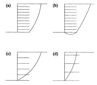
Figure 4.3 Slip Surface Types: (a) External Slip Surface; (b) Deep-Seated Slip Surface; (c) Compound Slip Surface; (d) Internal Slip Surface.


Figure 4.4. Diagram. Definition of Vertical Sections A, B, and C along which Stress and Displacement Distributions Were Investigated. This is a diagram of the components of foundation, modular blocks, reinforced soil, retained soil (backfill) and reinforcement layers as described earlier. Three thin lines representing vertical sections that were removed to assess stress and displacement distributions are marked on the diagram. Section A is directly behind the modular block facing, section B is within the reinforced soil near the end of the reinforcement, and section C is within the backfill soil, near the end of the reinforcement.

Figure 4.4 Definition of Vertical Sections A, B, and C along which Stress and Displacement Distributions Were Investigated.


(a) Figure 4.5. Grids. State of Soil for Case 1 (S equals 0.2 meters, lowercase L equals 1.5 meters):  (A) Failure State (lowercase H equals 8.6 meters, ratio of lowercase L to lowercase H equals 0.17);  (B) Critical State (lowercase H equals 6.6 meters, ratio of lowercase L to lowercase H equals 0.23). This figure represents the model for case 1, in which S equals 0.2 meters with high strength soil and very stiff foundation. Three material states are displayed on the grids: elastic; at yield in shear or volume; and elastic, yield in past. The failure state demonstrated in grid A shows elastic foundation; an area of elastic, yield in past material throughout the half of the retained soil that is farthest from the reinforcement layers, with scattered elastic states near the bottom of the retained soil; and a thick band of material at yield in shear or volume beginning at the base of the reinforcement layer and extending up at a 60-degree angle through the retained soil. The area above and to the left of this band is scattered with bands of material at yield in shear or volume intersecting material that is elastic, yield in past. There is also a band of the yielding material against the entire boundary between the reinforcement layers and the retained soil. The critical state demonstrated in grid B shows elastic foundation; a larger area of elastic, yield in past throughout approximately five-sixths of the retained soil that is farthest from the reinforcement layers with scattered elastic states near the bottom of the retained soil; and a thin band of at yield in shear or volume beginning at the base of the reinforcement layer and extending up at a 75-degree angle through the retained soil. There is also evidence of scattered material at yield in shear or volume at the base of the reinforcement layers, and a thin band of this material moving up the boundary between the reinforcement layers and the retained soil.


(b) Figure 4.5. Grids. State of Soil for Case 1 (S equals 0.2 meters, lowercase L equals 1.5 meters):  (A) Failure State (lowercase H equals 8.6 meters, ratio of lowercase L to lowercase H equals 0.17);  (B) Critical State (lowercase H equals 6.6 meters, ratio of lowercase L to lowercase H equals 0.23). This figure represents the model for case 1, in which S equals 0.2 meters with high strength soil and very stiff foundation. Three material states are displayed on the grids: elastic; at yield in shear or volume; and elastic, yield in past. The failure state demonstrated in grid A shows elastic foundation; an area of elastic, yield in past material throughout the half of the retained soil that is farthest from the reinforcement layers, with scattered elastic states near the bottom of the retained soil; and a thick band of material at yield in shear or volume beginning at the base of the reinforcement layer and extending up at a 60-degree angle through the retained soil. The area above and to the left of this band is scattered with bands of material at yield in shear or volume intersecting material that is elastic, yield in past. There is also a band of the yielding material against the entire boundary between the reinforcement layers and the retained soil. The critical state demonstrated in grid B shows elastic foundation; a larger area of elastic, yield in past throughout approximately five-sixths of the retained soil that is farthest from the reinforcement layers with scattered elastic states near the bottom of the retained soil; and a thin band of at yield in shear or volume beginning at the base of the reinforcement layer and extending up at a 75-degree angle through the retained soil. There is also evidence of scattered material at yield in shear or volume at the base of the reinforcement layers, and a thin band of this material moving up the boundary between the reinforcement layers and the retained soil.


LEGEND: State of Material
Elastic Pink Color - Represents Elastic State of Material At Yield in Shear or Volume Red Color - Represents At Yield in Shear or Volume State of Material Elastic, Yield in Past Purple Color - Represents Elastic, Yield in Past State of Material

Figure 4.5 State of Soil for Case 1 (s=0.2 m, l=1.5 m): (a) Failure State (h=8.6 m, l/h=0.17); (b) Critical State (h=6.6 m, l/h=0.23).


(a) Figure 4.6. Grids. Displacement Vectors for Case 1 (S equals 0.2 meters, lowercase L equals 1.5 meters):  (A) Failure State (lowercase H equals 8.6 meters, ratio of lowercase L to lowercase H equals 0.17);  (B) Critical State (lowercase H equals 6.6 meters, ratio of lowercase L to lowercase H equals 0.23). The figure shows the numerical grid and the displacement vectors at failure and critical state. The definition of the failure and critical state is given in the text.


(b) Figure 4.6. Grids. Displacement Vectors for Case 1 (S equals 0.2 meters, lowercase L equals 1.5 meters):  (A) Failure State (lowercase H equals 8.6 meters, ratio of lowercase L to lowercase H equals 0.17);  (B) Critical State (lowercase H equals 6.6 meters, ratio of lowercase L to lowercase H equals 0.23). The figure shows the numerical grid and the displacement vectors at failure and critical state. The definition of the failure and critical state is given in the text.

LEGEND: Maximum Vector

  1. 0.628 m
  2. 0.043 m

Figure 4.6 Displacement Vectors for Case 1 (s=0.2 m, l=1.5 m): (a) Failure State (h=8.6 m, l/h=0.17); (b) Critical State (h=6.6 m, l/h=0.23).


(a) Figure 4.7. Grids. Distorted Grid for Case 1 (S equals 0.2 meters, lowercase L equals 1.5 meters):  (A) Failure State (lowercase H equals 8.6 meters, ratio of lowercase L to lowercase H equals 0.17);  (B) Critical State (lowercase H equals 6.6 meters, ratio of lowercase L to lowercase H equals 0.23). For each state the figure shows the numerical grid for the model to scale and distorted (i.e., the cumulative displacements are artificially exaggerated for illustrative purposes).


(b) Figure 4.7. Grids. Distorted Grid for Case 1 (S equals 0.2 meters, lowercase L equals 1.5 meters):  (A) Failure State (lowercase H equals 8.6 meters, ratio of lowercase L to lowercase H equals 0.17);  (B) Critical State (lowercase H equals 6.6 meters, ratio of lowercase L to lowercase H equals 0.23). For each state the figure shows the numerical grid for the model to scale and distorted (i.e., the cumulative displacements are artificially exaggerated for illustrative purposes).

LEGEND: Maximum Displacement

  1. (a) 0.640 m
  2. (b) 0.044 m

Figure 4.7 Distorted Grid for Case 1 (s=0.2 m, l=1.5 m): (a) Failure State (h=8.6 m, l/h=0.17); (b) Critical State (h=6.6 m, l/h=0.23).


Figure 4.8. Graph. Cumulative Horizontal Displacements for Case 1 (S equals 0.2 meters, lowercase L equals 1.5 meters):  (A) Failure State (lowercase H equals 8.6 meters, ratio of lowercase L to lowercase H equals 0.17); (B) Critical State (lowercase H equals 6.6 meters, ratio of lowercase L to lowercase H equals 0.23). This figure charts failure and critical states for sections A and B for case 1. Horizontal displacement from 90 to 0 centimeters is measured on the X-axis, and elevation from 0 to 8.8 meters is measured on the Y-axis. The critical states for both sections A and B follow the same path, beginning at coordinates 0,0, increasing gradually in displacement and elevation to a high at coordinates 3, 3.6, and decreasing back to 0 centimeters horizontal displacement at an elevation of 6.6 meters. Failure states for both sections A and B also chart a similar path, beginning at coordinates 1, 0.2, increasing gradually in displacement and elevation to a high at coordinates 59, 7.2, and decreasing sharply in horizontal displacement to end at coordinates 22, 8.6.

Figure 4.8 Cumulative Horizontal Displacements for Case 1 (s=0.2 m, l=1.5 m): (a) Failure State (h=8.6 m, l/h=0.17); (b) Critical State (h=6.6 m, l/h=0.23).


(a) Figure 4.9. Drawings. Axial Force Distribution in Reinforcement for Case 1  (S equals 0.2 meters, lowercase L equals 1.5 meters):  (A) Failure State (lowercase H equals 8.6 meters, ratio of lowercase L to lowercase H equals 0.17); (B) Critical State (lowercase H equals 6.6 meters, ratio of lowercase L to lowercase H equals 0.23). This figure shows the distribution of the axial force along each reinforcement layer present at failure and critical state.


(b) Figure 4.9. Drawings. Axial Force Distribution in Reinforcement for Case 1  (S equals 0.2 meters, lowercase L equals 1.5 meters):  (A) Failure State (lowercase H equals 8.6 meters, ratio of lowercase L to lowercase H equals 0.17); (B) Critical State (lowercase H equals 6.6 meters, ratio of lowercase L to lowercase H equals 0.23). This figure shows the distribution of the axial force along each reinforcement layer present at failure and critical state.

Figure 4.9 Axial Force Distribution in Reinforcement for Case 1 (s=0.2 m, l=1.5 m): (a) Failure State (h=8.6 m, l/h=0.17); (b) Critical State (h=6.6 m, l/h=0.23).


(a) Figure 4.10. Grids. State of Soil for Case 1 (S equals 0.4 meters, lowercase L equals 1.5 meters):  (A) Failure State (lowercase H equals 8.2 meters, ratio of lowercase L to lowercase H equals 0.18); (B) Critical State (lowercase H equals 6.0 meters, ratio of lowercase L to lowercase H equals 0.25). This figure represents the model for case 1, in which S equals 0.4 meters with high strength soil and very stiff foundation. Three material states are displayed on the grids: elastic; at yield in shear or volume; and elastic, yield in past. The failure state demonstrated in grid A shows elastic foundation; an area of elastic, yield in past throughout the half of the retained soil that is farthest from the reinforcement layers, with scattered elastic states near the bottom of the retained soil; and a thick band of at yield in shear or volume beginning at the base of the reinforcement layer and extending up at a 65-degree angle through the retained soil. The area above and to the left of this band is scattered with bands of material at yield in shear or volume intersecting material that is elastic, yield in past. There is also a band of the yielding material against the entire boundary between the reinforcement layers and the retained soil. The critical state demonstrated in grid B shows elastic foundation; a larger area of elastic, yield in past throughout approximately five-sixths of the retained soil that is farthest from the reinforcement layers, with scattered elastic states near the bottom of the retained soil; and a thin band of at yield in shear or volume beginning at the third reinforcement layer and extending up at a 75-degree angle through the retained soil. There is also evidence of scattered material at yield in shear or volume at the base of the reinforcement layers, and a thin band of this material moving up the boundary between the reinforcement layers and the retained soil.


(b) Figure 4.10. Grids. State of Soil for Case 1 (S equals 0.4 meters, lowercase L equals 1.5 meters):  (A) Failure State (lowercase H equals 8.2 meters, ratio of lowercase L to lowercase H equals 0.18); (B) Critical State (lowercase H equals 6.0 meters, ratio of lowercase L to lowercase H equals 0.25). This figure represents the model for case 1, in which S equals 0.4 meters with high strength soil and very stiff foundation. Three material states are displayed on the grids: elastic; at yield in shear or volume; and elastic, yield in past. The failure state demonstrated in grid A shows elastic foundation; an area of elastic, yield in past throughout the half of the retained soil that is farthest from the reinforcement layers, with scattered elastic states near the bottom of the retained soil; and a thick band of at yield in shear or volume beginning at the base of the reinforcement layer and extending up at a 65-degree angle through the retained soil. The area above and to the left of this band is scattered with bands of material at yield in shear or volume intersecting material that is elastic, yield in past. There is also a band of the yielding material against the entire boundary between the reinforcement layers and the retained soil. The critical state demonstrated in grid B shows elastic foundation; a larger area of elastic, yield in past throughout approximately five-sixths of the retained soil that is farthest from the reinforcement layers, with scattered elastic states near the bottom of the retained soil; and a thin band of at yield in shear or volume beginning at the third reinforcement layer and extending up at a 75-degree angle through the retained soil. There is also evidence of scattered material at yield in shear or volume at the base of the reinforcement layers, and a thin band of this material moving up the boundary between the reinforcement layers and the retained soil.


LEGEND: State of Material
Elastic Pink Color - Represents Elastic State of Material At Yield in Shear or Volume Red Color - Represents At Yield in Shear or Volume State of Material Elastic, Yield in Past Purple Color - Represents Elastic, Yield in Past State of Material

Figure 4.10 State of Soil for Case 1 (s=0.4 m, l=1.5 m): (a) Failure State (h=8.2 m, l/h=0.18); (b) Critical State (h=6.0 m, l/h=0.25).


(a) Figure 4.11. Grids. State of Soil for Case 4 (S equals 0.2 meters, lowercase L equals 1.5 meters):  (A) Failure State (lowercase H equals 7.0 meters, ratio of lowercase L to lowercase H equals 0.21); (B) Critical State (lowercase H equals 5.6 meters, ratio of lowercase L to lowercase H equals 0.27). This figure represents the model for case 4, in which S equals 0.2 meters with high strength soil and baseline foundation. Three material states are displayed on the grids: elastic; at yield in shear or volume; and elastic, yield in past. The failure state demonstrated in grid A shows elastic foundation with a trough-like area to the left of the reinforcement that is a combination of material that is at yield in shear or volume and elastic, yield in past; a solid area of elastic, yield in past material throughout approximately seven-eighths of the retained soil that is farthest from the reinforcement layers; and two thick bands of material at yield in shear or volume beginning at the second reinforcement layer and extending up at a 70-degree angle through the retained soil. The area above and to the left of this band is scattered with bands of material at yield in shear or volume intersecting material that is elastic, yield in past. There is also a band of the yielding material against the entire boundary between the reinforcement layers and the retained soil. The critical state demonstrated in grid B shows elastic foundation with a smaller trough-like area to the right of the reinforcement that is a combination of material that is at yield in shear or volume and elastic, yield in past; a larger area of elastic, yield in past throughout approximately five-sixths of the retained soil that is farthest from the reinforcement layers, with scattered elastic states near the bottom of the retained soil; and a thin band of at yield in shear or volume beginning at the fourth reinforcement layer and extending up at a 75-degree angle through the retained soil. There is also a thin band of at yield in shear or volume moving up the boundary between the reinforcement layers and the retained soil and across the top of the retained soil.


(b) Figure 4.11. Grids. State of Soil for Case 4 (S equals 0.2 meters, lowercase L equals 1.5 meters):  (A) Failure State (lowercase H equals 7.0 meters, ratio of lowercase L to lowercase H equals 0.21); (B) Critical State (lowercase H equals 5.6 meters, ratio of lowercase L to lowercase H equals 0.27). This figure represents the model for case 4, in which S equals 0.2 meters with high strength soil and baseline foundation. Three material states are displayed on the grids: elastic; at yield in shear or volume; and elastic, yield in past. The failure state demonstrated in grid A shows elastic foundation with a trough-like area to the left of the reinforcement that is a combination of material that is at yield in shear or volume and elastic, yield in past; a solid area of elastic, yield in past material throughout approximately seven-eighths of the retained soil that is farthest from the reinforcement layers; and two thick bands of material at yield in shear or volume beginning at the second reinforcement layer and extending up at a 70-degree angle through the retained soil. The area above and to the left of this band is scattered with bands of material at yield in shear or volume intersecting material that is elastic, yield in past. There is also a band of the yielding material against the entire boundary between the reinforcement layers and the retained soil. The critical state demonstrated in grid B shows elastic foundation with a smaller trough-like area to the right of the reinforcement that is a combination of material that is at yield in shear or volume and elastic, yield in past; a larger area of elastic, yield in past throughout approximately five-sixths of the retained soil that is farthest from the reinforcement layers, with scattered elastic states near the bottom of the retained soil; and a thin band of at yield in shear or volume beginning at the fourth reinforcement layer and extending up at a 75-degree angle through the retained soil. There is also a thin band of at yield in shear or volume moving up the boundary between the reinforcement layers and the retained soil and across the top of the retained soil.


LEGEND: State of Material
Elastic Pink Color - Represents Elastic State of Material At Yield in Shear or Volume Red Color - Represents At Yield in Shear or Volume State of Material Elastic, Yield in Past Purple Color - Represents Elastic, Yield in Past State of Material

Figure 4.11 State of Soil for Case 4 (s=0.2 m, l=1.5 m): (a) Failure State (h=7.0 m, l/h=0.21); (b) Critical State (h=5.6 m, l/h=0.27).


(a) Figure 4.12. Grids. State of Soil for Case 9 (S equals 0.2 meters, lowercase L equals 1.5 meters):  (A) Failure State (lowercase H equals 8.2 meters, ratio of lowercase L to lowercase H equals 0.18); (B) Critical State (lowercase H equals 6.6 meters, ratio of lowercase L to lowercase H equals 0.23). This figure represents the model for case 9. Three material states are displayed on the grids: elastic; at yield in shear or volume; and elastic, yield in past. The failure state demonstrated in grid A shows elastic foundation; an area of elastic, yield in past material throughout approximately three-quarters of the retained soil that is farthest from the reinforcement layers, with scattered elastic states near the bottom of the retained soil; and a thick band of material at yield in shear or volume beginning at the base of the reinforcement layer and extending up at a 60-degree angle through the retained soil. The area above and to the left of this band is scattered with parallel bands of material at yield in shear or volume intersecting material that is elastic, yield in past. There is also a band of the yielding material against the entire boundary between the reinforcement layers and the retained soil. The critical state demonstrated in grid B shows elastic foundation; a larger area of elastic, yield in past throughout approximately five-sixths of the retained soil that is farthest from the reinforcement layers, with scattered elastic states near the bottom of the retained soil; and a thin band of at yield in shear or volume beginning at the fifth reinforcement layer and extending up at a 70-degree angle through the retained soil. There is also evidence of minimal scattered material at yield in shear or volume at the base of the reinforcement layers.


(b) Figure 4.12. Grids. State of Soil for Case 9 (S equals 0.2 meters, lowercase L equals 1.5 meters):  (A) Failure State (lowercase H equals 8.2 meters, ratio of lowercase L to lowercase H equals 0.18); (B) Critical State (lowercase H equals 6.6 meters, ratio of lowercase L to lowercase H equals 0.23). This figure represents the model for case 9. Three material states are displayed on the grids: elastic; at yield in shear or volume; and elastic, yield in past. The failure state demonstrated in grid A shows elastic foundation; an area of elastic, yield in past material throughout approximately three-quarters of the retained soil that is farthest from the reinforcement layers, with scattered elastic states near the bottom of the retained soil; and a thick band of material at yield in shear or volume beginning at the base of the reinforcement layer and extending up at a 60-degree angle through the retained soil. The area above and to the left of this band is scattered with parallel bands of material at yield in shear or volume intersecting material that is elastic, yield in past. There is also a band of the yielding material against the entire boundary between the reinforcement layers and the retained soil. The critical state demonstrated in grid B shows elastic foundation; a larger area of elastic, yield in past throughout approximately five-sixths of the retained soil that is farthest from the reinforcement layers, with scattered elastic states near the bottom of the retained soil; and a thin band of at yield in shear or volume beginning at the fifth reinforcement layer and extending up at a 70-degree angle through the retained soil. There is also evidence of minimal scattered material at yield in shear or volume at the base of the reinforcement layers.


LEGEND: State of Material
Elastic Pink Color - Represents Elastic State of Material At Yield in Shear or Volume Red Color - Represents At Yield in Shear or Volume State of Material Elastic, Yield in Past Purple Color - Represents Elastic, Yield in Past State of Material

Figure 4.12 State of Soil for Case 9 (s=0.2 m, l=1.5 m): (a) Failure State (h=8.2 m, l/h=0.18); (b) Critical State (h=6.6 m, l/h=0.23).


(a) Figure 4.13. Grids. State of Soil for Case 11 (S equals 0.2 meters, lowercase L equals 1.5 meters):  (A) Failure State (lowercase H equals 7.2 meters, ratio of lowercase L to lowercase H equals 0.21); (B) Critical State (lowercase H equals 6.0 meters, ratio of lowercase L to lowercase H equals 0.25). This figure represents the model for case 11. Three material states are displayed on the grids: elastic; at yield in shear or volume; and elastic, yield in past. The failure state demonstrated in grid A shows elastic foundation; an area of elastic, yield in past material throughout the half of the retained soil that is farthest from the reinforcement layers, with scattered elastic states near the bottom of the retained soil; and a thin band of material at yield in shear or volume beginning at the base of the reinforcement layer and extending up at a 65-degree angle through the retained soil. The area above and to the left of this band is scattered with bands of material at yield in shear or volume intersecting material that is elastic, yield in past. There are also thin strands of this at yield material extending from the base of the reinforcement layers through approximately the thirteenth layer. In addition, there is a band of the yielding material against the entire boundary between the reinforcement layers and the retained soil. The critical state demonstrated in grid B shows elastic foundation; a large area of elastic, yield in past throughout approximately seven-eighths of the retained soil that is farthest from the reinforcement layers, with scattered elastic states near the bottom of the retained soil; and a thin band of at yield in shear or volume beginning at the sixth reinforcement layer and extending up at a 65-degree angle through the retained soil. There is also evidence of scattered material at yield in shear or volume at the base of the reinforcement layers, and a thin band of this material moving up the boundary between the reinforcement layers and the retained soil. There is a thin band of at yield in shear or volume moving across the top of the retained soil.


(b) Figure 4.13. Grids. State of Soil for Case 11 (S equals 0.2 meters, lowercase L equals 1.5 meters):  (A) Failure State (lowercase H equals 7.2 meters, ratio of lowercase L to lowercase H equals 0.21); (B) Critical State (lowercase H equals 6.0 meters, ratio of lowercase L to lowercase H equals 0.25). This figure represents the model for case 11. Three material states are displayed on the grids: elastic; at yield in shear or volume; and elastic, yield in past. The failure state demonstrated in grid A shows elastic foundation; an area of elastic, yield in past material throughout the half of the retained soil that is farthest from the reinforcement layers, with scattered elastic states near the bottom of the retained soil; and a thin band of material at yield in shear or volume beginning at the base of the reinforcement layer and extending up at a 65-degree angle through the retained soil. The area above and to the left of this band is scattered with bands of material at yield in shear or volume intersecting material that is elastic, yield in past. There are also thin strands of this at yield material extending from the base of the reinforcement layers through approximately the thirteenth layer. In addition, there is a band of the yielding material against the entire boundary between the reinforcement layers and the retained soil. The critical state demonstrated in grid B shows elastic foundation; a large area of elastic, yield in past throughout approximately seven-eighths of the retained soil that is farthest from the reinforcement layers, with scattered elastic states near the bottom of the retained soil; and a thin band of at yield in shear or volume beginning at the sixth reinforcement layer and extending up at a 65-degree angle through the retained soil. There is also evidence of scattered material at yield in shear or volume at the base of the reinforcement layers, and a thin band of this material moving up the boundary between the reinforcement layers and the retained soil. There is a thin band of at yield in shear or volume moving across the top of the retained soil.


LEGEND: State of Material
Elastic Pink Color - Represents Elastic State of Material At Yield in Shear or Volume Red Color - Represents At Yield in Shear or Volume State of Material Elastic, Yield in Past Purple Color - Represents Elastic, Yield in Past State of Material

Figure 4.13 State of Soil for Case 11 (s=0.2 m, l=1.5 m): (a) Failure State (h=7.2 m, l/h=0.21); (b) Critical State (h=6.0 m, l/h=0.25).


(a) Figure 4.14. Grids. State of Soil for Case 12 (S equals 0.2 meters, lowercase L equals 1.5 meters):  (A) Failure State (lowercase H equals 9.4 meters, ratio of lowercase L to lowercase H equals 0.16); (B) Critical State (lowercase H equals 6.6 meters, ratio of lowercase L to lowercase H equals 0.23). This figure represents the model for case 12, in which S equals 0.2 meters with high strength soil and very stiff foundation. Three material states are displayed on the grids: elastic; at yield in shear or volume; and elastic, yield in past. The failure state demonstrated in grid A shows elastic foundation; an area of elastic, yield in past material throughout the half of the retained soil that is farthest from the reinforcement layers, with scattered elastic states near the bottom of the retained soil; and seven to eight thick bands of material at yield in shear or volume, one of which begins at the base of the reinforcement layer and extends up at a 60-degree angle through the retained soil, but most of the bands extend from this first band in the opposite direction, back toward the reinforcement layers at approximately a 75-degree angle. There is also a band of the yielding material against the entire boundary between the reinforcement layers and the retained soil. The critical state demonstrated in grid B shows elastic foundation; a larger area of elastic, yield in past throughout approximately five-sixths of the retained soil that is farthest from the reinforcement layers, with scattered elastic states near the bottom of the retained soil; and a thin band of at yield in shear or volume beginning at the fourth reinforcement layer and extending up at a 75-degree angle through the retained soil. There is also evidence of scattered material at yield in shear or volume at the base of the reinforcement layers, and a thin band of this material moving up the boundary between the reinforcement layers and the retained soil.


(b) Figure 4.14. Grids. State of Soil for Case 12 (S equals 0.2 meters, lowercase L equals 1.5 meters):  (A) Failure State (lowercase H equals 9.4 meters, ratio of lowercase L to lowercase H equals 0.16); (B) Critical State (lowercase H equals 6.6 meters, ratio of lowercase L to lowercase H equals 0.23). This figure represents the model for case 12, in which S equals 0.2 meters with high strength soil and very stiff foundation. Three material states are displayed on the grids: elastic; at yield in shear or volume; and elastic, yield in past. The failure state demonstrated in grid A shows elastic foundation; an area of elastic, yield in past material throughout the half of the retained soil that is farthest from the reinforcement layers, with scattered elastic states near the bottom of the retained soil; and seven to eight thick bands of material at yield in shear or volume, one of which begins at the base of the reinforcement layer and extends up at a 60-degree angle through the retained soil, but most of the bands extend from this first band in the opposite direction, back toward the reinforcement layers at approximately a 75-degree angle. There is also a band of the yielding material against the entire boundary between the reinforcement layers and the retained soil. The critical state demonstrated in grid B shows elastic foundation; a larger area of elastic, yield in past throughout approximately five-sixths of the retained soil that is farthest from the reinforcement layers, with scattered elastic states near the bottom of the retained soil; and a thin band of at yield in shear or volume beginning at the fourth reinforcement layer and extending up at a 75-degree angle through the retained soil. There is also evidence of scattered material at yield in shear or volume at the base of the reinforcement layers, and a thin band of this material moving up the boundary between the reinforcement layers and the retained soil.


LEGEND: State of Material
Elastic Pink Color - Represents Elastic State of Material At Yield in Shear or Volume Red Color - Represents At Yield in Shear or Volume State of Material Elastic, Yield in Past Purple Color - Represents Elastic, Yield in Past State of Material

Figure 4.14 State of Soil for Case 12 (s=0.2 m, l=1.5 m): (a) Failure State (h=9.4 m, l/h=0.16); (b) Critical State (h=6.6 m, l/h=0.23).


(a) Figure 4.15. Grids. State of Soil for Case 10 (S equals 0.2 meters, lowercase L equals 1.5 meters):  (A) Failure State (lowercase H equals 4.4 meters, ratio of lowercase L to lowercase H equals 0.34); (B) Critical State (lowercase H equals 3.2 meters, ratio of lowercase L to lowercase H equals 0.47). This figure represents the model for case 10, in which S equals 0.2 meters with high strength reinforced soil and low strength backfill and foundation soil. Three material states are displayed on the grids: elastic; at yield in shear or volume; and elastic, yield in past. The failure state demonstrated in grid A shows an elastic, yield in past foundation; an area of elastic, yield in past material throughout most of the retained soil, with a few horizontal bands of elastic states near the reinforced soil up into the bottom half of the retained soil; and a thick band of material at yield in shear or volume beginning in the foundation to the left of the base of the reinforcement layers, dipping under the reinforcement layers, and extending up at a 65-degree angle through the retained soil. The area above and to the left of this band is scattered with bands of material at yield in shear or volume intersecting material that is elastic, yield in past. There are also square and rectangular areas of the yielding material at the far right of the grid, throughout the foundation and the retained soil. The critical state demonstrated in grid B shows elastic, yield in past foundation; an area of elastic, yield in past material throughout most of the retained soil, with a few horizontal bands of elastic states near the reinforced soil up into the bottom half of the retained soil; and several areas of material at yield in shear or volume. The first of these areas is in the foundation, to the left of the reinforcement layers. The second of these areas begins at the base of the reinforcement layer and extends up at a 75-degree angle through the retained soil, about one-tenth of the total length of the entire retained soil, and bands of the material continue across the top of the retained soil. The third area is to the far right of the grid, throughout the foundation and the retained soil.


(b) Figure 4.15. Grids. State of Soil for Case 10 (S equals 0.2 meters, lowercase L equals 1.5 meters):  (A) Failure State (lowercase H equals 4.4 meters, ratio of lowercase L to lowercase H equals 0.34); (B) Critical State (lowercase H equals 3.2 meters, ratio of lowercase L to lowercase H equals 0.47). This figure represents the model for case 10, in which S equals 0.2 meters with high strength reinforced soil and low strength backfill and foundation soil. Three material states are displayed on the grids: elastic; at yield in shear or volume; and elastic, yield in past. The failure state demonstrated in grid A shows an elastic, yield in past foundation; an area of elastic, yield in past material throughout most of the retained soil, with a few horizontal bands of elastic states near the reinforced soil up into the bottom half of the retained soil; and a thick band of material at yield in shear or volume beginning in the foundation to the left of the base of the reinforcement layers, dipping under the reinforcement layers, and extending up at a 65-degree angle through the retained soil. The area above and to the left of this band is scattered with bands of material at yield in shear or volume intersecting material that is elastic, yield in past. There are also square and rectangular areas of the yielding material at the far right of the grid, throughout the foundation and the retained soil. The critical state demonstrated in grid B shows elastic, yield in past foundation; an area of elastic, yield in past material throughout most of the retained soil, with a few horizontal bands of elastic states near the reinforced soil up into the bottom half of the retained soil; and several areas of material at yield in shear or volume. The first of these areas is in the foundation, to the left of the reinforcement layers. The second of these areas begins at the base of the reinforcement layer and extends up at a 75-degree angle through the retained soil, about one-tenth of the total length of the entire retained soil, and bands of the material continue across the top of the retained soil. The third area is to the far right of the grid, throughout the foundation and the retained soil.


LEGEND: State of Material
Elastic Pink Color - Represents Elastic State of Material At Yield in Shear or Volume Red Color - Represents At Yield in Shear or Volume State of Material Elastic, Yield in Past Purple Color - Represents Elastic, Yield in Past State of Material

Figure 4.15 State of Soil for Case 10 (s=0.2 m, l=1.5 m): (a) Failure State (h=4.4 m, l/h=0.34); (b) Critical State (h=3.2 m, l/h=0.47).


(a) Figure 4.16. Grids. Displacement Vectors for Case 10 (S equals 0.2 meters, lowercase L equals 1.5 meters):  (A) Failure State (lowercase H equals 4.4 meters, ratio of lowercase L to lowercase H equals 0.34); (B) Critical State (lowercase H equals 3.2 meters, ratio of lowercase L to lowercase H equals 0.47). The figure shows the numerical grid and the displacement vectors at failure and critical state. The definition of the failure and critical state is given in the text


(b) Figure 4.16. Grids. Displacement Vectors for Case 10 (S equals 0.2 meters, lowercase L equals 1.5 meters):  (A) Failure State (lowercase H equals 4.4 meters, ratio of lowercase L to lowercase H equals 0.34); (B) Critical State (lowercase H equals 3.2 meters, ratio of lowercase L to lowercase H equals 0.47). The figure shows the numerical grid and the displacement vectors at failure and critical state. The definition of the failure and critical state is given in the text

LEGEND: Maximum Vector

  1. 0.325 m
  2. 0.036 m

Figure 4.16 Displacement Vectors for Case 10 (s=0.2 m, l=1.5 m): (a) Failure State (h=4.4 m, l/h=0.34); (b) Critical State (h=3.2 m, l/h=0.47).


(a) Figure 4.17. Grids. Distorted Grid for Case 10 (S equals 0.2 meters, lowercase L equals 1.5 meters):  (A) Failure State (lowercase H equals 4.4 meters, ratio of lowercase L to lowercase H equals 0.34); (B) Critical State (lowercase H equals 3.2 meters, ratio of lowercase L to lowercase H equals 0.47). For each state the figure shows the numerical grid for the model to scale and distorted (i.e., the cumulative displacements are artificially exaggerated for illustrative purposes).


(b) Figure 4.17. Grids. Distorted Grid for Case 10 (S equals 0.2 meters, lowercase L equals 1.5 meters):  (A) Failure State (lowercase H equals 4.4 meters, ratio of lowercase L to lowercase H equals 0.34); (B) Critical State (lowercase H equals 3.2 meters, ratio of lowercase L to lowercase H equals 0.47). For each state the figure shows the numerical grid for the model to scale and distorted (i.e., the cumulative displacements are artificially exaggerated for illustrative purposes).

LEGEND: Maximum Displacement

  1. 0.325 m
  2. 0.037 m

Figure 4.17 Distorted Grid for Case 10 (s=0.2 m, l=1.5 m): (a) Failure State (h=4.4 m, l/h=0.34); (b) Critical State (h=3.2 m, l/h=0.47).


Figure 4.18. Graph. Horizontal Displacements for Case 10 (S equals 0.2 meters, lowercase L equals 1.5 meters) at Failure State (lowercase H equals 4.4 meters, ratio of lowercase L to lowercase H equals 0.34) and Critical State (lowercase H equals 3.2 meters, ratio of lowercase L to lowercase H equals 0.47). This figure charts failure and critical states for sections A and B for case 10. Horizontal displacement from 40 to 0 centimeters is measured on the X-axis, and elevation from 0 to 4.4 meters is measured on the Y-axis. The critical states for both sections A and B follow the same path, beginning at coordinates 2, 0.1, increasing gradually in displacement and elevation to a high at coordinates 3, 1.4, and decreasing back to 0 centimeters horizontal displacement at an elevation of 3.2 meters. Failure states for both sections A and B also chart a similar path. Section A begins at coordinates 15, 0.1, and section B begins at coordinates 11, 0.1. The sections converge at coordinates 15, 0.4, and increase gradually in displacement and elevation to a high at coordinates 30, 3.6, then decrease sharply in horizontal displacement to end at coordinates 15, 4.4.

Figure 4.18. Horizontal Displacements for Case 10 (s=0.2 m, l=1.5 m) at Failure State (h=4.4 m, l/h=0.34) and Critical State (h=3.2 m, l/h=0.47).


(a) Figure 4.19. Drawings. Axial Force Distribution in Reinforcement for Case 10 (S equals 0.2 meters, lowercase L equals 1.5 meters):  (A) Failure State (lowercase H equals 4.4 meters, ratio of lowercase L to lowercase H equals 0.34); (B) Critical State (lowercase H equals 3.2 meters, ratio of lowercase L to lowercase H equals 0.47). This figure shows the distribution of the axial force along each reinforcement layer present at failure and critical state.


(b) Figure 4.19. Drawings. Axial Force Distribution in Reinforcement for Case 10 (S equals 0.2 meters, lowercase L equals 1.5 meters):  (A) Failure State (lowercase H equals 4.4 meters, ratio of lowercase L to lowercase H equals 0.34); (B) Critical State (lowercase H equals 3.2 meters, ratio of lowercase L to lowercase H equals 0.47). This figure shows the distribution of the axial force along each reinforcement layer present at failure and critical state.

Figure 4.19 Axial Force Distribution in Reinforcement for Case 10 (s=0.2 m, l=1.5 m): (a) Failure State (h=4.4 m, l/h=0.34); (b) Critical State (h=3.2 m, l/h=0.47).


(a) Figure 4.20. Grids. State of Soil for Case 5 (S equals 0.2 meters, lowercase L equals 1.5 meters):  (A) Failure State (lowercase H equals 5.4 meters, ratio of lowercase L to lowercase H equals 0.28); (B) Critical State (lowercase H equals 4.2 meters, ratio of lowercase L to lowercase H equals 0.36). This figure represents the model for case 5, in which S equals 0.2 meters with low strength soil and baseline foundation. Three material states are displayed on the grids: elastic; at yield in shear or volume; and elastic, yield in past. The failure state demonstrated in grid A shows elastic foundation with a trough-like area to the left of the reinforcement that extends approximately halfway through the foundation; this area is a combination of material that is at yield in shear or volume and material that is elastic, yield in past; an area of elastic, yield in past material throughout five-sixths of the retained soil that is farthest from the reinforcement layers; and a thick band of material at yield in shear or volume that begins at the trough, continues under the reinforcement layer, and extends up at a 65-degree angle through the retained soil. There is a band of material that is elastic, yield in past above and to the left of this band, and above this band is a solid area of material at yield in shear or volume that abuts the reinforcement layers. There is also a band of the yielding material against the entire boundary between the reinforcement layers and the retained soil. The critical state demonstrated in grid B shows elastic foundation with a trough-like area to the left of the reinforcement that extends approximately one-fourth of the way down through the foundation; a larger area of elastic, yield in past throughout approximately five-sixths of the retained soil that is farthest from the reinforcement layers; and a relatively solid area of material at yield in shear or volume that extends up at a 65-degree angle through the retained soil beginning at the base of the reinforcement layer and includes the area between this angle and the reinforcement layer. There is also evidence of scattered material at yield in shear or volume at the base of the reinforcement layers.


(b) Figure 4.20. Grids. State of Soil for Case 5 (S equals 0.2 meters, lowercase L equals 1.5 meters):  (A) Failure State (lowercase H equals 5.4 meters, ratio of lowercase L to lowercase H equals 0.28); (B) Critical State (lowercase H equals 4.2 meters, ratio of lowercase L to lowercase H equals 0.36). This figure represents the model for case 5, in which S equals 0.2 meters with low strength soil and baseline foundation. Three material states are displayed on the grids: elastic; at yield in shear or volume; and elastic, yield in past. The failure state demonstrated in grid A shows elastic foundation with a trough-like area to the left of the reinforcement that extends approximately halfway through the foundation; this area is a combination of material that is at yield in shear or volume and material that is elastic, yield in past; an area of elastic, yield in past material throughout five-sixths of the retained soil that is farthest from the reinforcement layers; and a thick band of material at yield in shear or volume that begins at the trough, continues under the reinforcement layer, and extends up at a 65-degree angle through the retained soil. There is a band of material that is elastic, yield in past above and to the left of this band, and above this band is a solid area of material at yield in shear or volume that abuts the reinforcement layers. There is also a band of the yielding material against the entire boundary between the reinforcement layers and the retained soil. The critical state demonstrated in grid B shows elastic foundation with a trough-like area to the left of the reinforcement that extends approximately one-fourth of the way down through the foundation; a larger area of elastic, yield in past throughout approximately five-sixths of the retained soil that is farthest from the reinforcement layers; and a relatively solid area of material at yield in shear or volume that extends up at a 65-degree angle through the retained soil beginning at the base of the reinforcement layer and includes the area between this angle and the reinforcement layer. There is also evidence of scattered material at yield in shear or volume at the base of the reinforcement layers.


LEGEND: State of Material
Elastic Pink Color - Represents Elastic State of Material At Yield in Shear or Volume Red Color - Represents At Yield in Shear or Volume State of Material Elastic, Yield in Past Purple Color - Represents Elastic, Yield in Past State of Material

Figure 4.20 State of Soil for Case 5 (s=0.2 m, l=1.5 m): (a) Failure State (h=5.4 m, l/h=0.28); (b) Critical State (h=4.2 m, l/h=0.36).


(a) Figure 4.21. Grids. State of Soil for Case 8-1 (S equals 0.4 meters, lowercase L equals 1.5 meters):  (A) Failure State (lowercase H equals 8.0 meters, ratio of lowercase L to lowercase H equals 0.19); (B) Critical State (lowercase H equals 5.0 meters, ratio of lowercase L to lowercase H equals 0.3). This figure represents the model for case 8-1, in which S equals 0.4 meters with high strength soil and very stiff foundation. Three material states are displayed on the grids: elastic; at yield in shear or volume; and elastic, yield in past. The failure state demonstrated in grid A shows elastic foundation; an area of elastic, yield in past material throughout one-half of the retained soil that is farthest from the reinforcement layers, with thin bands of elastic material scattered in the bottom half of the retained soil; and an area of material at yield in shear or volume that begins at the base of the reinforcement layers and extends up at a 60-degree angle through the retained soil. The area above and to the left of this boundary is scattered with material that is elastic, yield in past and material at yield in shear or volume. The bottom six reinforcement layers are bulging to the left. The critical state demonstrated in grid B shows elastic foundation; a larger area of elastic, yield in past throughout approximately seven-eighths of the retained soil that is farthest from the reinforcement layers, with thin bands of elastic material scattered in the bottom half of the retained soil; and a relatively solid area of material at yield in shear or volume that extends up at a 65-degree angle through the retained soil beginning at the base of the reinforcement layer and includes the area between this angle and the abutment wall.


(b) Figure 4.21. Grids. State of Soil for Case 8-1 (S equals 0.4 meters, lowercase L equals 1.5 meters):  (A) Failure State (lowercase H equals 8.0 meters, ratio of lowercase L to lowercase H equals 0.19); (B) Critical State (lowercase H equals 5.0 meters, ratio of lowercase L to lowercase H equals 0.3). This figure represents the model for case 8-1, in which S equals 0.4 meters with high strength soil and very stiff foundation. Three material states are displayed on the grids: elastic; at yield in shear or volume; and elastic, yield in past. The failure state demonstrated in grid A shows elastic foundation; an area of elastic, yield in past material throughout one-half of the retained soil that is farthest from the reinforcement layers, with thin bands of elastic material scattered in the bottom half of the retained soil; and an area of material at yield in shear or volume that begins at the base of the reinforcement layers and extends up at a 60-degree angle through the retained soil. The area above and to the left of this boundary is scattered with material that is elastic, yield in past and material at yield in shear or volume. The bottom six reinforcement layers are bulging to the left. The critical state demonstrated in grid B shows elastic foundation; a larger area of elastic, yield in past throughout approximately seven-eighths of the retained soil that is farthest from the reinforcement layers, with thin bands of elastic material scattered in the bottom half of the retained soil; and a relatively solid area of material at yield in shear or volume that extends up at a 65-degree angle through the retained soil beginning at the base of the reinforcement layer and includes the area between this angle and the abutment wall.


LEGEND: State of Material
Elastic Pink Color - Represents Elastic State of Material At Yield in Shear or Volume Red Color - Represents At Yield in Shear or Volume State of Material Elastic, Yield in Past Purple Color - Represents Elastic, Yield in Past State of Material

Figure 4.21 State of Soil for Case 8–1 (s=0.4 m, l=1.5 m): (a) Failure State (h=8.0 m, l/h=0.19); (b) Critical State (h=5.0 m, l/h=0.3).


(a) Figure 4.22. Grids. Displacement Vectors for Case 8-1 (S equals 0.4 meters, lowercase L equals 1.5 meters):  (A) Failure State (lowercase H equals 8.0 meters, ratio of lowercase L to lowercase H equals 0.19); (B) Critical State (lowercase H equals 5.0 meters, ratio of lowercase L to lowercase H equals 0.30). The figure shows the numerical grid and the displacement vectors at failure and critical state. The definition of the failure and critical state is given in the text


(b) Figure 4.22. Grids. Displacement Vectors for Case 8-1 (S equals 0.4 meters, lowercase L equals 1.5 meters):  (A) Failure State (lowercase H equals 8.0 meters, ratio of lowercase L to lowercase H equals 0.19); (B) Critical State (lowercase H equals 5.0 meters, ratio of lowercase L to lowercase H equals 0.30). The figure shows the numerical grid and the displacement vectors at failure and critical state. The definition of the failure and critical state is given in the text

LEGEND: Maximum Vector

  1. 1.221 m
  2. 0.0704 m

Figure 4.22 Displacement Vectors for Case 8–1 (s=0.4 m, l=1.5 m): (a) Failure State (h=8.0 m, l/h=0.19); (b) Critical State (h=5.0 m, l/h=0.30).


(a) Figure 4.23. Grids. Distorted Grid for Case 8-1 (S equals 0.4 meters, lowercase L equals 1.5 meters):  (A) Failure State (lowercase H equals 8.0 meters, ratio of lowercase L to lowercase H equals 0.19); (B) Critical State (lowercase H equals 5.0 meters, ratio of lowercase L to lowercase H equals 0.30). For each state the figure shows the numerical grid for the model to scale and distorted (i.e., the cumulative displacements are artificially exaggerated for illustrative purposes).


(b) Figure 4.23. Grids. Distorted Grid for Case 8-1 (S equals 0.4 meters, lowercase L equals 1.5 meters):  (A) Failure State (lowercase H equals 8.0 meters, ratio of lowercase L to lowercase H equals 0.19); (B) Critical State (lowercase H equals 5.0 meters, ratio of lowercase L to lowercase H equals 0.30). For each state the figure shows the numerical grid for the model to scale and distorted (i.e., the cumulative displacements are artificially exaggerated for illustrative purposes).

LEGEND: Maximum Displacement

  1. 1.227 m
  2. 0.073 m

Figure 4.23 Distorted Grid for Case 8–1 (s=0.4 m, l=1.5 m): (a) Failure State (h=8.0 m, l/h=0.19); (b) Critical State (h=5.0 m, l/h=0.30).


Figure 4.24. Graph. Horizontal Displacements for Case 8-1 (S equals 0.4 meters, lowercase L equals 1.5 meters) at Failure (lowercase H equals 8.0 meters, ratio of lowercase L to lowercase H equals 0.19) and Critical State (lowercase H equals 5.0 meters, ratio of lowercase L to lowercase H equals 0.30). This figure charts failure and critical states for sections A and B for case 8-1. Horizontal displacement from 180 to 0 centimeters is measured on the X-axis, and elevation from 0 to 8 meters is measured on the Y-axis. The critical states for both sections A and B follow similar paths, with the critical state for section A at slightly higher horizontal displacements than section B at the same elevations. Their paths begin at coordinates 0, 0.1, increasing gradually in displacement and elevation to a high at coordinates 5, 2.0 for section A and 3, 2.6 for section B, then decreasing back to 0 centimeters horizontal displacement at an elevation of 5 meters for both sections. Failure states for sections A and B also chart a similar path, with section A at slightly higher horizontal displacements than section B at the same elevations. Section A begins at coordinates 0, 0.1, and section B begins at coordinates 1, 0.5. Both sections A and B increase gradually in displacement and elevation to highs at coordinates 118, 4.7, and 115, 4.7, respectively, then decrease almost as gradually in horizontal displacement to end at coordinates 20, 8.

Figure 4.24 Horizontal Displacements for Case 8–1 (s=0.4 m, l=1.5 m) at Failure (h=8.0 m, l/h=0.19) and Critical State (h=5.0 m, l/h=0.30).


(a)Figure 4.25. Drawings. Axial Force Distribution in Reinforcement for Case 8-1 (S equals 0.4 meters, lowercase L equals 1.5 meters):  (A) Failure State (lowercase H equals 8.0 meters, ratio of lowercase L to lowercase H equals 0.19); (B) Critical State (lowercase H equals 5.0 meters, ratio of lowercase L to lowercase H equals 0.30). This figure shows the distribution of the axial force along each reinforcement layer present at failure and critical state.

(b)Figure 4.25. Drawings. Axial Force Distribution in Reinforcement for Case 8-1 (S equals 0.4 meters, lowercase L equals 1.5 meters):  (A) Failure State (lowercase H equals 8.0 meters, ratio of lowercase L to lowercase H equals 0.19); (B) Critical State (lowercase H equals 5.0 meters, ratio of lowercase L to lowercase H equals 0.30). This figure shows the distribution of the axial force along each reinforcement layer present at failure and critical state.

Figure 4.25 Axial Force Distribution in Reinforcement for Case 8–1 (s=0.4 m, l=1.5 m): (a) Failure State (h=8.0 m, l/h=0.19); (b) Critical State (h=5.0 m, l/h=0.30).


(a) Figure 4.26. Grids. State of Soil for Case 2 (S equals 0.4 meters, lowercase L equals 1.5 meters):  (A) Failure State (lowercase H equals 6.0 meters, ratio of lowercase L to lowercase H equals 0.25); (B) Critical State (lowercase H equals 4.4 meters, ratio of lowercase L to lowercase H equals 0.34). This figure represents the model for case 2, in which S equals 0.4 meters with medium strength soil and very stiff foundation. Three material states are displayed on the grids: elastic; at yield in shear or volume; and elastic, yield in past. The failure state demonstrated in grid A shows elastic foundation; an area of elastic, yield in past material throughout four-fifths of the retained soil that is farthest from the reinforcement layers, with thin bands of elastic material scattered in the bottom three-fourths of the retained soil; and a triangular area of material at yield in shear or volume that begins at the third reinforcement layer, extends up at a 60-degree angle through the retained soil, and includes the area above and to the left of this line, to the right edge of the reinforcement layers. There are also thin bands of this at yield material extending from the base of the reinforcement layers through approximately the eighth layer. There are small areas of material that is elastic, yield in past within the triangle. The critical state demonstrated in grid B shows elastic foundation; an area similar in size to that of the failure state of elastic, yield in past in the retained soil that is farthest from the reinforcement layers; and a relatively solid triangular area of material at yield in shear or volume that extends up at a 60-degree angle through the retained soil beginning at the base of the reinforcement layer and includes the area between this angle and the reinforcement layer. There are small areas of material that is elastic, yield in past within the triangle. There is also evidence of scattered material at yield in shear or volume at the base of the reinforcement layers through the eighth layer.


(b) Figure 4.26. Grids. State of Soil for Case 2 (S equals 0.4 meters, lowercase L equals 1.5 meters):  (A) Failure State (lowercase H equals 6.0 meters, ratio of lowercase L to lowercase H equals 0.25); (B) Critical State (lowercase H equals 4.4 meters, ratio of lowercase L to lowercase H equals 0.34). This figure represents the model for case 2, in which S equals 0.4 meters with medium strength soil and very stiff foundation. Three material states are displayed on the grids: elastic; at yield in shear or volume; and elastic, yield in past. The failure state demonstrated in grid A shows elastic foundation; an area of elastic, yield in past material throughout four-fifths of the retained soil that is farthest from the reinforcement layers, with thin bands of elastic material scattered in the bottom three-fourths of the retained soil; and a triangular area of material at yield in shear or volume that begins at the third reinforcement layer, extends up at a 60-degree angle through the retained soil, and includes the area above and to the left of this line, to the right edge of the reinforcement layers. There are also thin bands of this at yield material extending from the base of the reinforcement layers through approximately the eighth layer. There are small areas of material that is elastic, yield in past within the triangle. The critical state demonstrated in grid B shows elastic foundation; an area similar in size to that of the failure state of elastic, yield in past in the retained soil that is farthest from the reinforcement layers; and a relatively solid triangular area of material at yield in shear or volume that extends up at a 60-degree angle through the retained soil beginning at the base of the reinforcement layer and includes the area between this angle and the reinforcement layer. There are small areas of material that is elastic, yield in past within the triangle. There is also evidence of scattered material at yield in shear or volume at the base of the reinforcement layers through the eighth layer.


LEGEND: State of Material
Elastic Pink Color - Represents Elastic State of Material At Yield in Shear or Volume Red Color - Represents At Yield in Shear or Volume State of Material Elastic, Yield in Past Purple Color - Represents Elastic, Yield in Past State of Material

Figure 4.26 State of Soil for Case 2 (s=0.4 m, l=1.5 m): (a) Failure State (h=6.0 m, l/h=0.25); (b) Critical State (h=4.4 m, l/h=0.34).


(a) Figure 4.27. Grids. State of Soil for Case 3 (S equals 0.2 meters, lowercase L equals 1.5 meters):  (A) Failure State (lowercase H equals 4.2 meters, ratio of lowercase L to lowercase H equals 0.36); (B) Critical State (lowercase H equals 4.0 meters, ratio of lowercase L to lowercase H equals 0.38). This figure represents the model for case 3. Three material states are displayed on the grids: elastic; at yield in shear or volume; and elastic, yield in past. The failure state demonstrated in grid A shows elastic foundation; an area of elastic, yield in past material throughout five-sixths of the retained soil that is farthest from the reinforcement layers; and a triangular area of material at yield in shear or volume that begins at the third reinforcement layer, extends up at a 60-degree angle through the retained soil, and includes the area above and to the left of this line, to the right edge of the reinforcement layers. There are also thin bands of this at yield material extending from the base of the reinforcement layers through approximately the fifteenth layer, including a strand next to the abutment wall. There are small areas of material that is elastic, yield in past within the triangle. The critical state demonstrated in grid B shows elastic foundation; an area similar in size to that of the failure state of elastic, yield in past in the retained soil that is farthest from the reinforcement layers; and a relatively solid triangular area of material at yield in shear or volume that extends up at a 60-degree angle through the retained soil beginning at the base of the reinforcement layer and includes the area between this angle and the reinforcement layer. There are small areas of material that is elastic, yield in past within the triangle. There are also thin bands of the at yield in shear of volume material extending from the base of the reinforcement layers through approximately the twelfth layer, including a strand next to the abutment wall.


(b) Figure 4.27. Grids. State of Soil for Case 3 (S equals 0.2 meters, lowercase L equals 1.5 meters):  (A) Failure State (lowercase H equals 4.2 meters, ratio of lowercase L to lowercase H equals 0.36); (B) Critical State (lowercase H equals 4.0 meters, ratio of lowercase L to lowercase H equals 0.38). This figure represents the model for case 3. Three material states are displayed on the grids: elastic; at yield in shear or volume; and elastic, yield in past. The failure state demonstrated in grid A shows elastic foundation; an area of elastic, yield in past material throughout five-sixths of the retained soil that is farthest from the reinforcement layers; and a triangular area of material at yield in shear or volume that begins at the third reinforcement layer, extends up at a 60-degree angle through the retained soil, and includes the area above and to the left of this line, to the right edge of the reinforcement layers. There are also thin bands of this at yield material extending from the base of the reinforcement layers through approximately the fifteenth layer, including a strand next to the abutment wall. There are small areas of material that is elastic, yield in past within the triangle. The critical state demonstrated in grid B shows elastic foundation; an area similar in size to that of the failure state of elastic, yield in past in the retained soil that is farthest from the reinforcement layers; and a relatively solid triangular area of material at yield in shear or volume that extends up at a 60-degree angle through the retained soil beginning at the base of the reinforcement layer and includes the area between this angle and the reinforcement layer. There are small areas of material that is elastic, yield in past within the triangle. There are also thin bands of the at yield in shear of volume material extending from the base of the reinforcement layers through approximately the twelfth layer, including a strand next to the abutment wall.


LEGEND: State of Material
Elastic Pink Color - Represents Elastic State of Material At Yield in Shear or Volume Red Color - Represents At Yield in Shear or Volume State of Material Elastic, Yield in Past Purple Color - Represents Elastic, Yield in Past State of Material

Figure 4.27 State of Soil for Case 3 (s=0.2 m, l=1.5 m): (a) Failure State (h=4.2 m, l/h=0.36); (b) Critical State (h=4.0 m, l/h=0.38).


(a) Figure 4.28. Grids. State of Soil for Case 7 (The spacing of the primary reinforcment layers was 0.6 m, and the spacing of the secondary reinforcement layers was 0.2 meters.):  (A) Failure State (lowercase H equals 6.0 meters, ratio of lowercase L to lowercase H equals 0.25); (B) Critical State (lowercase H equals 5.0 meters, ratio of lowercase L to lowercase H equals 0.30). This figure represents the model for case 7. Three material states are displayed on the grids: elastic; at yield in shear or volume; and elastic, yield in past. The failure state demonstrated in grid A shows elastic foundation; an area of elastic, yield in past material throughout seven-eighths of the retained soil that is farthest from the reinforcement layers, with scattered elastic states throughout two-thirds of the bottom of the retained soil; and a thick band of material at yield in shear or volume beginning at the base of the reinforcement layer and extending up at a 75-degree angle through the retained soil. The area above and to the left of this band is scattered with bands of material at yield in shear or volume intersecting material that is elastic, yield in past. There is also a band of the yield in shear or volume material against the entire boundary between the reinforcement layers and the retained soil, and horizontal bands of this material in the first seven reinforcement layers.The critical state demonstrated in grid B shows elastic foundation; a larger area of elastic, yield in past throughout approximately seven-eighths of the retained soil that is farthest from the reinforcement layers, with scattered elastic states throughout most of the retained soil; and a thin band of at yield in shear or volume material beginning at the third reinforcement layer and extending up at a 75-degree angle through the retained soil. There is also evidence of scattered material at yield in shear or volume at the base of the reinforcement layers.


(b) Figure 4.28. Grids. State of Soil for Case 7 (The spacing of the primary reinforcment layers was 0.6 m, and the spacing of the secondary reinforcement layers was 0.2 meters.):  (A) Failure State (lowercase H equals 6.0 meters, ratio of lowercase L to lowercase H equals 0.25); (B) Critical State (lowercase H equals 5.0 meters, ratio of lowercase L to lowercase H equals 0.30). This figure represents the model for case 7. Three material states are displayed on the grids: elastic; at yield in shear or volume; and elastic, yield in past. The failure state demonstrated in grid A shows elastic foundation; an area of elastic, yield in past material throughout seven-eighths of the retained soil that is farthest from the reinforcement layers, with scattered elastic states throughout two-thirds of the bottom of the retained soil; and a thick band of material at yield in shear or volume beginning at the base of the reinforcement layer and extending up at a 75-degree angle through the retained soil. The area above and to the left of this band is scattered with bands of material at yield in shear or volume intersecting material that is elastic, yield in past. There is also a band of the yield in shear or volume material against the entire boundary between the reinforcement layers and the retained soil, and horizontal bands of this material in the first seven reinforcement layers.The critical state demonstrated in grid B shows elastic foundation; a larger area of elastic, yield in past throughout approximately seven-eighths of the retained soil that is farthest from the reinforcement layers, with scattered elastic states throughout most of the retained soil; and a thin band of at yield in shear or volume material beginning at the third reinforcement layer and extending up at a 75-degree angle through the retained soil. There is also evidence of scattered material at yield in shear or volume at the base of the reinforcement layers.


LEGEND: State of Material
Elastic Pink Color - Represents Elastic State of Material At Yield in Shear or Volume Red Color - Represents At Yield in Shear or Volume State of Material Elastic, Yield in Past Purple Color - Represents Elastic, Yield in Past State of Material

Figure 4.28 State of Soil for Case 7 (s=0.6/0.2 m, l=1.5 m): (a) Failure State (h=6.0 m, l/h=0.25); (b) Critical State (h=5.0 m, l/h=0.30).


(a) Figure 4.29. Grids. State of Soil for Case 8-2 (S equals 0.4 meters, lowercase L equals 1.5 meters):  (A) Failure State (lowercase H equals 5.4 meters, ratio of lowercase L to lowercase H equals 0.28); (B) Critical State (lowercase H equals 3.2 meters, ratio of lowercase L to lowercase H equals 0.47). This figure represents the model for case 8-2, in which S equals 0.4 meters with medium strength soil and very stiff foundation. Three material states are displayed on the grids: elastic; at yield in shear or volume; and elastic, yield in past. The failure state demonstrated in grid A shows elastic foundation with a very small trough of elastic, yield in past material to the left of the reinforcement layers; an area of elastic, yield in past material throughout five-sixths of the retained soil that is farthest from the reinforcement layers, with scattered bands of elastic material states throughout the lower five-sixths of the retained soil; and a triangular area of material at yield in shear or volume that begins at the abutment wall and extends up at a 60-degree angle through the reinforcement layers and retained soil, and includes the area above and to the left of this line, to the right edge of the reinforcement layers. There is a solid triangular area of material that is elastic, yield in past within this triangle of material at yield in shear or volume. The critical state demonstrated in grid B shows elastic foundation; an area of elastic, yield in past material in the seven-eighths of the retained soil that is farthest from the reinforcement layers; and a relatively solid triangular area of material at yield in shear or volume that extends up at a 65-degree angle through the retained soil beginning at the base of the abutment wall and includes the area between this angle and the abutment wall. There are small areas of material that is elastic, yield in past within the triangle.


(b) Figure 4.29. Grids. State of Soil for Case 8-2 (S equals 0.4 meters, lowercase L equals 1.5 meters):  (A) Failure State (lowercase H equals 5.4 meters, ratio of lowercase L to lowercase H equals 0.28); (B) Critical State (lowercase H equals 3.2 meters, ratio of lowercase L to lowercase H equals 0.47). This figure represents the model for case 8-2, in which S equals 0.4 meters with medium strength soil and very stiff foundation. Three material states are displayed on the grids: elastic; at yield in shear or volume; and elastic, yield in past. The failure state demonstrated in grid A shows elastic foundation with a very small trough of elastic, yield in past material to the left of the reinforcement layers; an area of elastic, yield in past material throughout five-sixths of the retained soil that is farthest from the reinforcement layers, with scattered bands of elastic material states throughout the lower five-sixths of the retained soil; and a triangular area of material at yield in shear or volume that begins at the abutment wall and extends up at a 60-degree angle through the reinforcement layers and retained soil, and includes the area above and to the left of this line, to the right edge of the reinforcement layers. There is a solid triangular area of material that is elastic, yield in past within this triangle of material at yield in shear or volume. The critical state demonstrated in grid B shows elastic foundation; an area of elastic, yield in past material in the seven-eighths of the retained soil that is farthest from the reinforcement layers; and a relatively solid triangular area of material at yield in shear or volume that extends up at a 65-degree angle through the retained soil beginning at the base of the abutment wall and includes the area between this angle and the abutment wall. There are small areas of material that is elastic, yield in past within the triangle.


LEGEND: State of Material
Elastic Pink Color - Represents Elastic State of Material At Yield in Shear or Volume Red Color - Represents At Yield in Shear or Volume State of Material Elastic, Yield in Past Purple Color - Represents Elastic, Yield in Past State of Material

Figure 4.29 State of Soil for Case 8–2 (s=0.4 m, l=1.5 m): (a) Failure State (h=5.4 m, l/h=0.28); (b) Critical State (h=3.2 m, l/h=0.47).


(a) Figure 4.30. Grids. State of Soil for Case 8-3 (S equals 0.2 meters, lowercase L equals 1.5 meters):  (A) Failure State (lowercase H equals 5.0 meters, ratio of lowercase L to lowercase H equals 0.30); (B) Critical State (lowercase H equals 2.2 meters, ratio of lowercase L to lowercase H equals 0.68). This figure represents the model for case 8-3, in which S equals 0.2 meters with low strength soil and very stiff foundation. Three material states are displayed on the grids: elastic; at yield in shear or volume; and elastic, yield in past. The failure state demonstrated in grid A shows elastic foundation with a very small trough of elastic, yield in past material to the left of the reinforcement layers; an area of elastic, yield in past material throughout five-sixths of the retained soil that is farthest from the reinforcement layers, with a few bands of elastic material in the middle of the retained soil; and a triangular area of material at yield in shear or volume that begins at the reinforcement layers and extends up at a 55-degree angle through the reinforcement layers and retained soil, and includes the area above and to the left of this line, to the right edge of the reinforcement layers. There are a few scattered areas of material that is elastic, yield in past within this triangle of material at yield in shear or volume. Horizontal bands of material at yield in shear or volume cross the lowest five reinforcement layers. The critical state demonstrated in grid B shows elastic foundation; an area of elastic, yield in past material in the nine-tenths of the retained soil that is farthest from the reinforcement layers; and a relatively solid triangular area of material at yield in shear or volume that extends up at a 60-degree angle through the retained soil beginning at the base of the abutment wall and includes the area between this angle and the abutment wall. There are small areas of material that is elastic, yield in past within the triangle.


(b) Figure 4.30. Grids. State of Soil for Case 8-3 (S equals 0.2 meters, lowercase L equals 1.5 meters):  (A) Failure State (lowercase H equals 5.0 meters, ratio of lowercase L to lowercase H equals 0.30); (B) Critical State (lowercase H equals 2.2 meters, ratio of lowercase L to lowercase H equals 0.68). This figure represents the model for case 8-3, in which S equals 0.2 meters with low strength soil and very stiff foundation. Three material states are displayed on the grids: elastic; at yield in shear or volume; and elastic, yield in past. The failure state demonstrated in grid A shows elastic foundation with a very small trough of elastic, yield in past material to the left of the reinforcement layers; an area of elastic, yield in past material throughout five-sixths of the retained soil that is farthest from the reinforcement layers, with a few bands of elastic material in the middle of the retained soil; and a triangular area of material at yield in shear or volume that begins at the reinforcement layers and extends up at a 55-degree angle through the reinforcement layers and retained soil, and includes the area above and to the left of this line, to the right edge of the reinforcement layers. There are a few scattered areas of material that is elastic, yield in past within this triangle of material at yield in shear or volume. Horizontal bands of material at yield in shear or volume cross the lowest five reinforcement layers. The critical state demonstrated in grid B shows elastic foundation; an area of elastic, yield in past material in the nine-tenths of the retained soil that is farthest from the reinforcement layers; and a relatively solid triangular area of material at yield in shear or volume that extends up at a 60-degree angle through the retained soil beginning at the base of the abutment wall and includes the area between this angle and the abutment wall. There are small areas of material that is elastic, yield in past within the triangle.


LEGEND: State of Material
Elastic Pink Color - Represents Elastic State of Material At Yield in Shear or Volume Red Color - Represents At Yield in Shear or Volume State of Material Elastic, Yield in Past Purple Color - Represents Elastic, Yield in Past State of Material

Figure 4.30 State of Soil for Case 8–3 (s=0.2 m, l=1.5 m): (a) Failure State (h=5.0 m, l/h=0.30); (b) Critical State (h=2.2 m, l/h=0.68).


(a) Figure 4.31. Grids. State of Soil for Case 12 (S equals 0.6 meters, lowercase L equals 1.5 meters):  (A) Failure State (lowercase H equals 6.0 meters, ratio of lowercase L to lowercase H equals 0.25); (B) Critical State (lowercase H equals 4.6 meters, ratio of lowercase L to lowercase H equals 0.33). This figure represents the model for case 12, in which S equals 0.6 meters with high strength soil and very stiff foundation. Three material states are displayed on the grids: elastic; at yield in shear or volume; and elastic, yield in past. The failure state demonstrated in grid A shows elastic foundation; an area of elastic, yield in past material throughout the most of the retained soil that is farthest from the reinforcement layers, with scattered elastic states near the bottom of the retained soil; and a thick band of material at yield in shear or volume beginning at the base of the abutment wall and extending up at a 70-degree angle through the retained soil. The area above and to the left of this band is primarily material that is elastic, yield in past. There is also a band of the at yield in shear or volume material against the entire boundary between the reinforcement layers and the retained soil. The critical state demonstrated in grid B is almost identical to grid A it shows elastic foundation; an area of elastic, yield in past material throughout the most of the retained soil that is farthest from the reinforcement layers, with scattered elastic states near the bottom of the retained soil; and a thick band of material at yield in shear or volume beginning at the base of the abutment wall and extending up at a 70-degree angle through the retained soil. The area above and to the left of this band is primarily material that is elastic, yield in past. There is also a band of the at yield in shear or volume material against the entire boundary between the reinforcement layers and the retained soil.


(b) Figure 4.31. Grids. State of Soil for Case 12 (S equals 0.6 meters, lowercase L equals 1.5 meters):  (A) Failure State (lowercase H equals 6.0 meters, ratio of lowercase L to lowercase H equals 0.25); (B) Critical State (lowercase H equals 4.6 meters, ratio of lowercase L to lowercase H equals 0.33). This figure represents the model for case 12, in which S equals 0.6 meters with high strength soil and very stiff foundation. Three material states are displayed on the grids: elastic; at yield in shear or volume; and elastic, yield in past. The failure state demonstrated in grid A shows elastic foundation; an area of elastic, yield in past material throughout the most of the retained soil that is farthest from the reinforcement layers, with scattered elastic states near the bottom of the retained soil; and a thick band of material at yield in shear or volume beginning at the base of the abutment wall and extending up at a 70-degree angle through the retained soil. The area above and to the left of this band is primarily material that is elastic, yield in past. There is also a band of the at yield in shear or volume material against the entire boundary between the reinforcement layers and the retained soil. The critical state demonstrated in grid B is almost identical to grid A it shows elastic foundation; an area of elastic, yield in past material throughout the most of the retained soil that is farthest from the reinforcement layers, with scattered elastic states near the bottom of the retained soil; and a thick band of material at yield in shear or volume beginning at the base of the abutment wall and extending up at a 70-degree angle through the retained soil. The area above and to the left of this band is primarily material that is elastic, yield in past. There is also a band of the at yield in shear or volume material against the entire boundary between the reinforcement layers and the retained soil.


LEGEND: State of Material
Elastic Pink Color - Represents Elastic State of Material At Yield in Shear or Volume Red Color - Represents At Yield in Shear or Volume State of Material Elastic, Yield in Past Purple Color - Represents Elastic, Yield in Past State of Material

Figure 4.31 State of Soil for Case 12 (s=0.6 m, l=1.5 m): (a) Failure State (h=6.0 m, l/h=0.25); (b) Critical State (h=4.6 m, l/h=0.33).


(a) Figure 4.32. Grids. State of Soil for Case 2 (S equals 0.6 meters, lowercase L equals 1.5 meters):  (A) Failure State (lowercase H equals 4.6 meters, ratio of lowercase L to lowercase H equals 0.33); (B) Critical State (lowercase H equals 2.6 meters, ratio of lowercase L to lowercase H equals 0.58). This figure represents the model for case 2, in which S equals 0.6 meters with medium strength soil and very stiff foundation. Three material states are displayed on the grids: elastic; at yield in shear or volume; and elastic, yield in past. The failure state demonstrated in grid A shows elastic foundation; an area of elastic, yield in past material throughout five-sixths of the retained soil that is farthest from the reinforcement layers, with thin bands of elastic material scattered throughout the retained soil; and a triangular area of material at yield in shear or volume that begins at the bottom of the abutment wall, extends up at a 65-degree angle through the retained soil, and includes the area above and to the left of this line, to the right edge of the abutment wall. There are small areas of material that is elastic, yield in past within the triangle. The critical state demonstrated in grid B shows elastic foundation; an area of elastic, yield in past material throughout most of the retained soil, with thin bands of elastic material scattered throughout the retained soil; and a band of material at yield in shear or volume that extends the length of the abutment wall up through the reinforcement layers. This band is approximately one-fifth the width of the reinforcement layers.


(b) Figure 4.32. Grids. State of Soil for Case 2 (S equals 0.6 meters, lowercase L equals 1.5 meters):  (A) Failure State (lowercase H equals 4.6 meters, ratio of lowercase L to lowercase H equals 0.33); (B) Critical State (lowercase H equals 2.6 meters, ratio of lowercase L to lowercase H equals 0.58). This figure represents the model for case 2, in which S equals 0.6 meters with medium strength soil and very stiff foundation. Three material states are displayed on the grids: elastic; at yield in shear or volume; and elastic, yield in past. The failure state demonstrated in grid A shows elastic foundation; an area of elastic, yield in past material throughout five-sixths of the retained soil that is farthest from the reinforcement layers, with thin bands of elastic material scattered throughout the retained soil; and a triangular area of material at yield in shear or volume that begins at the bottom of the abutment wall, extends up at a 65-degree angle through the retained soil, and includes the area above and to the left of this line, to the right edge of the abutment wall. There are small areas of material that is elastic, yield in past within the triangle. The critical state demonstrated in grid B shows elastic foundation; an area of elastic, yield in past material throughout most of the retained soil, with thin bands of elastic material scattered throughout the retained soil; and a band of material at yield in shear or volume that extends the length of the abutment wall up through the reinforcement layers. This band is approximately one-fifth the width of the reinforcement layers.


LEGEND: State of Material
Elastic Pink Color - Represents Elastic State of Material At Yield in Shear or Volume Red Color - Represents At Yield in Shear or Volume State of Material Elastic, Yield in Past Purple Color - Represents Elastic, Yield in Past State of Material

Figure 4.32 State of Soil for Case 2 (s=0.6 m, l=1.5 m): (a) Failure State (h=4.6 m, l/h=0.33); (b) Critical State (h=2.6 m, l/h=0.58).


(a) Figure 4.33. Grids. Displacement Vectors for Case 2 (S equals 0.6 meters, lowercase L equals 1.5 meters):  (A) Failure State (lowercase H equals 4.6 meters, ratio of lowercase L to lowercase H equals 0.33); (B) Critical State (lowercase H equals 2.6 meters, ratio of lowercase L to lowercase H equals 0.58).  The figure shows the numerical grid and the displacement vectors at failure and critical state. The definition of the failure and critical state is given in the text


(b) Figure 4.33. Grids. Displacement Vectors for Case 2 (S equals 0.6 meters, lowercase L equals 1.5 meters):  (A) Failure State (lowercase H equals 4.6 meters, ratio of lowercase L to lowercase H equals 0.33); (B) Critical State (lowercase H equals 2.6 meters, ratio of lowercase L to lowercase H equals 0.58).  The figure shows the numerical grid and the displacement vectors at failure and critical state. The definition of the failure and critical state is given in the text

LEGEND: Maximum Vector

  1. 0.239 m
  2. 0.544 m

Figure 4.33 Displacement Vectors for Case 2 (s=0.6 m, l=1.5 m): (a) Failure State (h=4.6 m, l/h=0.33); (b) Critical State (h=2.6 m, l/h=0.58).


(a) Figure 4.34. Grids. Distorted Grid for Case 2 (S equals 0.6 meters, lowercase L equals 1.5 meters):  (A) Failure State (lowercase H equals 4.6 meters, ratio of lowercase L to lowercase H equals 0.33); (B) Critical State (lowercase H equals 2.6 meters, ratio of lowercase L to lowercase H equals 0.58). For each state the figure shows the numerical grid for the model to scale and distorted (i.e., the cumulative displacements are artificially exaggerated for illustrative purposes).


(b) Figure 4.34. Grids. Distorted Grid for Case 2 (S equals 0.6 meters, lowercase L equals 1.5 meters):  (A) Failure State (lowercase H equals 4.6 meters, ratio of lowercase L to lowercase H equals 0.33); (B) Critical State (lowercase H equals 2.6 meters, ratio of lowercase L to lowercase H equals 0.58). For each state the figure shows the numerical grid for the model to scale and distorted (i.e., the cumulative displacements are artificially exaggerated for illustrative purposes).

LEGEND: Maximum Displacement

  1. 0.240 m
  2. 0.071 m

Figure 4.34 Distorted Grid for Case 2 (s=0.6 m, l=1.5 m): (a) Failure State (h=4.6 m, l/h=0.33); (b) Critical State (h=2.6 m, l/h=0.58).


Figure 4.35. Graph. Horizontal Displacements for Case 2 (S equals 0.6 meters, lowercase L equals 1.5 meters) at Failure State (lowercase H equals 4.6 meters, ratio of lowercase L to lowercase H equals 0.33) and Critical State (lowercase H equals 2.6 meters, ratio of lowercase L to lowercase H equals 0.58). This figure charts failure and critical states for sections A and B for case 2. Horizontal displacement from 36 to 0 centimeters is measured on the X-axis, and elevation from 0 to 4.8 meters is measured on the Y-axis. The critical state section B shows the least amount of horizontal displacement, remaining at or near 0 centimeters for most of the elevation, peaking at 1 centimeter displacement at 2 meters elevation and ending at 0 centimeters displacement at 2.6 meters elevation. The critical state for section A follows a similar path until 0.8 meters elevation, when horizontal displacement increases and decreases in an S-shaped pattern as elevation increases. Maximum displacement of 4 centimeters occurs at elevations 1.9, 2.2, 2.4, and 2.6. Failure states for sections A and B chart a somewhat similar path, in that horizontal displacements generally increase as elevation increases, but the path for section A is a bit more erratic, with larger variations in horizontal displacements. Both sections reach maximum displacement at approximately 3.6 meters in elevation: section A's displacement at this elevation is 12 centimeters and section B's displacement is 20 centimeters. From this point, displacements decrease, with section A ending at coordinates 4, 4.6, and section B ending at coordinates 7, 4.6.

Figure 4.35 Horizontal Displacements for Case 2 (s=0.6 m, l=1.5 m) at Failure State (h=4.6 m, l/h=0.33) and Critical State (h=2.6 m, l/h=0.58).


(a) No Picture


(b) No Picture

Figure 4.36 Axial Force Distribution in Reinforcement for Case 2 (s=0.6 m, l=1.5 m): (a) Failure State (h=4.6 m, l/h=0.33); (b) Critical State (h=2.6 m, l/h=0.58).


(a) Figure 4.37. Grids. State of Soil for Case 4 (S equals 0.6 meters, lowercase L equals 1.5 meters):  (A) Failure State (lowercase H equals 5.4 meters, ratio of lowercase L to lowercase H equals 0.28); (B) Critical State (lowercase H equals 3.8 meters, ratio of lowercase L to lowercase H equals 0.39). This figure represents the model for case 4, in which S equals 0.6 meters with high strength soil and baseline foundation. Three material states are displayed on the grids: elastic; at yield in shear or volume; and elastic, yield in past. The failure state demonstrated in grid A shows elastic foundation with a small trough of material at yield in shear or volume and material that is elastic, yield in past at the base and to the left of the area below the abutment wall; an area of elastic, yield in past material throughout seven-eighths of the retained soil that is farthest from the reinforcement layers; and a triangular area of material at yield in shear or volume that begins at the base of the reinforcement layers, extends up at a 75-degree angle through the retained soil, and includes the area above and to the left of this line, to the right edge of the reinforcement layers. There are also areas of this at yield material extending throughout the reinforcement layers, primarily focused near the abutment wall. Most of the area within the reinforcement layers is elastic, yield in past. The critical state demonstrated in grid B shows elastic foundation with a trough approximately half the size of the trough in grid A of material at yield in shear or volume and material that is elastic, yield in past at the base and to the left of the area below the abutment wall; an area of elastic, yield in past material throughout nine-tenths of the retained soil that is farthest from the reinforcement layers; and a diagonal band of material at yield in shear or volume that extends up at an 80-degree angle through the retained soil beginning at approximately the sixth reinforcement layer up to the top of the retained soil. There are small areas of the at yield in shear or volume material at the base of the reinforcement layers next to the abutment wall, and a solid block of material in this state is at the top of the reinforcement layers, from the abutment wall to the retained soil.


(b) Figure 4.37. Grids. State of Soil for Case 4 (S equals 0.6 meters, lowercase L equals 1.5 meters):  (A) Failure State (lowercase H equals 5.4 meters, ratio of lowercase L to lowercase H equals 0.28); (B) Critical State (lowercase H equals 3.8 meters, ratio of lowercase L to lowercase H equals 0.39). This figure represents the model for case 4, in which S equals 0.6 meters with high strength soil and baseline foundation. Three material states are displayed on the grids: elastic; at yield in shear or volume; and elastic, yield in past. The failure state demonstrated in grid A shows elastic foundation with a small trough of material at yield in shear or volume and material that is elastic, yield in past at the base and to the left of the area below the abutment wall; an area of elastic, yield in past material throughout seven-eighths of the retained soil that is farthest from the reinforcement layers; and a triangular area of material at yield in shear or volume that begins at the base of the reinforcement layers, extends up at a 75-degree angle through the retained soil, and includes the area above and to the left of this line, to the right edge of the reinforcement layers. There are also areas of this at yield material extending throughout the reinforcement layers, primarily focused near the abutment wall. Most of the area within the reinforcement layers is elastic, yield in past. The critical state demonstrated in grid B shows elastic foundation with a trough approximately half the size of the trough in grid A of material at yield in shear or volume and material that is elastic, yield in past at the base and to the left of the area below the abutment wall; an area of elastic, yield in past material throughout nine-tenths of the retained soil that is farthest from the reinforcement layers; and a diagonal band of material at yield in shear or volume that extends up at an 80-degree angle through the retained soil beginning at approximately the sixth reinforcement layer up to the top of the retained soil. There are small areas of the at yield in shear or volume material at the base of the reinforcement layers next to the abutment wall, and a solid block of material in this state is at the top of the reinforcement layers, from the abutment wall to the retained soil.


LEGEND: State of Material
Elastic Pink Color - Represents Elastic State of Material At Yield in Shear or Volume Red Color - Represents At Yield in Shear or Volume State of Material Elastic, Yield in Past Purple Color - Represents Elastic, Yield in Past State of Material

Figure 4.37 State of Soil for Case 4 (s=0.6 m, l=1.5 m): (a) Failure State (h=5.4 m, l/h=0.28); (b) Critical State (h=3.8 m, l/h=0.39).


(a) Figure 4.38. Grid and Drawing. Case 1 (S equals 0.4 meters, lowercase L equals 1.5 meters, lowercase H equals 5.0 meters):  (A) State of Soil; (B) Axial Force Distribution in Reinforcement. The state of soil demonstrated in grid A shows elastic foundation; an area of elastic, yield in past material throughout nine-tenths of the retained soil that is farthest from the reinforcement layers, with thin bands of elastic material running horizontally throughout most of the retained soil; and a diagonal band of material at yield in shear or volume that extends up at an 85-degree angle through the retained soil beginning at approximately the eighth reinforcement layer and ending approximately eight reinforcement layers from the top of the retained soil. There are small areas of the at yield in shear or volume material between the base and thirteenth reinforcement layers, but most material in these layers is elastic, yield in past. A thin layer of material at yield in shear or volume runs across the top of the retained soil.


(b) Figure 4.38b shows the distribution of the axial force along each reinforcement layer present at the state of the case shown on figure 4.38a.


LEGEND: State of Material
Elastic Pink Color - Represents Elastic State of Material At Yield in Shear or Volume Red Color - Represents At Yield in Shear or Volume State of Material Elastic, Yield in Past Purple Color - Represents Elastic, Yield in Past State of Material

Figure 4.38 Case 1 (s=0.4 m, l=1.5 m, h=5.0 m): (a) State of Soil; (b) Axial Force Distribution in Reinforcement.


Figure 4.39. Graph. Connection Force and Maximum Force in Reinforcement for Case 1 (S equals 0.4 meters, lowercase H equals 5.0 meters, BR) and Case 8-1 (S equals 0.4 meters, lowercase H equals 5.0 meters, DR):  Effects of Reinforcement Stiffness. This figure charts connection and maximum force in reinforcement for cases 1 and 8-1. Force from 0 to 7 kilonewtons per meter is measured on the X-axis, and elevation from 0 to 5 meters is measured on the Y-axis. There are three lines on the graph: case 1, maximum force; case 1, connection force; and case 8-1, maximum force and connection force. All three lines begin near coordinates 1.5, 0.2, and peak in force between elevations of 1 to 1.4 meters. Case 1 maximum force is the largest, with 6.5 kilonewtons per meter at 1 meter elevation. Case 1, connection force and case 8-1, maximum force and connection force have a peak force of 5.4 kilonewtons per meter at 1.4 meters. All three lines diminish in force almost linearly, back to near coordinates 1, 4.5.

Figure 4.39 Connection Force and Maximum Force in Reinforcement for Case 1 (s=0.4 m, h=5.0 m, BR) and Case 8–1 (s=0.4 m, h=5.0 m, DR): Effects of Reinforcement Stiffness.


Figure 4.40. Graph. Horizontal Displacements along Section A:  Comparison with Respect to Reinforcement Stiffness. This figure charts cases 1, 8-1, 2, 8-2, 3, and 8-3. Horizontal displacement from 9 to 0 centimeters is measured on the X-axis, and wall height from 0 to 5 meters is measured on the Y-axis. All six lines begin at or near coordinates 0, 0, and follow a hyperbolic path. Maximum displacements for each case, in order of size of displacement, are as follows: case 3, .5 at 1.2 meters; case 2, 1 at 1.6 meters; case 8-3, 1.8 at 1.4 meters; case 1, 1.9 at 2.6 meters; case 8-2, 3.9 at 1.6 meters; and case 8-1, 6 at 2.2 meters.

Figure 4.40 Horizontal Displacements along Section A: Comparison with Respect to Reinforcement Stiffness. (Note: NR in graph not previously defined.)


(a) Figure 4.41. Grids. State of Soil for Cases 2 and 8-2 (S equals 0.4 meters, lowercase H equals 3.2 meters, lowercase L equals 1.5 meters):  (A) Case 2 (BR); (B) Case 8-2 (DR). This figure represents the state of soil for cases 2 and 8-2, in which S equals 0.4 meters with medium strength soil and very stiff foundation. Three material states are displayed on the grids: elastic; at yield in shear or volume; and elastic, yield in past. The baseline reinforcement for case 2 demonstrated in grid A shows elastic foundation with a very small block of material at yield in shear or volume at the base and to the left of the area below the abutment wall; and a fairly solid area of at material at yield in shear or volume throughout the retained soil, from the abutment wall through to the end of the grid, with thin bands of elastic, yield in past material throughout the material at yield in shear or volume.


(b) Figure 4.41. Grids. State of Soil for Cases 2 and 8-2 (S equals 0.4 meters, lowercase H equals 3.2 meters, lowercase L equals 1.5 meters):  (A) Case 2 (BR); (B) Case 8-2 (DR). This figure represents the state of soil for cases 2 and 8-2, in which S equals 0.4 meters with medium strength soil and very stiff foundation. Three material states are displayed on the grids: elastic; at yield in shear or volume; and elastic, yield in past. The baseline reinforcement for case 2 demonstrated in grid A shows elastic foundation with a very small block of material at yield in shear or volume at the base and to the left of the area below the abutment wall; and a fairly solid area of at material at yield in shear or volume throughout the retained soil, from the abutment wall through to the end of the grid, with thin bands of elastic, yield in past material throughout the material at yield in shear or volume.

Figure 4.41 State of Soil for Cases 2 and 8–2 (s=0.4 m, h=3.2 m, l=1.5 m): (a) Case 2 (BR); (b) Case 8–2 (DR).


(a) Figure 4.42. Drawings. Axial Force Distributions in Reinforcement for Cases 2 and 8-2 (S equals 0.4 meters, lowercase H equals 3.2 meters, lowercase L equals 1.5 meters):  (A) Case 2 (BR); (B) Case 8-2 (DR). This figure shows the distribution of the axial force along each reinforcement layer present at failure and critical state.


(b) Figure 4.42. Drawings. Axial Force Distributions in Reinforcement for Cases 2 and 8-2 (S equals 0.4 meters, lowercase H equals 3.2 meters, lowercase L equals 1.5 meters):  (A) Case 2 (BR); (B) Case 8-2 (DR). This figure shows the distribution of the axial force along each reinforcement layer present at failure and critical state.

Figure 4.42 Axial Force Distributions in Reinforcement for Cases 2 and 8–2 (s=0.4 m, h=3.2 m, l=1.5 m): (a) Case 2 (BR); (b) Case 8–2 (DR).


Figure 4.43. Graph. Connection Force and Maximum Force in Reinforcement for Case 2 (S equals 0.4 meters, lowercase H equals 3.2 meters, BR) and Case 8-2 (S equals 0.4 meters, lowercase H equals 3.2 meters, DR):  Effects of Reinforcement Stiffness. This figure charts connection and maximum force in reinforcement for cases 2 and 8-2. Force from 0 to 5 kilonewtons per meter is measured on the X-axis, and elevation from 0 to 3.5 meters is measured on the Y-axis. There are four lines on the graph: case 2, maximum force; case 2, connection force; case 8-2, connection force; and case 8-2, maximum force. All four lines begin near coordinates 1.5, 0.2, and peak in force between elevations of .6 to 1 meter. Case 2 maximum force is the largest, with 4.5 kilonewtons per meter at .6 meter elevation. Case 2, connection force peaks at 4 kilonewtons per meter at the same elevation. Case 8-2, maximum force and connection force, both peak at 1 meter elevation, with 4.2 and 3.9 kilonewtons per meter of force, respectively. meters. All four lines then diminish in force almost linearly, back to near coordinates .2, 3.

Figure 4.43 Connection Force and Maximum Force in Reinforcement for Case 2 (s=0.4 m, h=3.2 m, BR) and Case 8–2 (s=0.4 m, h=3.2 m, DR): Effects of Reinforcement Stiffness.


(a) Figure 4.44. Grids. State of Soil for Cases 3 and 8-3 (S equals 0.2 meters, lowercase H equals 2.2 meters, lowercase L equals 1.5 meters):  (A) Case 3 (BR); (B) Case 8-3 (DR). This figure represents the state of soil for cases 3 and 8-3, in which S equals 0.2 meters with high strength soil and very stiff foundation. Three material states are displayed on the grids: elastic; at yield in shear or volume; and elastic, yield in past. The baseline reinforcement for case 3 demonstrated in grid A shows elastic foundation with a very small block of elastic, yield in past material at the base and to the left of the area below the abutment wall; and a fairly solid area of elastic, yield in past material throughout the retained soil, from the abutment wall through to the end of the grid, with small boxes of material at yield in shear or volume throughout the elastic, yield in past material. The ductile reinforcement demonstrated in grid B is identical to the grid in figure 4-30B. It shows elastic foundation; an area of elastic, yield in past material in the nine-tenths of the retained soil that is farthest from the reinforcement layers; and a relatively solid triangular area of material at yield in shear or volume that extends up at a 60-degree angle through the retained soil beginning at the base of the abutment wall and includes the area between this angle and the abutment wall. There are small areas of material that is elastic, yield in past within the triangle.


(b) Figure 4.44. Grids. State of Soil for Cases 3 and 8-3 (S equals 0.2 meters, lowercase H equals 2.2 meters, lowercase L equals 1.5 meters):  (A) Case 3 (BR); (B) Case 8-3 (DR). This figure represents the state of soil for cases 3 and 8-3, in which S equals 0.2 meters with high strength soil and very stiff foundation. Three material states are displayed on the grids: elastic; at yield in shear or volume; and elastic, yield in past. The baseline reinforcement for case 3 demonstrated in grid A shows elastic foundation with a very small block of elastic, yield in past material at the base and to the left of the area below the abutment wall; and a fairly solid area of elastic, yield in past material throughout the retained soil, from the abutment wall through to the end of the grid, with small boxes of material at yield in shear or volume throughout the elastic, yield in past material. The ductile reinforcement demonstrated in grid B is identical to the grid in figure 4-30B. It shows elastic foundation; an area of elastic, yield in past material in the nine-tenths of the retained soil that is farthest from the reinforcement layers; and a relatively solid triangular area of material at yield in shear or volume that extends up at a 60-degree angle through the retained soil beginning at the base of the abutment wall and includes the area between this angle and the abutment wall. There are small areas of material that is elastic, yield in past within the triangle.


LEGEND: State of Material
Elastic Pink Color - Represents Elastic State of Material At Yield in Shear or Volume Red Color - Represents At Yield in Shear or Volume State of Material Elastic, Yield in Past Purple Color - Represents Elastic, Yield in Past State of Material


Figure 4.44 State of Soil for Cases 3 and 8–3 (s=0.2 m, h=2.2 m, l=1.5 m): (a) Case 3 (BR); (b) Case 8–3 (DR).


(a) Figure 4.45. Drawings. Axial Force Distributions in Reinforcement for Cases 3 and 8-3 (S equals 0.2 meters, lowercase H equals 2.2 meters, lowercase L equals 1.5 meters):  (A) Case 3 (BR); (B) Case 8-3 (DR). This figure shows the distribution of the axial force along each reinforcement layer present at failure and critical state.


(b) Figure 4.45. Drawings. Axial Force Distributions in Reinforcement for Cases 3 and 8-3 (S equals 0.2 meters, lowercase H equals 2.2 meters, lowercase L equals 1.5 meters):  (A) Case 3 (BR); (B) Case 8-3 (DR). This figure shows the distribution of the axial force along each reinforcement layer present at failure and critical state.


Figure 4.45 Axial Force Distributions in Reinforcement for Cases 3 and 8–3 (s=0.2 m, h=2.2 m, l=1.5 m): (a) Case 3 (BR); (b) Case 8–3 (DR).


Figure 4.46. Graph. Connection Force and Maximum Force in Reinforcement for Case 3 (S equals 0.2 meters, lowercase H equals 2.2 meters, BR) and Case 8-3 (S equals 0.2 meters, lowercase H equals 2.2 meters, DR):  Effects of Reinforcement Stiffness. This figure charts connection and maximum force in reinforcement for cases 3 and 8-3. Force from 0 to 2.5 kilonewtons per meter is measured on the X-axis, and elevation from 0 to 2.5 meters is measured on the Y-axis. There are four lines on the graph: case 3, connection force; case 3, maximum force; case 8-3, connection force; and case 8-3, maximum force. The lines begin at coordinates 1, 0.20; 1.25, 0.20; 0.75, 0.20; and 0.85, 0.20, respectively, 1.5, 0.2, and peak in force between elevations of .6 to .8 meter. Case 3 maximum force is the largest, with 2.25 kilonewtons per meter at .6 meter elevation. Case 3, connection force; case 8-3, maximum force; and case 8-3, connection force all peak in force at 0.8 meter elevation, with 0.2, 1.9, and 1.85 kilonewtons per meter of force, respectively. All four lines then diminish in force almost linearly, back to a force between 0.1 and 0.3 at an elevation of 2 meters.

Figure 4.46 Connection Force and Maximum Force in Reinforcement for Case 3 (s=0.2 m, h=2.2 m, BR) and Case 8–3 (s=0.2 m, h=2.2 m, DR): Effects of Reinforcement Stiffness.


Figure 4.47. Graph. Effects of Connection Strength on Connection Force for Cases with Small Reinforcement Spacing (S equals 0.2 meters). This figure charts cases 1, 9, 12, and the American Association of State Highway and Transportation Officials (AASHTO) 98. Force from 0 to 8 kilonewtons per meter is measured on the X-axis, and elevation from 0 to 7 meters is measured on the Y-axis. There are four lines on the graph representing the four cases. The AASHTO line is a straight, diagonal line drawn between coordinates 4.9, 0.2, and 0.2, 6.4. The lines for cases 1 and 12 begin at coordinates 1.5, 0.20, and follow a similar path, both peaking in force at approximately 5 kilonewtons per meter and 1.2 meters elevation. The line for case 9 begins at coordinates 2.1, 0.20, and peaks at 6 kilonewtons per meter and 1.75 meters elevation. All three of these lines then diminish in force almost linearly, back to a force of 0.3 kilonewtons per meter at an elevation of 6.4 meters.

Figure 4.47 Effects of Connection Strength on Connection Force for Cases with Small Reinforcement Spacing (s=0.2 m). (Should "Connection Force" be added over AASHTO in the graph above?)


Figure 4.48. Graph. Effects of Connection Strength on Maximum Force in Reinforcement for Cases with Small Reinforcement Spacing (S equals 0.2 meters). This figure charts cases 1, 9, 12, and AASHTO 98. Force from 0 to 8 kilonewtons per meter is measured on the X-axis, and elevation from 0 to 7 meters is measured on the Y-axis. There are four lines on the graph representing the four cases. The AASHTO line is a straight, diagonal line drawn between coordinates 4.9, 0.2, and 0.2, 6.4. The lines for cases 1 and 12 begin at coordinates 1.9, 0.20, and follow a similar path, both peaking in force at approximately 6 kilonewtons per meter and 1 meter elevation. The line for case 9 begins at coordinates 2.5, 0.20, and peaks at 6.8 kilonewtons per meter and .75 meters elevation. All three of these lines then diminish in force almost linearly, back to a force of 0.3 kilonewtons per meter at an elevation of 6.4 meters.

Figure 4.48 Effects of Connection Strength on Maximum Force in Reinforcement for Cases with Small Reinforcement Spacing (s=0.2 m).


Figure 4.49. Graph. Effects of Connection Strength on Horizontal Displacements along Section A for Cases with Small Reinforcement Spacing (S equals 0.2 meters). This figure charts cases 1, 9, and 12. Horizontal displacement from 7 to 0 centimeters is measured on the X-axis, and elevation from 0 to 7 meters is measured on the Y-axis. All three lines begin at or near coordinates 0, 0, and follow a hyperbolic path. Maximum displacements for each case, in order of size of displacement, are as follows: case 12, 3.2 at 3.4 meters; case 1, 3.3 at 3.4 meters; and case 9, 4.7 at 4 meters. Cases 1 and 12 follow a line back to coordinates 0.2, 6.6, while case 9 follows a line back to coordinates 1.5, 6.6.

Figure 4.49 Effects of Connection Strength on Horizontal Displacements along Section A for Cases with Small Reinforcement Spacing (s=0.2 m).


Figure 4.50. Graph. Effects of Connection Strength on Connection Force and Maximum Force in Reinforcement for Cases with Large Reinforcement Spacing (S equals 0.6 meters). This figure charts maximum axial force for case 2, connection force for case 2, maximum axial force for case 12, and connection force for case 12. Force from 0 to 10 kilonewtons per meter is measured on the X-axis, and elevation from 0 to 2.25 meters is measured on the Y-axis. There are four lines on the graph. The lines representing maximum axial force and connection force for case 12 follow an almost identical path. Both begin at coordinates 1.9, 0.23, reach peak forces of 4.5 (maximum axial) and 4.3 (connection) kilonewtons per meter at 0.77 meters elevation, then diminish in force almost linearly, back to a force of 2 kilonewtons per meter at an elevation of 2 meters for both. Maximum axial force for case 2 parallels the lines for case 12. It begins at coordinates 2.7, 0.23, peaks at coordinates 6.4, 0.77, then diminishes in force almost linearly, back to a force of 5.2 kilonewtons per meter at an elevation of 2 meters. Connection force for case 2 traces the following coordinates: 2.1, 0.23; 2.8, 0.77; 1.6, 1.4; and 1.5, 2.0.

Figure 4.50 Effects of Connection Strength on Connection Force and Maximum Force in Reinforcement for Cases with Large Reinforcement Spacing (s=0.6 m).


(a) Figure 4.51. Drawings. Axial Force Distribution in Reinforcement for Case 12 (lowercase L equals 1.5 meters):  (A) S equals 0.2 meters, lowercase H equals 6.6 meters; (B) S equals 0.6 meters, lowercase H equals 2.6 meters. This figure shows the distribution of the axial force along each reinforcement layer present at failure and critical state.


(b) Figure 4.51. Drawings. Axial Force Distribution in Reinforcement for Case 12 (lowercase L equals 1.5 meters):  (A) S equals 0.2 meters, lowercase H equals 6.6 meters; (B) S equals 0.6 meters, lowercase H equals 2.6 meters. This figure shows the distribution of the axial force along each reinforcement layer present at failure and critical state.


Figure 4.51 Axial Force Distribution in Reinforcement for Case 12 (l=1.5 m): (a) s=0.2 m, h=6.6 m; (b) s=0.6 m, h=2.6 m.


Figure 4.52. Graph. Effects of Connection Strength on Horizontal Displacements along Section A for Cases with Large Reinforcement Spacing (S equals 0.6 meters). This figure charts cases 2 and 12. Horizontal displacement from 6 to 0 centimeters is measured on the X-axis, and elevation from 0 to 3 meters is measured on the Y-axis. Both lines begin at or near coordinates 0, 0. From there, the horizontal displacement for case 2 generally increases as elevation increases, although the line follows a zigzag path, hitting points at coordinates 0.8, 0.8; 2.3, 1.2; 1.6, 1.4; 3.8, 1.8; 2, 2; 3.8, 2.2; 3.6, 2.3; 4, 2.35; 3.5, 2.5; and ending at 4, 2.65. The line for case 12 follows a hyperbolic path, and maximum displacement occurs at coordinates 0.8, 1.4.

Figure 4.52 Effects of Connection Strength on Horizontal Displacements along Section A for Cases with Large Reinforcement Spacing (s=0.6 m).


(a) Figure 4.53. Graphs. Effects of Foundation Strength on Critical Wall Height. This figure contains three graphs. Graph A charts the foundation strength effects of cases 1, 4, and 10. Reinforcement spacing from 0 to 1.2 meters is measured on the X-axis, and critical wall height from 0 to 7 meters is measured on the Y-axis. All three cases trend generally downward on the graph, with critical wall height decreasing as reinforcement spacing increases. The line for case 10 begins at coordinates 0.2, 3.1, continues to coordinates 0.4, 3.1, then drops to coordinates 0.6, 1.3, and ends at coordinates 0.8, 0.9. The lines for cases 1 and 4 follow a parallel path to each other, declining from left to right in a generally straight line. Case 1 begins at coordinates 0.2, 6.7, and ends at coordinates 1, 1. Case 4 begins at coordinates 0.2, 5.7, and ends at coordinates 0.8, 1.6.


(b) Figure 4.53. Graphs. Effects of Foundation Strength on Critical Wall Height. Graph B charts the foundation strength effects of cases 2 and 5. Reinforcement spacing from 0 to 1 meter is measured on the X-axis, and critical wall height from 0 to 6 meters is measured on the Y-axis. Both cases trend generally downward on the graph, with critical wall height decreasing as reinforcement spacing increases. Both lines follow a parallel path, declining from left to right in a generally straight line. Case 2 begins at coordinates 0.2, 5.4, and ends at coordinates 0.8, 1.1. Case 5 begins at coordinates 0.2, 4.1, and ends at coordinates 0.8, 1.


(c) Figure 4.53. Graphs. Effects of Foundation Strength on Critical Wall Height. Graph C charts the foundation strength effects of cases 3, 6, and 10. Reinforcement spacing from 0 to 1.2 meters is measured on the X-axis, and critical wall height from 0 to 4.5 meters is measured on the Y-axis. All three cases trend generally downward on the graph, with critical wall height decreasing as reinforcement spacing increases. The line for case 6 begins at coordinates 0.2, 2, and ends at coordinates 0.4, 1.4. The line for case 3 declines from left to right in a generally straight line, beginning at coordinates 0.2, 4, and ending at coordinates 0.8, 0.8. Case 10 begins at coordinates 0.2, 3.2, then moves to coordinates 0.4, 3.2, drops to coordinates 0.6, 1.4, and ends at coordinates 0.8, 0.8.

Figure 4.53 Effects of Foundation Strength on Critical Wall Height.


(a) Figure 4.54. Graphs. Effects of Foundation Strength for Cases 1, 4, and 10 (S equals 0.2 meters, lowercase L equals 1.5 meters lowercase H equals 3.2 meters) on:  (A) Horizontal Displacements along Section A; (B) Connection Force and Maximum Axial Force in Reinforcement; (C) Stresses along Section A. This figure contains three graphs. Graph A charts cases 1, 4, and 10. Horizontal displacement from 3 to 0 centimeters is measured on the X-axis, and elevation from 0 to 3.5 meters is measured on the Y-axis. The lines for all cases follow a generally hyperbolic path. The line for case 1 begins at coordinates 0, 0, increases gradually in displacement and elevation to a high displacement at coordinates 0.6, 1.6, then decreases in displacement back to coordinates 0.2, 3.2.  The line for case 4 begins at coordinates 0.8, 0, increases gradually in displacement and elevation to a high displacement at coordinates 1.2, 1.4, then decreases in displacement back to coordinates 0.25, 3.2.  The line for case 10 begins at coordinates 1.7, 0, increases gradually in displacement and elevation to a high displacement at coordinates 2, 1.4, then decreases in displacement back to coordinates 0.6, 3.2.


(b) Figure 4.54. Graphs. Effects of Foundation Strength for Cases 1, 4, and 10 (S equals 0.2 meters, lowercase L equals 1.5 meters lowercase H equals 3.2 meters) on:  (A) Horizontal Displacements along Section A; (B) Connection Force and Maximum Axial Force in Reinforcement; (C) Stresses along Section A. Graph B charts connection and maximum axial force in reinforcement for cases 1, 4, 10, and connection force for AASHTO 98. Force from 0 to 4.5 kilonewtons per meter is measured on the X-axis, and elevation from 0 to 3.25 meters is measured on the Y-axis. There are seven lines on the graph: case 1, maximum force; case 1, connection force; case 4, maximum force; case 4, connection force; case 10, maximum force; case 10, connection force; and case AASHTO 98, connection force. All the lines begin near coordinates 0.5, 3. Case 10, maximum force, trends downward and to the right in a generally straight line, ending at coordinates 4.4, 0.2. Case 4, maximum force, follows this line until it diverges at coordinates 2.25, 1.6, drops almost straight down to coordinates 2.4, 0.6, then decreases in force and elevation back to coordinates 0.9, 0.2. Case 1, maximum force, shadows the line for case 4, maximum force, with slightly less force at the same elevations. Case 4, connection force, case 1, connection force, case 10, connection force, and AASHTO 98, connection force, follow roughly the same path, a diagonal, downward-trending line from left to right, until coordinates 1.1, 2. At this point,  AASHTO 98, connection force, continues in a straight, diagonal line, ending at coordinates 2.3, 0.2. Case 4, connection force, reaches a high force at coordinates 1.7, 1.6, moves back to coordinates 1.1, 1.4, drops almost straight down, and ends at coordinates 0.9, 0.2. Case 1, connection force, nearly parallels case 1, maximum force, with an average difference of 0.7 kilonewtons per meter of force at each elevation, until coming closer to convergence at final coordinates 0.6, 0.2. Case 10, connection force, drops to a low force of 0.6 at elevations of both 1 and 1.2 meters, reaches a high force of 2.5 at .35 meters, then ends at coordinates 2, 0.2.


(c) Figure 4.54. Graphs. Effects of Foundation Strength for Cases 1, 4, and 10 (S equals 0.2 meters, lowercase L equals 1.5 meters lowercase H equals 3.2 meters) on:  (A) Horizontal Displacements along Section A; (B) Connection Force and Maximum Axial Force in Reinforcement; (C) Stresses along Section A. Graph C charts stresses along section A for cases 1, 4, and 10. Stress from 0 to 90 kilopascals is measured on the X-axis, and elevation from 0 to 3.25 meters is measured on the Y-axis. There are six lines on the graph: case 1, SXX; case 1, SYY; case 4, SXX; case 4, SYY; case 10, SXX; and case 10, SYY. All six lines begin near coordinates 0, 3.2. The lines for SYY of cases 1, 4, and 10, follow an almost identical path, trending diagonally downward at an approximately 75-degree angle, ending at coordinates 70, 0.1; 82, 0.1; and 79, 0.1, respectively. The lines for SXX of cases 1, 4, and 10, also follow an almost identical path, trending diagonally downward at an approximately 87-degree angle, ending at coordinates 28, 0.1; 37, 0.1; and 14, 0.1, respectively.

Figure 4.54 Effects of Foundation Strength for Cases 1, 4, and 10 (s=0.2 m, l=1.5 m h=3.2 m) on: (a) Horizontal Displacements along Section A; (b) Connection Force and Maximum Axial Force in Reinforcement; (c) Stresses along Section A.


Figure 4.55. Graph. Stress Distributions along Section A for Critical and Stable States of Case 1 (S equals 0.2 meters, lowercase H equals 6.6 meters, ratio of lowercase L to lowercase H equals 0.23-0.5). This graph contains 10 lines: SXX, length equals 1.5 meters; SYY, length equals 1.5 meters; SXX, length equals 2 meters; SYY, length equals 2 meters; SXX, length equals 2.6 meters; SYY, length equals 2.6 meters; SXX, length equals 3.3 meters; SYY, length equals 3.3 meters; SXX, rankine; and SYY, theoretical. Stress from 0 to 220 kilopascals is measured on the X-axis, and elevation from 0 to 6.8 meters is measured on the Y-axis. The lines for SXX, rankine and SYY, theoretical, both follow a straight diagonal line, beginning at coordinates 0, 6.6. The SYY line moves downward at approximately an 80-degree angle, ending at coordinates 143, 0. The SXX line moves downward at approximately an 87-degree angle, ending at coordinates 23, 0.  All of the other SYY lines follow an almost identical path, trending diagonally downward at an approximately 82-degree angle and then flattening out, ending at 0 meters elevation between stresses of 160 and 205 kilopascals. All of the other SXX lines also follow an almost identical path, trending diagonally downward at an approximately 87-degree angle and then flattening out, ending at 0 meters elevation between stresses of 62 and 80 kilopascals.

Figure 4.55 Stress Distributions along Section A for Critical and Stable States of Case 1 (s=0.2 m, h=6.6 m, l/h=0.23–0.5).


Figure 4.56. Graph. Stress Distributions along Section C for Critical and Stable States of Case 1 (S equals 0.2 meters, lowercase H equals 6.6 meters, ratio of lowercase L to lowercase H equals 0.23-0.5). This graph contains 10 lines: SXX, length equals 1.5 meters; SYY, length equals 1.5 meters; SXX, length equals 2 meters; SYY, length equals 2 meters; SXX, length equals 2.6 meters; SYY, length equals 2.6 meters; SXX, length equals 3.3 meters; SYY, length equals 3.3 meters; SXX, rankine; and SYY, theoretical. Stress from 0 to 160 kilopascals is measured on the X-axis, and elevation from 0 to 6.8 meters is measured on the Y-axis. The lines for SXX, rankine and SYY, theoretical, both follow a straight diagonal line, beginning at coordinates 0, 6.6. The SYY line moves downward at approximately an 87-degree angle, ending at coordinates 143, 0. The SXX line moves downward at approximately an 74-degree angle, ending at coordinates 23, 0. All of the other SYY lines follow an almost identical path, trending diagonally downward at an approximately 82-degree angle and then flattening out, ending at 0 meters elevation between stresses of 100 and 150 kilopascals. All of the other SXX lines also follow an almost identical path, trending diagonally downward at an approximately 87-degree angle and then flattening out, ending at 0 meters elevation between stresses of 40 and 55 kilopascals.

Figure 4.56 Stress Distributions along Section C for Critical and Stable States of Case 1 (s=0.2 m, h=6.6 m, l/h=0.23–0.5).


Figure 4.57. Graph. Horizontal Displacements along Sections A and B for Critical and Stable States of Case 1 (S equals 0.2 meters, lowercase H equals 6.6 meters, ratio of lowercase L to lowercase H equals 0.23-0.5). This graph contains 8 lines: Section A, length equals 1.5 meters; Section B, length equals 1.5 meters; Section A, length equals 2 meters; Section B, length equals 2 meters; Section A, length equals 2.6 meters; Section B, length equals 2.6 meters; Section A, length equals 3.3 meters; Section B, length equals 3.3 meters. Horizontal displacement from 5 to 0 centimeters in measured on the X-axis; and elevation from 0 to 6.8 meters is measured on the Y-axis. All the lines follow a parabolic distribution starting at coordinates 0, 0 and ending at coordinates 0.1, 6.6. The line Section A, length equals 1.5 meters, flattens out the most and forms the outermost parabola and the line Section B, length equals 3.3 meters, flattens out the least and forms the innermost parabola. All the remaining lines form the inner parabolas between the lines Section A, length equals 1.5 meters; and Section B, length equals 3.3 meters.

Figure 4.57 Horizontal Displacements along Sections A and B for Critical and Stable States of Case 1 (s=0.2 m, h=6.6 m, l/h=0.23–0.5).


Figure 4.58. Graph. Maximum Axial Force in Reinforcement for Critical and Stable States of Case 1 (S equals 0.2 meters, lowercase H equals 6.6 meters, ratio of lowercase L to lowercase H equals 0.23-0.5). This graph contains 5 lines: Critical State, length equals 1.5 meters; Stable State, length equals 2 meters; Stable State, length equals 2.6 meters; Stable State, length equals 3.3 meters; AASHTO 98. Force from 0 to 6.5 kilonewtons per meter is measured on the X-axis and elevation from 0 to 6.8 meters in measured on the Y-axis. The AASHTO 98 line is shown sloping downward from coordinates 0.1, 6.4 to coordinates 4.8, 0.2. All the remaining lines start sloping downloads from coordinates 0.1, 6.4 to coordinates 4.8,1.6 and then follow a parabolic distribution with critical state, length equals 1.5 meters; flattening out the most to force equals to 6 kilonewtons per meter and stable state, length equals 3.3 meters; flattening out the least to force equal to 4.7 kilonewtons per meter to coordinates 3.5, 0.4. From there on, all the lines except critical state, length equals 1.5 meters; start sloping downward once again to coordinates 1.5, 0.2 with critical state, length equals 1.5 meters; sloping downward to coordinates 2, 0.2.

Figure 4.58 Maximum Axial Force in Reinforcement for Critical and Stable States of Case 1 (s=0.2 m, h=6.6 m, l/h=0.23–0.5).


Figure 4.59. Graph. Connection Force for Critical and Stable States of Case 1 (S equals 0.2 meters, lowercase H equals 6.6 meters, ratio of lowercase L to lowercase H equals 0.23-0.5).  This graph contains 5 lines: Critical State, length equals 1.5 meters; Stable State, length equals 2 meters; Stable State, length equals 2.6 meters; Stable State, length equals 3.3 meters; AASHTO 98. Force from 0 to 6.5 kilonewtons per meter is measured on the X-axis and elevation from 0 to 6.8 meters in measured on the Y-axis. The AASHTO 98 line is shown sloping downward from coordinates 0.1, 6.4 to coordinates 4.8, 0.2. All the remaining lines start sloping downloads from coordinates 0.1, 6.4 to coordinates 2.8, 3.2 and then follow a approximate parabolic distribution with critical state, length equals 1.5 meters; flattening out the most to force equals to 5 kilonewtons per meter and stable state, length equals 3.3 meters; flattening out the least to force equal to 3.5 kilonewtons per meter to coordinates 2.5, 0.4. From there on, all the lines except critical state, length equals 1.5 meters; start sloping downward once again to coordinates 1, 0.2 with critical state, length equals 1.5 meters; sloping downward to coordinates 1.6, 0.2.

Figure 4.59 Connection Force for Critical and Stable States of Case 1 (s=0.2 m, h=6.6 m, l/h=0.23–0.5).


Figure 4.60. Graph. Stress Distributions along Section A for Critical and Stable States of Case 8-1 (S equals 0.4 meters, lowercase H equals 5.0 meters, ratio of lowercase L to lowercase H equals 0.3-0.5). This graph contains 10 lines: SXX, length equals 1.5 meters; SYY, length equals 1.5 meters; SXX, length equals 2 meters; SYY, length equals 2 meters; SXX, length equals 2.6 meters; SYY, length equals 2.6 meters; SXX, length equals 3.3 meters; SYY, length equals 3.3 meters; SXX, rankine; and SYY, theoretical. Stress from 0 to 160 kilopascals is measured on the X-axis, and elevation from 0 to 5.2 meters is measured on the Y-axis. The lines for SXX, rankine and SYY, theoretical, both follow a straight diagonal line, beginning at coordinates 0, 5. The SXX line sloped downward ending at coordinates 20, 0, while the SYY line slopes downward ending at coordinates 110, 0. All of the other SXX lines gradually slope linearly in the downward direction to coordinates 20, 0.4 and then flatten out ending at coordinates 42, 0. All of the other SYY lines also gradually decrease slowly in the downward direction ending at 0 meters elevation between stresses of 120 and 140 kilopascals.

Figure 4.60 Stress Distributions along Section A for Critical and Stable States of Case 8–1 (s=0.4 m, h=5.0 m, l/h=0.3–0.5).


Figure 4.61. Graph. Stress Distributions along Section C for Critical and Stable States of Case 8-1 (S equals 0.4 meters, lowercase H equals 5.0 meters, ratio of lowercase L to lowercase H equals 0.3-0.5). This graph contains 10 lines: SXX, length equals 1.5 meters; SYY, length equals 1.5 meters; SXX, length equals 2 meters; SYY, length equals 2 meters; SXX, length equals 2.6 meters; SYY, length equals 2.6 meters; SXX, length equals 3.3 meters; SYY, length equals 3.3 meters; SXX, rankine; and SYY, theoretical. Stress from 0 to 160 kilopascals is measured on the X-axis, and elevation from 0 to 5.2 meters is measured on the Y-axis. The lines for SXX, rankine and SYY, theoretical, both follow a straight diagonal line, beginning at coordinates 0, 5. The SXX line sloped downward ending at coordinates 20, 0, while the SYY line slopes downward ending at coordinates 110, 0. All of the other SXX lines gradually slope linearly in the downward direction to coordinates 15, 2 and then flatten out, with length equals to 1.5 meters the most and length equals to 2.5 meters the least, and ending at coordinates 42, 0. All of the other SYY lines also gradually decrease slowly in the downward direction ending at 0 meters elevation between stresses of 90 and 102 kilopascals.

Figure 4.61 Stress Distributions along Section C for Critical and Stable States of Case 8–1 (s=0.4 m, h=5.0 m, l/h=0.3–0.5).


Figure 4.62. Graph. Horizontal Displacements along Sections A and B for Critical and Stable States of Case 8-1 (S equals 0.4 meters, lowercase H equals 5.0 meters, ratio of lowercase L to lowercase H equals 0.3-0.5). This graph contains 6 lines: Section A, length equals 1.5 meters; Section B, length equals 1.5 meters; Section A, length equals 2 meters; Section B, length equals 2 meters; Section A, length equals 2.5 meters; Section B, length equals 2.5 meters. Horizontal displacement from 10 to 0 centimeters in measured on the X-axis; and elevation from 0 to 5.2 meters is measured on the Y-axis. All the lines follow a parabolic distribution starting at coordinates 0, 0 and ending at coordinates 0.1, 5.0. The line Section A, length equals 1.5 meters, flattens out the most and forms the outermost parabola and the line Section B, length equals 2.5 meters, flattens out the least and forms the innermost parabola. All the remaining lines form the inner parabolas between the lines Section A, length equals 1.5 meters; and Section B, length equals 2.5 meters.

Figure 4.62 Horizontal Displacements along Sections A and B for Critical and Stable States of Case 8–1 (s=0.4 m, h=5.0 m, l/h=0.3–0.5).


Figure 4.63. Graph. Connection Force and Maximum Axial Force in Reinforcement for Critical and Stable States of Case 8-1 (S equals 0.4 meters, lowercase H equals 5.0 meters, ratio of lowercase L to lowercase H equals 0.3-0.5). This graph contains 4 lines: Maximum Force Connection Force Critical State, length equals 1.5 meters; Maximum Force Connection Force Stable State, length equals 2 meters; Maximum Force Connection Force Stable State, length equals 2.5 meters; Connection Force AASHTO 98. Force from 0 to 8 kilonewtons per meter in measured on the X-axis; and elevation from 0 to 5.2 meters is measured on the Y-axis. The AASHTO 98 line is shown sloping downward from coordinates 0.8, 4.6 to coordinates 7.2, 0.2. All the remaining lines start at coordinates 0.6, 4.6 and gradually slope in the downward direction to coordinates 3, 3 and then take a parabolic distribution ending at elevation of 0.2 meters and force between 0.9 and 1.3 kilonewtons per meter.

Figure 4.63 Connection Force and Maximum Axial Force in Reinforcement for Critical and Stable States of Case 8–1 (s=0.4 m, h=5.0 m, l/h=0.3–0.5).


Figure 4.64. Graph. Stress Distributions along Section A for Critical and Stable States of Case 10 (S equals 0.2 meters, lowercase H equals 3.2 meters, ratio of lowercase L to lowercase H equals 0.47-0.7). This graph contains 6 lines: SXX, length equals 1.5 meters; SYY, length equals 1.5 meters; SXX, length equals 2.2 meters; SYY, length equals 2.2 meters; SXX, rankine; and SYY, theoretical. Stress from 0 to 80 kilopascals is measured on the X-axis, and elevation from 0 to 3.2 meters is measured on the Y-axis. The lines for SXX, rankine and SYY, theoretical, both follow a straight diagonal line, beginning at coordinates 0, 3.2. The SXX and SYY lines slope in the download direction, with SXX ending at coordinates 12,0.05 and SYY ending at coordinates 70, 0.05. All of the other SXX lines gradually decrease ending at coordinates 14, 0.05. All of the other SYY lines also gradually decrease ending at 0.05 meters elevation between stresses of 75 and 79 kilopascals.

Figure 4.64 Stress Distributions along Section A for Critical and Stable States of Case 10 (s=0.2 m, h=3.2 m, l/h=0.47–0.7).


Figure 4.65. Graph. Stress Distributions along Section C for Critical and Stable States of Case 10 (S equals 0.2 meters, lowercase H equals 3.2 meters, ratio of lowercase L to lowercase H equals 0.47-0.7). This graph contains 6 lines: SXX, length equals 1.5 meters; SYY, length equals 1.5 meters; SXX, length equals 2.2 meters; SYY, length equals 2.2 meters; SXX, rankine; and SYY, theoretical. Stress from 0 to 80 kilopascals is measured on the X-axis, and elevation from 0 to 3.2 meters is measured on the Y-axis. The lines for SXX, rankine and SYY, theoretical, both follow a straight diagonal line, beginning at coordinates 0, 3.2. The SXX and SYY lines slope in the download direction, with SXX ending at coordinates 12, 0.05 and SYY ending at coordinates 70, 0.05. All of the other SXX lines gradually decrease ending at 0.05 meters elevation between stresses of 22 and 28 kilopascals. All of the other SYY lines also gradually decrease ending at 0.05 meters elevation between stresses of 54 and 62 kilopascals.

Figure 4.65 Stress Distributions along Section C for Critical and Stable States of Case 10 (s=0.2 m, h=3.2 m, l/h=0.47–0.7).


Figure 4.66. Graph. Horizontal Displacements along Sections A and B for Critical and Stable States of Case 10 (S equals 0.2 meters, lowercase H equals 3.2 meters, ratio of lowercase L to lowercase H equals 0.47-0.7). This graph contains 4 lines: Section A, Critical State; Section B, Critical State; Section A, Stable State; Section B, Stable State. Horizontal displacement from 3.5 to 0 centimeters in measured on the X-axis; and elevation from 0 to 3.2 meters is measured on the Y-axis. All the lines start between 1.7 and 1.3 centimeters on the X-axis and follow a C type distribution ending at 3.2 meters elevation between horizontal displacements of 0.8 and 0.3 centimeters.

Figure 4.66 Horizontal Displacements along Sections A and B for Critical and Stable States of Case 10 (s=0.2 m, h=3.2 m, l/h=0.47–0.7).


Figure 4.67. Graph. Connection Force and Maximum Axial Force in Reinforcement for Critical and Stable States of Case 10 (S equals 0.2 meters, lowercase H equals 3.2 meters, ratio of lowercase L to lowercase H equals 0.47-0.7). This graph contains 5 lines: Maximum Force Critical State, length equals 1.5 meters; Connection Force Critical State, length equals 1.5 meters; Maximum Force Stable State, length equals 2.2 meters; Connection Force Stable State, length equals 2.2 meters; Connection Force AASHTO 98. Force from 0 to 5 kilonewtons per meter in measured on the X-axis; and elevation from 0 to 3.2 meters is measured on the Y-axis. The AASHTO 98 line is shown sloping downward from coordinates 0.2, 3.0 to coordinates 2.3, 0.2. The maximum force lines start at elevation of 3 meters and forces between 0.3 and 0.5 kilonewtons per meter and gradually slope in the downward direction ending at elevation of 0.2 meters and force between 3.6 and 4.4 kilonewtons per meter. The connection force lines start at coordinates 0.2, 3 and gradually decline, with significant drops and increases in force at certain elevations, ending at elevation of 0.2 meters and force between 0.6 and 2 kilonewtons per meter.

Figure 4.67 Connection Force and Maximum Axial Force in Reinforcement for Critical and Stable States of Case 10 (s=0.2 m, h=3.2 m, l/h=0.47–0.7).


(a) Figure 4.68. Drawings. Effects of Secondary Reinforcement:  Axial Force Distribution in Reinforcement for Case 7 (The spacing of the primary reinforcement layers was 0.6 m, and the spacing of the secondary reinforcement layers was 0.2 m.), (A) lowercase H equals 2.6 meters; (B) lowercase H equals 5.0 meters. This figure shows the distribution of the axial force along each reinforcement layer for two different wall heights with reference to the effects of the secondary reinforcement layers on wall behavior.


(b) Figure 4.68. Drawings. Effects of Secondary Reinforcement:  Axial Force Distribution in Reinforcement for Case 7 (The spacing of the primary reinforcement layers was 0.6 m, and the spacing of the secondary reinforcement layers was 0.2 m.), (A) lowercase H equals 2.6 meters; (B) lowercase H equals 5.0 meters. This figure shows the distribution of the axial force along each reinforcement layer for two different wall heights with reference to the effects of the secondary reinforcement layers on wall behavior.


Figure 4.68 Effects of Secondary Reinforcement: Axial Force Distribution in Reinforcement for Case 7 (s=0.6/0.2 m), (a) h=2.6 m; (b) h=5.0 m.


Figure 4.69. Grid. Effects of Secondary Reinforcement:  State of Soil for Case 7 (lowercase H equals 2.6 meters, S equals 0.6/0.2 meters). This figure represents the state of soil for case 7, with medium strength soil and very stiff foundation. Three material states are displayed on the grid: elastic; at yield in shear or volume; and elastic, yield in past. The soil state demonstrated in this grid shows elastic foundation; an area of elastic, yield in past material in the nine-tenths of the retained soil that is farthest from the reinforcement layers; and a band of material at yield in shear or volume that extends up at an 85-degree angle through the retained soil beginning at the end of the sixth reinforcement layer and continuing until a height approximately four layers beneath the top of the soil. There are scattered areas of elastic, yield in past material and at yield in shear or volume material throughout the reinforcement layers, as well as a thin layer of at yield in shear or volume material across the top half of the soil, beginning at the abutment wall.


LEGEND: State of Material
Elastic Pink Color - Represents Elastic State of Material At Yield in Shear or Volume Red Color - Represents At Yield in Shear or Volume State of Material Elastic, Yield in Past Purple Color - Represents Elastic, Yield in Past State of Material

Figure 4.69 Effects of Secondary Reinforcement: State of Soil for Case 7 (h=2.6 m, s=0.6/0.2 m).


Figure 4.70. Graph. Effects of Secondary Reinforcement:  Horizontal Displacements along Section A for Cases 2 and 7 (lowercase H equals 2.6 meters). This graph contains 2 lines: Case 2, lowercase S equals 0.6 meters; Case 7, lowercase S is the spacing of the primary reinforcment layers was 0.6 m, and the spacing of the secondary reinforcement layers was 0.2 m.. Horizontal displacement from 5 to 0 centimeters in measured on the X-axis; and elevation from 0 to 2.75 meters is measured on the Y-axis. The Case 7 line starts at coordinates 0.1, 2.6 and follows a C type distribution ending at coordinates 0, 0. The Case 2 line starts at coordinates 4, 2.6 and gradually declines, with significant drops and increases in horizontal displacement at certain elevations, ending at coordinates 0, 0.

Figure 4.70 Effects of Secondary Reinforcement: Horizontal Displacements along Section A for Cases 2 and 7 (h=2.6 m).


Figure 4.71. Graph. Effects of Secondary Reinforcement:  Connection Force and Maximum Axial Force in Reinforcement for Cases 2 and 7 (lowercase H equals 2.6 meters). This graph contains 5 lines: Case 2 with lowercase S equals 0.6 meters and Maximum Force; Case 2 with lowercase S equals 0.6 meters and Connection Force; Case 7 with lowercase S indicates the spacing of the primary reinforcment layers was 0.6 m, and the spacing of the secondary reinforcement layers was 0.2 m.   and Maximum Force; Case 7 with lowercase S indicates the spacing of the primary reinforcment layers was 0.6 m, and the spacing of the secondary reinforcement layers was 0.2 m.   and Connection Force; Connection Force AASHTO 98 with lowercase S equals 0.6 meters. Force from 0 to 10 kilonewtons per meter in measured on the X-axis; and elevation from 0 to 2.75 meters is measured on the Y-axis. The AASHTO 98 line starts at coordinates 2, 2 and slopes in the downward direction at roughly 75-degree angle from the Y-axis and ends at coordinates 6.5, 0.8 and then continues on sloping in the downward direction at roughly 45-degree angle from the Y-axis and finally ending at coordinates 7.1, 0.2. The Case 2 Maximum Force line starts at coordinates 5, 2 and gradually slopes in the downward direction to coordinates 6.5, 0.8 and then continues sloping in the downward direction at roughly 82-degree angle from the Y-axis and finally ending at coordinates 2.5, 0.2.The Case 2 Connection Force line starts at coordinates 1, 2 and then gradually slopes in the downward direction finally ending at coordinates 2, 0.2. Both the Case 7 lines start at coordinates 0.1, 2.4 and gradually slope in the downward direction, with maximum force stretching out more than the connection force, finally ending at coordinates 1.2, 0.2.

Figure 4.71 Effects of Secondary Reinforcement: Connection Force and Maximum Axial Force in Reinforcement for Cases 2 and 7 (h=2.6 m).


Table 4.1 Summary of Results Identifying Failure Modes.
Case Spacing (m) First Slip Surface Fully Developed Wall Height at Which Plastic Zones Occur for the First Time in: Mode of Failure
at Wall Height (m) Type Foundation Soil Reinforced Soil Backfill Soil
1 0.2 6.6 External - 6.0 3.8 External mode
0.4 5.8 External - 4.0 3.2 Mixed mode: external mode is prevailing over compound mode
0.6 4.4 Compound - 1.4 2.6 Mixed mode: compound mode is prevailing over connection mode
0.8 1.8 Internal - 1.0 2.2 Connection mode
1.0 1.0 Internal - 1.0 1.4 Connection mode
2 0.2 3.4 Compound - 3.0 2.4 Mixed mode: external mode is prevailing over compound mode
0.4 2.8 Compound - 1.4 2.0 Mixed mode: compound mode is prevailing over external mode
0.6 1.4 Internal - 1.0 1.4 Mixed mode: connection mode is prevailing over compound mode
0.8 1.0 Internal - 0.8 - Connection mode
6 0.4 1.2 Internal 0.4 0.4 1.2 Mixed mode: connection mode is prevailing over deep-seated mode
7 0.6/0.2 2.6 Compound - 1.2 2.2 Compound mode
8-1 0.4 1.8 Internal - 1.6 3.0 Compound mode
8-2 0.4 1.6 Internal - 1.4 2.0 Compound mode
8-3 0.2 1.2 Compound - 1.2 1.2 Compound mode
9 0.2 6.4 External - 6.0 3.2 External mode
10 0.2 3 External 0.4 0.4 2.2 Deep-seated mode
0.4 3 External 0.4 0.4 1.8 Deep-seated mode
0.6 1.4 Internal 0.4 0.4 1.8 Mixed mode: connection mode is prevailing over deep-seated mode
0.8 0.8 Internal 0.4 0.4 - Connection mode
11 0.2 5.4 External - 5.4 3.6 External mode
12 0.2 6.6 External - 6.0 3.8 External mode
0.6 2.6 Compound - 1.2 1.8 Compound mode


Table 4.2 Critical Wall Height and Prevailing Mode of Failure.
Case Reinforcement Spacing (m)
0.2 0.4 0.6 0.8 1.0
1 6.6 6.0 4.6 2.6 1.0
2 5.4 4.4 2.6 1.2 -
3 4.0 2.8 1.6 0.8 -
4 5.6 5.2 3.8 1.6 -
5 4.2 2.8 1.2 1.0 -
6 2.0 1.4 - - -
7 - - 5.0 - -
8- 1 - 5.0 - - -
8- 2 - 3.2 - - -
8- 3 2.2 - - - -
9 6.6 - - - -
10 3.2 3.2 1.4 0.8 -
11 6.0 - - - -
12 6.6 - 4.6 - -


LEGEND: Prevailing Mode of Failure:
  External Mode (Direct Sliding/Toppling)
  Deep-Seated Mode
  Compound Mode
  Connection Mode


Table 4.3 Maximum Axial Force in Reinforcement.
Case Spacings (m) Maximum Axial Force
Failure State Critical State
Value (kN/m) Elevation (m) Wall Height (m) Value (kN/m) Elevation (m) Wall Height (m)
1 0.2 20.5 0.4 8.6 6.0 1.2 6.6
0.4 27.7 0.6 8.2 9.6 1.0 6.0
0.6 15.8 0.8 6.2 8.1 0.8 4.6
0.8 10.6 1.0 4.0 4.6 1.0 2.6
1.0 7.9 1.2 2.0 0.5 0.2 1.0
2 0.2 22.5 0.6 6.6 8.1 0.8 5.4
0.4 27.2 0.6 6.0 9.5 1.0 4.4
0.6 25.4 0.8 4.6 6.5 0.8 2.6
0.8 7.8 1.0 1.8 1.4 0.2 1.2
3 0.2 10.8 0.4 4.2 9.3 0.4 4.0
0.4 17.2 0.2 3.8 8.7 0.6 2.8
0.6 8.2 0.8 2.0 4.6 0.8 1.6
0.8 2.6 0.2 1.0 0.7 0.2 0.8
4 0.2 8.8 0.6 7.0 4.8 0.6 5.6
0.4 10.9 0.6 6.0 7.6 1.0 5.2
0.6 15.8 1.4 5.4 7.2 0.8 3.8
0.8 6.0 1.0 1.8 2.5 1.0 1.6
5 0.2 21.3 0.2 5.4 7.8 0.2 4.2
0.4 11.1 0.2 3.8 5.6 0.2 2.8
0.6 8.7 0.8 2.4 2.0 0.2 1.2
0.8 4.2 0.2 1.2 3.3 0.2 1.0
6 0.2 7.8 0.2 2.4 4.8 0.2 2.0
0.4 15.1 0.2 2.6 4.8 0.2 1.4
7 0.6/0.2 40.2 1.2 6.0 17.8 1.2 5.0
8- 1 0.4 40.6 1.0 8.0 5.5 1.4 5.0
8- 2 0.4 24.9 0.6 5.4 4.2 1.0 3.2
8- 3 0.2 18.2 0.6 5.0 2.0 0.8 2.2
9 0.2 16.1 0.4 8.2 6.8 0.8 6.6
10 0.2 11.4 0.2 4.4 4.3 0.2 3.2
0.4 15.0 0.2 4.4 6.1 0.2 3.2
0.6 8.2 0.2 2.8 3.3 0.8 1.4
0.8 4.4 0.2 1.0 1.1 0.2 0.8
11 0.2 15.3 0.4 7.2 6.1 0.8 6.0
12 0.2 23.1 0.4 8.8 6.1 1.0 6.6
0.6 47.0 0.8 6.0 16.1 0.8 4.6


Table 4.4 Maximum Connection Force.
Case Spacings (m) Maximum Connection Force
Failure State Critical State
Value (kN/m) Elevation (m) Wall Height (m) Value (kN/m) Elevation (m) Wall Height (m)
1 0.2 17.9 0.4 8.6 5.1 1.2 6.6
0.4 23.5 0.6 8.2 7.4 1.0 6.0
0.6 13.1 0.8 6.2 6.8 0.8 4.6
0.8 6.7 1.0 4.0 2.8 1.0 2.6
1.0 1.4 0.2 2.0 0.4 0.2 1.0
2 0.2 20.7 0.4 6.6 6.0 0.6 5.4
0.4 22.4 0.6 6.0 7.4 0.6 4.4
0.6 12.4 0.8 4.6 2.9 0.8 2.6
0.8 0.4 0.2 1.8 1.2 0.2 1.2
3 0.2 9.3 0.4 4.2 7.1 0.4 4.0
0.4 13.5 0.6 3.8 5.0 0.6 2.8
0.6 2.7 0.8 2.0 1.9 0.2 1.6
0.8 0.9 0.2 1.0 0.6 0.2 0.8
4 0.2 5.9 0.6 7.0 3.0 0.6 5.6
0.4 6.6 1.0 6.0 4.6 0.6 5.2
0.6 6.9 2.0 5.4 3.0 0.2 3.8
0.8 1.2 0.2 1.8 1.2 0.2 1.6
5 0.2 6.4 0.6 5.4 4.4 0.2 4.2
0.4 7.6 0.2 3.8 4.1 0.2 2.8
0.6 3.8 0.2 2.4 1.3 0.2 1.2
0.8 1.8 0.2 1.2 1.5 0.2 1.0
6 0.2 2.9 0.4 2.4 1.5 0.4 2.0
0.4 4.6 0.6 2.6 1.9 0.2 1.4
7 0.6/0.2 2.9 0.2 6.0 10.6 0.8 5.0
8- 1 0.4 30.9 0.6 8.0 5.5 1.4 5.0
8- 2 0.4 23.4 0.6 5.4 3.8 1.0 3.2
8- 3 0.2 15.7 0.2 5.0 2.0 0.8 2.2
9 0.2 14.0 0.4 8.2 5.9 1.2 6.6
10 0.2 4.2 0.4 4.4 2.4 0.4 3.2
0.4 5.2 0.6 4.4 2.2 0.6 3.2
0.6 3.9 0.2 2.8 1.9 0.2 1.4
0.8 1.4 0.2 1.0 0.8 0.2 0.8
11 0.2 13.9 0.4 7.2 4.5 0.8 6.0
12 0.2 22.0 0.4 8.8 5.0 1.0 6.6
0.6 34.3 0.8 6.0 12.5 0.8 4.6


Table 4.5 Effects of Reinforcement Stiffness on Model Response: Comparison of Case 1 (s=0.4 m) and Case 8–1 (s=0.4 m).
Parameter Case 1


(s=0.4 m)
Case 8- 1


(s=0.4 m)
Reinforcement type (table 3.5) Baseline Ductile
Mode of failure (table 4.1) External mode Compound mode
Critical wall height (m)


(table 4.5, figure 4.1- a)
6.0 5.0
Plastic zones distribution Figure 4.5 Figure 4.31
Wall height at which plastic zones occur for first time in (table 4.1): Foundation soil - -
Reinforced soil 4.0 1.6
Backfill soil 3.2 3.0
Slip surface developed for the first time At wall height (m) 5.8 1.8
Type (figure 4.3) External Internal
Slip surface at critical state (table 4.2) Slope (deg) 58 53
Type (figure 4.3) External Compound
Wall height h=5.0 m Maximum force in reinforcement 6.46 kN


at elevation 1.0 m
5.51 kN


at elevation 1.4 m
Maximum connection force 5.38 kN


at elevation 1.4 m
5.51 kN


at elevation 1.4 m
Maximum displacement (cm) 2.9 7.3
Number of steps 278508


(Grid 159′321)
485049


(Grid 159′221)


Table 4.6 Effects of Reinforcement Stiffness of Model Response: Comparison of Case 2 (s=0.4 m) and Case 8–2 (s=0.4 m).
Parameter Case 2


(s=0.4 m)
Case 8- 2


(s=0.4 m)
Reinforcement type (table 3.5) Baseline Ductile
Mode of failure (table 4.1) Compound mode Compound mode
Critical wall height (m)


(table 4.5, figure 4.1- a)
4.4 3.2
Plastic zones distribution Figure 4.58 Figure 4.75
Wall height at which plastic zones occur for first time in (table 4.1): Foundation soil - -
Reinforced soil 1.4 1.4
Backfill soil 2.0 2.0
Slip surface developed for the first time At wall height (m) 2.8 1.6
Type (figure 4.3) Compound Internal
Slip surface at critical state (table 4.2) Slope (deg) 50 45
Type (figure 4.3) External Compound
Wall height h=3.2 m Maximum force in reinforcement 4.51 kN


at elevation 0.6 m
4.23 kN


at elevation 1.0 m
Maximum connection force 4.03 kN


at elevation 0.6 m
3.76 kN


at elevation 1.0 m
Maximum displacement (cm) 1.7 5.2
Number of steps 126614


(grid 159′321)
173555


(grid 159′181)


Table 4.7 Effects of Reinforcement Stiffness on Model Response: Comparison of Case 3 (s=0.2 m) and Case 8–3 (s=0.2 m).
Parameter Case 3


(s=0.2 m)
Case 8- 3


(s=0.2 m)
Reinforcement type (table 3.5) Baseline Ductile
Mode of failure (table 4.1) Compound mode Compound mode
Critical wall height (m)


(table 4.5, figure 4.1- a)
4.0 2.2
Plastic zones distribution Figure 4.60 Figure 4.76
Wall height at which plastic zones occur for first time in (table 4.1): Foundation soil - -
Reinforced soil 1.2 1.2
Backfill soil 1.2 1.2
Slip surface developed for the first time At wall height (m) 2.4 1.2
Type (figure 4.3) Compound Compound
Slip surface at critical state (table 4.2) Slope (deg) 45 41
Type (figure 4.3) Compound Compound
Wall height h=2.2 m Maximum force in reinforcement 2.26 kN


at elevation 0.6 m
1.98 kN


at elevation 0.8 m
Maximum connection force 2.08 kN


at elevation 0.8 m
1.95 kN


at elevation 0.8 m
Maximum displacement (cm) 0.8 2.4
Number of steps 51792


(grid 159′321)
90776


(grid 159′181)


Table 4.8 Effects of Connection Strength on Model Response: Cases with Small Reinforcement Spacing (s=0.2 m).
Parameter Case 1 Case 9 Case 12
Connection type (table 3.6) FCon- B FCon- L SC
Mode of failure (table 4.1) External External External
Critical wall height (m)


(table 4.5, figure 4.1- a)
6.6 6.6 6.6
Plastic zones distribution Figure 4.5 Figure 4.77 Figure 4.82
Wall height at which plastic zones occur for first time in (table 4.1): Foundation soil - - -
Reinforced soil 6.0 6.0 6.0
Backfill soil 3.8 3.2 3.8
Slip surface developed for the first time At wall height (m) 6.6 6.4 6.6
Type (figure 4.3) External External External
Slip surface at critical state (table 4.2) Slope (deg) 54 52 56
Type (figure 4.3) External External External
Wall height h=6.6 m Maximum force in reinforcement 6.02 kN


at elevation


1.2 m
6.77 kN


at elevation


0.8 m
6.08 kN


at elevation


1.0 m
Maximum connection force 5.12 kN


at elevation


1.2 m
5.93 kN


at elevation


1.2 m
4.96 kN


at elevation


1.2 m
Maximum displacement (cm) 4.4 5.6 4.2
Number of steps 419538


(grid 159′321)
375455


(grid 159′201)
573000


(grid 159′321)


Table 4.9 Effects of Connection Strength on Model Response: Cases with Large Reinforcement Spacing (s=0.6 m).
Parameter Case 2


(s=0.6 m)
Case 12


(s=0.6 m)
Connection type (table 3.6) FCon- B SC
Mode of failure (table 4.1) Connection Compound
Critical wall height (m)


(table 4.5, figure 4.1- a)
2.6 4.6
Plastic zones distribution Figure 4.44 Figure 4.83
Wall height at which plastic zones Occur for first time in (table 4.1) Foundation soil - -
Reinforced soil 1.0 1.2
Backfill soil 1.4 1.8
Slip surface developed for the first time At wall height (m) 1.4 2.6
Type (figure 4.3) Internal Compound
Slip surface at critical state (table 4.2) Slope (deg) 65 50
Type (figure 4.3) Internal Compound
Wall height h=2.6 m Maximum force in reinforcement 6.53 kN


at elevation 0.8 m
4.85 kN


at elevation 0.8 m
Maximum connection force 2.85 kN


at elevation 0.8 m
4.32 kN


at elevation 0.8 m
Maximum displacement (cm) 7.1 1.2
Number of steps 248497


(grid 159′321)
89516


(grid 159′221)

Table 4.10 Effects of Foundation Stiffness on Model Response: Comparison of Cases 1, 4, and 10 (s=0.2 m).
Parameter Case 1 Case 4 Case 10
Foundation soil type (table 3.3) Very stiff soil Baseline stiffness


high strength
Baseline stiffnes


slow strength
Strength of reinforced soil High High High
Strength of backfill soil High High Low
Mode of failure (table 4.1) External External Deep-seated
Critical wall height (m), (table 4.5) 6.6 5.6 3.2
Plastic zones distribution Figure 4.5 Figure 4.64 Figure 4.18
Wall height at which plastic zones occur for first time in (table 4.1): Foundation soil - 1.8 0.4
Reinforced soil 6.0 5.6 0.4
Backfill soil 3.8 3.4 2.2
Slip surface developed for the first time At wall height (m) 6.6 5.4 3.0
Type (figure 4.3) External External External
Slip surface at critical state (table 4.2) Slope (deg) 54 60 62
Type (figure 4.3) External External External
Wall height h=3.2 m Maximum force in reinforcement 2.18 kN


at elevation 0.8 m
2.33 kN


at elevation 0.6 m
4.34 kN


at elevation 0.2 m
Maximum connection force 1.59 kN


at elevation 0.8 m
1.50 kN


at elevation 0.6 m
2.41 kN


at elevation 0.4 m
Maximum displacement (cm) 1.1 3.0 3.7


Table 4.11 Effects of Secondary Reinforcement on Model Response.
Parameter Case 2


(s=0.6 m)
Case 7


(s=0.6/0.2 m)
Mode of failure (table 4.1) Connection Compound
Critical wall height (m)


(table 4.5, figure 4.1- a)
2.6 5.0
Plastic zones distribution Figure 4.44 Figure 4.74
Wall height at which plastic zones occur for first time in (table 4.1): Foundation soil - -
Reinforced soil 1.0 1.2
Backfill soil 1.4 2.2
Slip surface developed for the first time At wall height (m) 1.4 2.6
Type (figure 4.3) Internal Compound
Slip surface at critical State (table 4.2) Slope (deg) 65 46
Type (figure 4.3) Internal Compound
Wall height h=2.6 m Maximum force in reinforcement 6.53 kN


at elevation 0.8 m
3.75 kN


at elevation 1.2 m
Maximum connection force 2.85 kN


at elevation 0.8 m
2.55 kN


at elevation 0.8 m
Maximum displacement (cm) 7.1 1.0
Number of steps 248497


(grid 159′321)
79737


(grid 159′181)


Table 4.12 Effects of Soil Dilatancy on Model Response: Comparison of Case 1 (s=0.2 m) and Case 11 (s=0.2 m).
Parameter Case 1


(s=0.2 m)
Case 11


(s=0.2 m)
Soil dilation (deg) 15 0
Mode of failure (table 4.1) External mode External mode
Critical wall height (m)


(table 4.5, figure 4.1- a)
6.6 6.0
Plastic zones distribution Figure 4.5 Figure 4.81
Wall height at which plastic zones occur for first time in (table 4.1): Foundation soil - -
Reinforced soil 4.0 5.4
Backfill soil 3.2 3.6
Slip surface developed for the First Time At wall height (m) 6.6 5.4
Type (figure 4.3) External External
Slip surface at critical state (table 4.2) Slope (deg) 54 57
Type (figure 4.3) External External
Wall height h=6.0 m Maximum force in reinforcement 4.903 kN


at elevation 1.2 m
6.06 kN


at elevation 0.8 m
Maximum connection force 3.89 kN


at elevation 1.2 m
4.52 kN


at elevation 0.8 m
Maximum displacement (cm) 3.24 5.2
Number of steps (grid 159′321) 303203 455957


Previous | Table of Contents | Next

Federal Highway Administration | 1200 New Jersey Avenue, SE | Washington, DC 20590 | 202-366-4000
Turner-Fairbank Highway Research Center | 6300 Georgetown Pike | McLean, VA | 22101