• Federal Highway Administration >
• Publications >
• Research Publications >
• 05062 >
• Chapt2c.Cfm >
• Users Manual for LS-DYNA Concrete Material Model 159

Users Manual for LS-DYNA Concrete Material Model 159

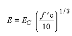
PDF files can be viewed with the Acrobat® Reader®

Chapter 2. Theoretical Manual

Bulk and Shear Moduli

Young's modulus of concrete varies with concrete strength, as shown in Table 1. These measurements are taken from an equation in CEB, as shown in Figure 74:

Figure 74. Equation. Default Young's modulus E.

Here, E is Young's modulus and E_C = 18.275 MPa (2,651 psi) (which is the value of Young's modulus when f ' c = 10 MPa (1,450 psi)). This value of E_C is for simulations that are modeled linear to the peak (no prepeak hardening). Poisson's ratio is typically taken as being between 0.1 and 0.2. A value of η = 0.15 is selected here and is assumed to remain constant with concrete strength. Based on this information, the default bulk and shear moduli (K and G) in Table 1 are derived from the classical relationships between stiffness constants, as shown in Figure 75:

Figure 75. Equation. Shear and bulk moduli, G and K.

The equations in Figure 74 and Figure 75 are implemented in the concrete model initialization routines to set the default moduli of concrete as a function of concrete compressive strength.

Alternatively, the ACI Committee 318 suggests the formula shown in Figure 76 for the elastic modulus:

Figure 76. Equation. ACI Young's modulus, E_c.

where w_c is the density of concrete in kilograms per meters cubed (kg/m³). For normal weight concrete with w_c = 2,286 kg/m³ (5,040 pounds per feet cubed (lb/ft³)), this formula reduces to the equation shown in Figure 77:

Figure 77. Equation. Reduced ACI Young's modulus, E_c.

This formula gives Young's moduli that are within ±9 percent of those given by Figure 74, as shown in Table 2.

Triaxial Compression Surface

The TXC yield surface equation is fit to four strength measurements. For roadside safety applications, the regimes of interest are primarily the tensile and low confining pressure regimes. Hence, the first and most common measurement fitted is unconfined compression, in which the pressure is one-third the strength. The second measurement is uniaxial tension, which is often called direct pull. The third measurement is triaxial tension (equal tension in three directions), which sets the apex of the TXC yield surface. The fourth measurement is TXC at a specified pressure. The pressure selected is 70 MPa (10,153 psi). The fit to this measurement anchors the yield surface at low to moderate pressure.

Strength measurements are given in Table 3. The uniaxial compression and tension measurements are taken from tables and information provided in CEB. The triaxial tension measurement is equal to the uniaxial tension measurement. This choice, along with appropriate selection of the three-invariant scale factors, will model the biaxial tension strength approximately equal to the uniaxial tension strength. This is the recommendation in CEB.

The TXC measurement (principal stress difference) is taken from a review of test data. For example:

• Measurements made for three similar concretes with f 'c = 45 MPa (6,527 psi) indicate an average triaxial strength of about 120 MPa (17,405 psi) (principal stress difference) at a pressure of 69 MPa (10,008 psi).⁽²⁵⁾

• Measurements reported by reference 28 for normal strength concrete with f '_C = 25 MPa (3,626 psi) indicate a principal stress difference of 69 MPa (10,008 psi) at a pressure of 37 MPa (5,366 psi).

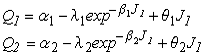
The TXC yield surface equation relates strength to pressure via four parameters as shown in Figure 78:

Figure 78. Equation. TXC Strength.

At each value of unconfined compressive strength, the four strength parameters (α, λ, β, θ) are simultaneously fit to the four strength values via an iterative procedure. Fitted values at five strengths are given in Table 4.

Obviously, a user may wish to analyze concrete at strengths other than the five listed. To accomplish this, quadratic equations as a function of unconfined compression strength are fit through each parameter, P, as shown in Figure 79:

Figure 79. Equation. Interpolation parameter P.

For the TXC yield surface, the parameter P represents either α, λ, β, or q. The fitted values of A_P, B_P, and C_P are given in Table 5. Fitted values of A_P, B_P, and C_P for all other concrete model input parameters (TOR and TXE yield surfaces, cap, damage, rate effects parameters) are given in subsequent sections.

MPa^-1 = 0.006895 psi^-1

Triaxial Extension and Torsion Surfaces

The Rubin scaling functions determine the strength of concrete for any state of stress relative to the TXC strength.⁽¹⁷⁾ The strength ratios are shown in Figure 80:

Figure 80. Equation. Most general form for Q₁, Q₂.

where Q₁ is the TOR/TXE strength ratio, and Q₂ is the TXE/TXE strength ratio. Each ratio may remain constant or vary with pressure. The default fits of these equations to data are given in Table 6 and Table 7, and are based on the following data and assumptions:

• The shape of the yield surface in the deviatoric plane is triangular when the pressure is tensile. This means that Q₁ = 0.5774 and Q₂ = 0.5. In this case, Q₁ and Q₂ are set internally, and the values of α_λ,λ_λ,β_λ, θ_λ, and α₂,λ₂,β₂, θ₂ are not used. These fits model biaxial tensile strengths that are within 1 percent of the uniaxial tensile strengths, as specified in CEB.
• The shape of the yield surface in the deviatoric plane transitions from a triangle at P = 0 to an irregular hexagon for P > 0. In this case, Q₂ is set to give a biaxial compression strength that is approximately 15 percent larger than the uniaxial compressive strength (f '_BC = 1.15f '_C ), as specified in CEB. This CEB specification agrees with the data of reference 16. This reference suggests a biaxial compressive strength that is approximately 16 percent higher than the unconfined compressive strength.
• The fits in tension and compression will smoothly intersect at values of Q₁ = 0.5774 and Q₂ = 0.5 in pure shear (P = 0).

MPa^-1 = 0.006895 psi^-1

MPa^-1 = 0.006895 psi^-1

Again, because users may want to analyze concrete at a strength other than the five listed, quadratic equations as a function of unconfined compression strength are fit through each set of parameter values for the TOR and TXE surfaces. The quadratic equation coefficients were previously given in Table 5.

Cap Location, Shape, and Hardening Parameters

The cap parameters are selected by fitting pressure-volumetric strain curves measured in hydrostatic compression and uniaxial strain tests. Default fits, given in Table 8, are based on the following data and assumptions:

• The initial cap location is the pressure invariant at which the hydrostatic pressure-volumetric strain curve becomes nonlinear. Nonlinearity initiates at lower pressures for lower strength concrete. Hence, the initial cap location decreases with decreasing concrete strength.
• The cap shape, combined with the initial cap location, sets the pressure at which the uniaxial-strain pressure-volumetric strain curve becomes nonlinear. A cap shape parameter of 5 is typical and is commonly used by the developer to fit concrete with f ' c = 45 MPa (6,527 psi).
• The maximum plastic volume change sets the range in volumetric strain over which the pressure-volumetric strain curve is nonlinear (from onset to lock-up). Typically, the maximum plastic volume change is approximately equal to the porosity of the air voids. A value of 0.05 indicates an air void porosity of 5 percent. It is not expected that the pores in roadside safety applications will compact fully. Therefore, this parameter is judgmentally set to provide a reasonably shaped pressure-volumetric strain curve in the low-to-moderate pressure regime applicable to roadside safety testing.
• The linear cap hardening parameter sets the shape of the pressure-volumetric strain curve, although it produces a sudden transition at the onset of nonlinearity. The quadratic cap hardening parameter smoothes this transition.

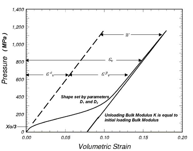
An example pressure-volumetric strain curve from an isotropic compression simulation is given in Figure 81. This figure demonstrates how each parameter affects the shape of the curve.

The cap initial location varies with compressive strength. The quadratic equation is used to obtain the cap location at a compressive strength other than the five tabulated. The quadratic equation coefficients are: A_P = 8.769178e-03 MPa^-1, B_P = -7.3302306e-02, and C_P = 84.85 MPa (12,306 psi).

psi = 145.05 MPa

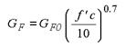
psi = 145.05 MPa

Figure 81. Graph. This isotropic compression simulation demonstrates how the cap parameters set the shape of the pressure-volumetric strain curve.

Damage Parameters

Concrete softens in the tensile and low confining pressure regimes. For modeling purposes, fracture energy is defined as the area under the softening portion of a stress-displacement curve from peak stress to complete softening. One equation in CEB relates the measured fracture energy in tension to the unconfined compression strength and the maximum aggregate size, as shown in Figure 82:

Figure 82. Equation. The default fracture energy G_F.

KPa-cm = kilopascals-centimeters

1 KPa-cm = 0.05710 Psi-inch

Here G_F0 is the fracture energy at f ¢c = 10 MPa (1,450 psi) as a function of the maximum aggregate size. CEB actually lists the value of G_F0 as 5.8 for 32-mm (1.26-inch) aggregate, but it has been replaced with 3.8 to make G _F consistent with CEB tabulated values. The fit of the quadratic equation to these G_F0 values as a function of aggregate size in mm is A_P = 0.000520833 cm/KPa, B_P = 0.75 cm, and C_P = 1.9334 KPa-cm.

Tensile fracture energies calculated from the equation in Figure 82 at five specific concrete strengths are given in Table 10.

1 KPa-cm = 0.05710 Psi-inch

The concrete material model requires specification of the fracture energies in uniaxial tensile stress, uniaxial compressive stress, and pure shear stress. Default values for the tensile fracture energy are given by the equation in Figure 82. Default values for the compressive fracture energy are set at 100 times the tensile fracture energy. Default values for the shear fracture energy are set equal to the tensile fracture energy.

Other input parameters required are the brittle and ductile damage thresholds and the maximum damage levels:

• Each damage threshold sets the elastic strain energy level at which softening initiates. The brittle damage threshold is set equal to the elastic strain energy level in unconfined tension at peak stress. The ductile damage threshold is set equal to the elastic strain energy level in unconfined compression at peak stress.
• The shape of the softening curves is set by the parameters B and D. A value of B = 100.0 is set in compression for gradual initial softening (flat top). A value of D = 0.1 is set in tension for brittle initial softening (pointed top).
• The maximum damage parameters set the maximum damage levels attained in unconfined compression and tension. The maximum damage levels are set equal to 0.99 for both brittle and ductile formulations.

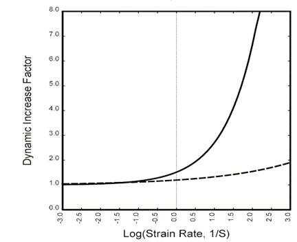
Strain Rate Parameters

Concrete exhibits an increase in strength with increasing strain rate (refer to Figure 13 and Figure 14). Data are typically reported in terms of the ratio of dynamic to static strength, called the dynamic increase factor (DIF). CEB provides specifications for the DIF, as discussed in appendix D. However, the CEB specifications are not a good fit to the tensile data previously shown in Figure 14. Therefore, the DIF used and shown in Figure 83 is based on the developer's experience on various defense contracts, particularly for concrete with strength around f 'c = 45 MPa (6,527 psi). These specifications provide a good fit to both the tension and compression data previously shown in Figure 13 and Figure 14.

DIF specifications are approximately met by running numerous calculations and selecting the viscoplastic rate effects parameters via a trial and error method. The viscoplastic parameters are applied to the plasticity, damage, and fracture energy formulations. These parameters are η_0t and n_t for fitting uniaxial tensile stress data, and η_0c and n_c for fitting uniaxial compression data. Quadratic equation coefficients are dependent on the unconfined compression strength, but are independent of the aggregate size.

The default parameters in tension are n_t = 0.48, with quadratic equation coefficients for η_0t of A_P = 8.0614774E-13, B_P = −9.77736719E-10, and C_P = 5.0752351E-05 for time in seconds and stress in pounds per square inch. The default parameters in compression are n_c = 0.78, with quadratic equation coefficients for η_0c of A_P = 1.2772337-11, B_P = −1.0613722E-07, and C_P = 3.203497-04. Rate effects parameters in pure shear stress are set equal to those in tension via Srate = 1.

The overstress limits in tension (overt) and compression (overc) limit rate effects at high strain rates ( > 100). The overstress quadratic equation coefficients for overt are A_P = 1.309663E-02 MPa^-1, B_P = −0.3927659, and C_P = 21.45 MPa. These provide tensile and compressive overstress limits of 21 MPa (3,046 psi) at an unconfined compression strength of 30 MPa (4,351 psi).

The literature contains conflicting information about whether fracture energy is strain rate dependent. One possibility is to model the fracture energy independent of strain rate (repow = 0). Another possibility is to increase the fracture energy with strain rate by multiplying the static fracture energy by the DIF (repow = 1). The developer's experience has been to increase the value of the fracture energy with strain rate; hence, repow = 1 is the default value. This value provides good correlations with test data for most of the problems analyzed and discussed in the companion concrete model evaluation report.⁽¹⁾ However, the Texas T4 bridge rail simulations correlate best with data if the fracture energy increases with the square root of the strain rate (repow = 0.5).

Units

Five systems of units are provided. These are:

• EQ. 0. GPa, mm, milliseconds, kg/mm³, kilonewtons (kN)
• EQ. 1. MPa, mm, milliseconds, grams per millimeter cubed (g/mm³), newtons (N)
• EQ. 2. MPa, mm, seconds, milligram per mm³ (mg/mm³), N
• EQ. 3. psi, inch, seconds, pound-seconds squared per inch to the fourth (lb-s²/inch⁴), lb
• EQ. 4. Pa, m, seconds, kg/m³, N

Previous | Table of Contents | Next