U.S. Department of Transportation
Federal Highway Administration
1200 New Jersey Avenue, SE
Washington, DC 20590
202-366-4000
Federal Highway Administration Research and Technology
Coordinating, Developing, and Delivering Highway Transportation Innovations
| REPORT |
| This report is an archived publication and may contain dated technical, contact, and link information |
|
| Publication Number: FHWA-HRT-15-074 Date: September 2016 |
Publication Number: FHWA-HRT-15-074 Date: September 2016 |
The main purpose of the field evaluation was to establish the precision and accuracy of the devices considered in this study. A diary of the field activities, including a detailed description of how data were collected, is included in appendix B of this report. Data collected in the field included TSDD data, embedded sensor data, environmental data, and high-speed videos. This chapter describes the process of collecting, reducing, and analyzing the raw data as well as the development of a database. It also covers different methodologies used to evaluate the precision and accuracy of both devices.
The MnROAD facility was selected as the primary site since it provided a multitude of test sections in one location. The facility consists of a 3.5-mi (5.6-km) mainline roadway (see figure 20) comprising 45 sections with live traffic as part of Interstate 94 near Albertville, MN. In addition, a 2.5-mi (4-km) closed-loop low-volume road (LVR) containing 28 sections was also available (see figure 21). The section lengths were typically about 500 ft (152.5 m) long.

Source: Benjamin Worel
Figure 20. Illustration. MnROAD mainline test cell map.

Source: Benjamin Worel
Figure 21. Illustration. MnROAD LVR test cell map.
Table 14 provides a summary of the pavement structure information for the MnROAD test sections. The sections varied in pavement type, with the mainline consisting of 13 AC sections, 15 PCC sections, 14 white-topping sections, and 3 Strategic Highway Research Program composite sections and the LVR consisting of 15 AC sections and 13 PCC sections.
| Section | Pavement Structure | Layer Thickness (inches) | Section Length (ft) | ||||
|---|---|---|---|---|---|---|---|
| Minimum | Maximum | Average | Minimum | Maximum | Average | ||
| Mainline | Asphalt | 3 | 6 | 4.9 | 462 | 500 | 496 |
| PCC | 5 | 9.5 | 6.6 | 210 | 512 | 374 | |
| Stabilized full-depth reclamation (FDR) | 6 | 8 | 6.7 | 454 | 500 | 485 | |
| Unbound concrete overlay | 7.5 (PCC) | 7.5 (PCC) | 7.5 (PCC) | 117 | 153 | 137 | |
| 5 (AC) | 5 (AC) | 5 (AC) | |||||
| White-topping | 4 (PCC) | 6 (PCC) | 5.6 (PCC) | 24 | 449 | 137 | |
| 5 (AC) | 8 (AC) | 6.9 (AC) | |||||
| LVR | Asphalt | 3 | 5.5 | 4.1 | 225 | 507 | 389 |
| PCC | 4 | 12 | 7 | 118 | 508 | 377 | |
1 inch = 25.4 mm
1 ft = 0.305 m
In addition to the test sections along the mainline and LVR of the MnROAD, an 18-mi (29-km) loop of Minnesota roadway network in Wright County, MN, (see figure 22) was also tested. The loop was located about 20 mi (32 km) from the MnROAD facility and separated into nine sections. MnDOT (through Wright County) provided the pavement structure and IRI data in support of the TSDD study (see table 15). As is the case for many realistic pavement evaluation, a part of section 9 was under construction that might have led to an unanticipated slow down or lane change in a short segment of that section. In addition to providing realistic test sections, the loop also contained tight turns and rolling hills that provided data to evaluate the effects of horizontal and vertical curves.
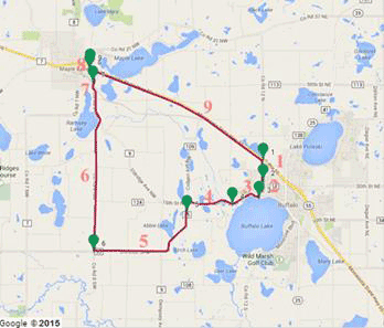
©2015 Google® (Modifications: See Acknowledgements).
Figure 22. Map. Testing loop in Wright County, MN.(41)
| Section | Length (mi) | Layer Thickness (inches) | Average IRI (inch/mi) | ||
|---|---|---|---|---|---|
| AC | Base | Subbase | |||
| 1 | 0.6 | 3.5 | 10 | - | 57 |
| 2 | 0.5 | 4.0 | 13 | - | 70 |
| 3 | 0.9 | 3.5 | 10 | - | 57 |
| 4 | 1.6 | 3.5 | 10 | - | 51 |
| 5 | 3.6 | 7.0 | 3 | 5 | 146 |
| 6 | 5.0 | 8.3 | 12 | - | 146 |
| 7 | 0.4 | 5.5 | - | - | 146 |
| 8 | 0.1 | 4.5 | 5 | 10 | 310 |
| 9 | 5.8 | N/A | N/A | N/A | 89 |
1 mi = 1.61 km
1 inch = 25.4 mm
1 inch/mi = 15.8 mm/km
N/A = Not available.
- Layer was not present.
The MnROAD sections were instrumented with different types of sensors, such as LVDTs, strain gauges, pressure cells, moisture gauges, thermocouples (TCs), and tipping buckets. Distress surveys, rutting measurements, laser profiler measurements, and FWD data were collected regularly on the sections. In addition to existing sensors, four geophones and one accelerometer were installed as embedded sensors to measure deflection velocity and displacement parameters at four MnROAD cells. Based on the criteria discussed in section 4.2 and in consultation with MnROAD staff, three flexible and one rigid pavement sections were selected. The pavement cross sections for the four cells are included in figure 23. The three flexible pavement sections covered three levels of stiffness (cell 34 soft, cell 19 intermediate, and cell 3 stiff as judged by FWD testing and pavement structure). Geophones were primarily used since they are the least expensive and can be easily ruggedized in a steel casing as well as due to their one-to- one correspondence to the deflection parameters measured by the TSD. In addition, one accelerometer was used at each site to verify the responses of the retrofitted geophones. The geophones had nominal resonant frequencies of 4.5 Hz and a measuring range of 160 mil (4 mm). The accelerometers were micro-electro-mechanical system direct current accelerometers with a nominal sensitivity of 28,350 mV/oz (1,000 mV/g). Aluminum holders were machined to provide them the protection needed to withstand the testing process. The geophones were calibrated using a shaker table and a high-precision reference accelerometer to establish their frequency responses after they were placed in the metallic holders.
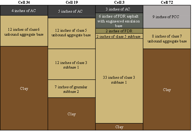
1 inch = 25.4 mm
Figure 23. Illustration. Pavement structure cross section of accuracy cells.
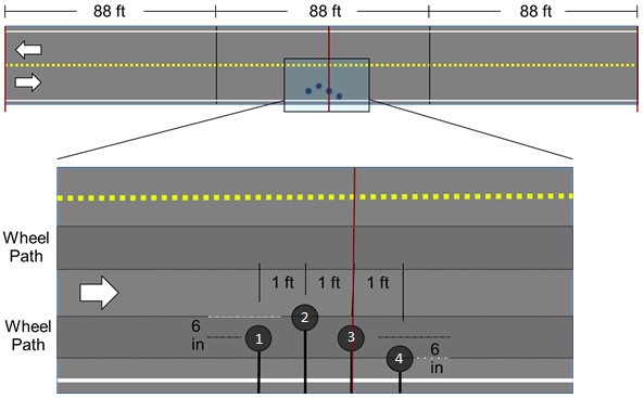
Geophones and accelerometers were embedded in the right wheel path of each selected MnROAD cell, as shown in figure 24. Two of the geophones (marked as 1 and 3) were installed along the center of the wheelpath, while the other two (marked as 2 and 4) had 6 inches (152.4 mm) offset to either side of the wheelpath center. The purpose for this offset was to increase the probability of having the test vehicle sensor pass directly on top of one of the sensors while data from the test vehicle and embedded sensors were being collected. The accelerometer was packaged with geophone 3.
1 ft = 0.305 m
1 inch = 25.4 mm
Figure 24. Illustration. Typical test section of MnROAD cell.
As illustrated in figure 25 through figure 28, 5 sensors were installed at each cell (3, 19, 34, and 72) for a total of 20 sensors. The activities associated with installing the five sensors at each cell included the following:
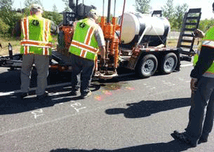
Figure 25. Photo. Pavement coring for sensor installation.
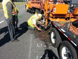
Figure 26. Photo. Smoothing of holes for sensor installation.
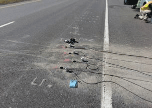
Figure 27. Photo. Grooving of pavement for sensor installation.
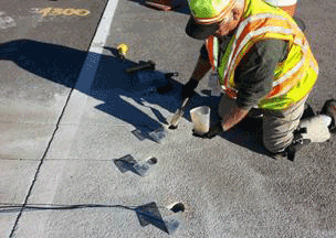
Figure 28. Photo. Partial grouting of the sensors.
As shown in figure 29 and figure 30, the performance of each sensor was then verified using an FWD. For that purpose, one of the FWD sensors was placed directly on top of one of the embedded sensors. The deflections reported by the FWD were then compared with the corresponding deflections reported by the embedded geophones and accelerometers.
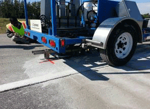
Figure 29. Photo. Alignment of project sensor with FWD sensor.
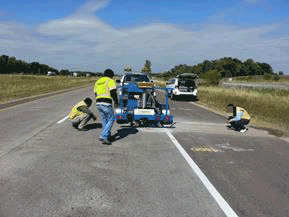
Figure 30. Photo. Sensor verification with FWD.
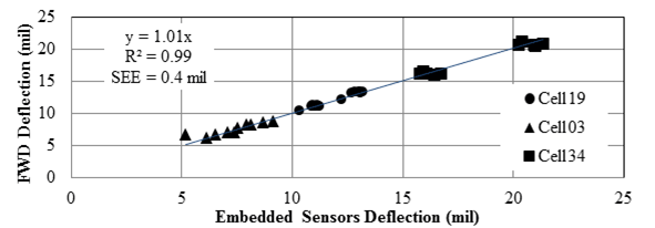
The results from the sensors installed at the three flexible pavement MnROAD cells are presented in figure 31. The deflections from the FWD sensors and the embedded sensors were quite similar. The typical accuracy of the geophones similar to those used in the FWD and installed at MnROAD was reported by the manufacturer as 2 percent of the measured deflection (no less than ±0.2 mil (0.0051 mm)). Based on the reported statistics in the figure, on average, the deflections of the FWD and installed sensors were within about 0.4 mil (0.010 mm) of one another, which confirms the adequacy of the installed system given the uncertainty associated with measurements with short impulse tests (i.e., FWD).
1 mil = 0.0254 mm
SEE = Standard error of estimate.
Figure 31. Graph. Evaluation of performance of embedded sensors with FWD.
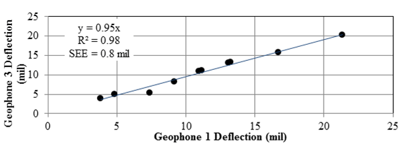
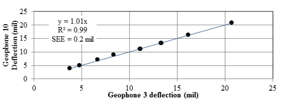
Figure 32 shows a comparison of the FWD deflections on top of geophones 1 and 3 from the same exercise. The average difference between the deflections from the two geophones was about 5 percent with an SEE of 0.8 mil (0.02 mm). Figure 33 compares the deflections measured with FWD geophones 3 and 10, located at offsets of 12 and -12 inches, respectively, at the same time and indicates a difference of 1 percent with an SEE of about 0.2 mil (0.005 mm). A review of the data indicated that the reason for the higher uncertainty in the embedded sensors data was related to the inconsistency in the data of one of the embedded sensors at cell 34.
1 mil = 0.0254 mm
Figure 32. Graph. Comparison of deflections for embedded geophones 1 and 3 under FWD loading.
1 mil = 0.0254 mm
Figure 33. Graph. Comparison of deflections for FWD geophones 3 and 10.
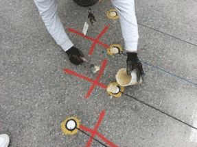
After verification of the performance of the embedded sensors, the sensors were then fully grouted (see figure 34). The feasibility of aligning the tires of the moving deflection devices with the sensors was also verified using the MnROAD instrumented truck (see figure 35).
 Â
Â
Figure 34. Photo. Final grouting of sensors.
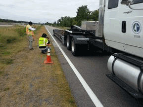
Figure 35. Photo. Verifying the embedded sensor alignment.
To properly trigger the embedded sensors, infrared light-emitting diode (LED) positioning sensors were installed in each of the accuracy testing cells. Figure 36 shows a typical layout of a test section with the positioning sensor arrangement. The positioning sensors consisted of a retro-reflective long-range sensor and a reflector. The sensor was encased in a protective box that was mounted on a metallic base that provided stability and could be maneuvered as needed. The reflector was also mounted on a similar base that offered the same benefits. These sensors had a sensing distance of up to 23 ft (7.02 m) and worked with 12 Vdc with an output pulse of the same amplitude.

1 ft = 0.305 m
Figure 36. Illustration. Test section layout with positioning sensors placement.
Markings for the trigger sensor positions were placed on the rest of the cells where accuracy testing was to be performed. The data acquisition (DAQ) system program was also modified to capture them in the data files. One positioning sensor was placed directly across from sensor unit 3 (geophone 3), a second positioning sensor was placed 132 ft (40.26 m) before sensor unit 3, and a third positioning sensor was placed 132 ft (40.26 m) after sensor unit 3. The reason behind the trigger spacing was the need to collect at least 3 s of information on each pass. The fastest vehicle speed proposed for testing (i.e., 60 mi/h (96.6 km/h)) resulted in a total length of 264 ft (80.52 m) for the test section. With this arrangement, the trigger sensor was placed 132 ft (40.26 m) before sensor unit 3 and was used to initiate the DAQ. The purpose for the trigger placed across sensor unit 3 was to use it as a reference to compare the shape of the deflection captured with the embedded sensors and the pulse width created by the tire as it crossed the trigger. Two high-speed video cameras were also used to record each pass of the TSDDs to determine the lateral wheel location relative to the installed sensors (see figure 37 and figure 38). The wheel wander for the passes that were used in this study were typically less than 2 inches (50.8 mm).
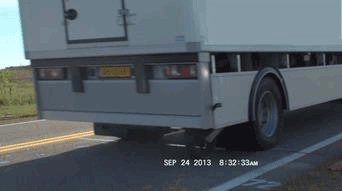
Figure 37. Photo. Sample video snapshot showing wheel location from TSD pass.
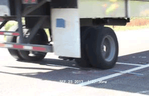
Figure 38. Photo. Sample video snapshot showing wheel location from RWD pass.
The DAQ system consisted of a National InstrumentsTM USB-6211 and a laptop. LabVIEW® software package also provided by National InstrumentsTM was used to develop the software needed to acquire, save, and analyze the data collected during the testing phase. During data collection, the only setting that needed to be modified was the speed of the vehicle before each test. This variable determined the amount of time needed to collect data with the DAQ system. MnROAD personnel provided the research team with an Arbiter Systems® GPS clock to ensure the collected data were correctly time stamped. While the TSDDs did not have this timing system, their computer clocks were sufficient to ensure their data as well as the data from the MnROAD sensors and installed sensors were correctly matched. To ensure the collected information was correctly assigned, the cell number, TSDD, vehicle speed, surface temperature, and repetition number were all used to name the files when data were saved. The project team encountered a problem while reducing data collected with the accelerometers for 15 out of 64 passes. The problem was tracked down to interference due to the absence of a ground connection, and the associated accelerometer data for the 15 passes in question were dropped from further consideration in the project.
Data collected were first subjected to a preliminary quality control. Quality control included classification and discarding of defective or unnecessary data for the purpose of this project. Since not all existing MnROAD embedded sensors were operational, their data were first visually inspected to identify the sensors that were operational at each cell.
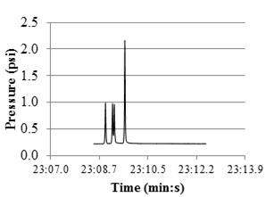
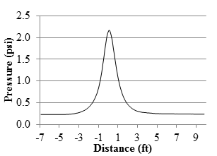
Typical examples of strain gauge and pressure cell data from one location are shown in figure 39 and figure 40. For each TSDD pass, the vehicle speed was calculated using the time between peaks generated by the front and the trailing rear axles and the exact distance between the axles. The vehicle speed obtained in that manner was then compared to the vehicle speed reported by the TSDD. The results were very comparable. Vehicle speed was then used to convert time into distance. Assuming that the peak value from the rear axle was obtained when the axle was directly on top of a sensor, data from -7 to 10 ft (-2.14 to 3.05 m) from the instant they occurred were extracted, as shown in figure 41 and figure 42. These extracted data were further summarized to discrete measurements at 1-ft (0.305-m) intervals to be uploaded into the project database. Given the viscoelastic nature of flexible pavements, a time lag between the time that the tire crosses over the sensor and when the maximum response is measured is anticipated. This time lag was ignored in the presentation of the strains and stresses in figure 39 through figure 42. However, the results were adjusted when the experimental results were compared with the numerical ones in chapter 7 of this report.
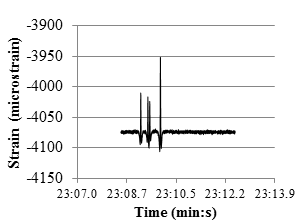
Figure 39. Graph. MnROAD strain gauge data.
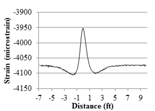
Figure 40. Graph. MnROAD strain gauge reduced data.
1 psi = 6.89 kPa
Figure 41. Graph. MnROAD soil compression gauge data.
1 psi = 6.89 kPa
1 ft = 0.305 m
Figure 42. Graph. MnROAD soil compression gauge reduced data.
Figure 43 shows a typical voltage time history obtained from an embedded geophone, with the peak voltage outputs created by the front and trailing rear axles marked. As with the other sensors, the time difference between the two peaks was divided by the front-axle-to-rear-axle distance of each TSDD to obtain accurate instantaneous vehicle speed, assuming that the time lags between the maximum displacement parameters and the time the tire passed over a sensor was constant for the front axle and the trailing rear axle.
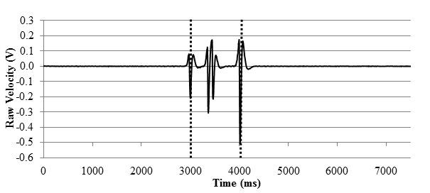
Figure 43. Graph. Embedded sensor full time history with the peaks created by rear and front axles.
The next step of the data analysis was to extract the appropriate range of information from all five newly embedded displacement sensors before, during, and after the rear axle of the TSDD drove over them over an approximate range of -7 to 10 ft (-2.14 to 3.05 m) from sensor unit 3. Figure 44 shows the voltage time histories from the geophone and accelerometer in sensor unit 3 from a typical TSDD pass.
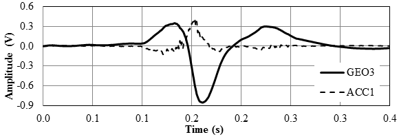
Figure 44. Graph. Geophone and accelerometer time histories.
Since the calibration values of the accelerometers were linear and constant, the accelerometer voltage time history was multiplied by the calibration value to convert it to acceleration. These data were first transformed into the frequency domain using an FFT algorithm integrated once in the frequency-domain to obtain the velocity spectrum and twice to obtain the deflection spectrum. The velocity or deflection spectrum was then subjected to an inverse FFT to obtain velocity or deflection time histories. The velocity results were compared to the TSD measured values, while the deflection results were compared with the RWD measurements.
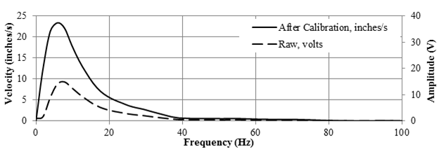
The process of analyzing the geophone data involved the use of the nonlinear calibration curve in the frequency domain obtained from the geophone calibration. Figure 45 shows a typical geophone calibration curve. Since the analysis process had to be done in the frequency domain, the first step was to use an FFT algorithm to convert the selected geophone time history from the time domain to the frequency domain. Figure 46 shows the voltage frequency spectrum of the time history of geophone 3 from figure 44, and it also shows the actual velocity spectrum obtained after dividing it by the calibration curve. The shift in the amplitude, especially at low frequencies, demonstrates the importance of implementing a rigorous calibration process to consider the nonlinear behavior of the geophone properly.

1 V/mil/s = 394 V/mm/s
Figure 45. Graph. Typical geophone calibration curve.
1 inch/s = 25.4 mm/s
Figure 46. Graph. Geophone velocity before and after calibration.
The actual velocity spectrum was then subjected to an inverse FFT algorithm to obtain the actual velocity time history that could be compared with those measured by the TSD. Figure 47 compares the raw geophone voltage time-history with the actual velocity time history, once again to demonstrate the importance of the proper analysis of geophone data. At this time, the time axis was also converted to distance as discussed previously.

1 inch/s = 25.4 mm/s
Figure 47. Graph. Geophone velocity before and after calibration in the time domain.
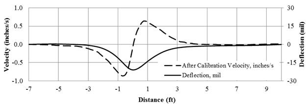
To obtain the deflection time history, the actual velocity spectrum illustrated in figure 46 was integrated in the frequency domain and then subjected to an inverse FFT algorithm. Figure 48 shows the analysis results from a typical geophone. Discrete results were extracted from the geophones and accelerometer data at spacings that matched the data reported by the TSDD. For the TSD, these distances included 60, 36, 24, 12, 8, and 4 inches (1,530, 914.4, 609.6, 304.8, 203.2, and 101.6 mm) from the applied load. For the RWD, two data points at -7.25 and 7.75 inches (-184.15 and 196.85 mm) from the applied load were extracted since the device measured vertical displacements with two sensors. The velocity, deflection, strain, and stresses from the MnROAD field sensors were also summarized by extracting the appropriate values at 12-inch (304.8-mm) increments. Based on figure 48 and other similar experiments, the measured deflections with the embedded geophones (and perhaps TSDD sensors) beyond ±2 ft (±0.61 m) were negligible and within the uncertainty band of the measurements.
1 inch/s = 25.4 mm/s
1 ft = 0.305 m
1 mil = 0.025 mm
Figure 48. Graph. Deflection velocity in spatial domain.
Figure 48 shows the typical velocities and deflections generated from the installed sensors by the TSDD rear axle after the analysis. The reported results from all sensors were confined to a distance of -7 to 10 ft (-2.14 to 3.05 m) from the instrumented TSDD rear axle right wheel while passing over the third geophone.
The peak velocities and deflections estimated from the accelerometer and geophone 3 of each cell (excluding the results from the earlier referenced 15 defective accelerometer records) are compared in figure 49 and figure 50, respectively. On average, the velocities from the two sensors differ by 3 percent, and the deflections differ by 7 percent. Even though the accelerometers collected data with less uncertainty than the geophones, the fact that the accelerometer raw data had to be integrated twice introduced more uncertainty in the analyses of deflections. The uncertainties in the reported values as judged by the SEE values are 30 mil/s (0.762 mm/s) and 1.5 mil (0.0381 mm), respectively. In the absence of definite means to attribute these uncertainties to the respective sources, they were fully attributed to the embedded sensors independent of their sources. Given the uncertainty associated with the data collection and analysis, the results were consistent.

1 inch/s = 25.4 mm/s
Figure 49. Graph. Geophone 3 and accelerometer velocity comparison.

1 mil = 0.025 mm
Figure 50. Graph. Geophone 3 and accelerometer deflection comparison.
Figure 51 and figure 52 compare the peak velocities and deflections from all the accuracy testing results from geophones 1 and 3. A few outliers are evident in the two graphs. The source of these outliers was traced to the inconsistency of the data for geophone 1 at cell 34. Based on these analyses, the TSDD results were compared to the geophone 3 results at each site. Including the outliers in the analysis, the velocities and deflections from the two sensors differed by about 1 percent on average. The uncertainties in the reported values as judged by the SEE values are 137 mil/s (3.5 mm/s) and 1.4 mil (0.036 mm), respectively. Again, these uncertainties were fully attributed to the embedded sensors and not other sources.

1 inch/s = 25.4 mm/s
Figure 51. Graph. Velocity comparison of geophones 1 and 3.

1 mil = 0.025 mm
Figure 52. Graph. Deflection comparison of geophones 1 and 3.
The three AC cells (3, 19, and 34) were used for accuracy analysis. The deflection measurements from PCC cell 72 were not considered because the slab did not show a localized deflection basin, and the magnitudes of the signals reported with the TSDDs and newly installed deflection sensors were too small to be accurate given their stated uncertainties. The accuracy was established by statistically comparing the results measured with the newly embedded sensors with those reported by the TSDDs. Since the TSDDs reported their averaged data at 32 ft (9.76 m) for TSD and 50 ft (15.25 m) for RWD, one-to-one comparisons of the measured and reported data were not possible. As such, the averaged data point closest to the embedded sensors was used for this purpose.
Figure 53 and figure 54 compare the TSD and the RWD discrete measured values with corresponding time histories from the embedded sensors, respectively. Since the TSD sensors measured the pavement surface velocity, the velocities measured with geophone 3 were compared with the TSD velocities in figure 53. On the other hand, the accuracy of the RWD was evaluated based on the deflections from geophone 3 since the RWD reports the surface displacements (see figure 54).

1 mil/s = 0.0254 mm/s
1 ft = 0.305 m
Figure 53. Graph. Comparison between embedded sensor deflection velocity results and TSD measurement.

1 mil = 0.0254 mm
1 ft = 0.305 m
Figure 54. Graph. Comparison between embedded sensor deflection results and RWD measurement.
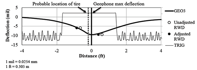
The viscoelastic nature of AC could result in a lag between the time that the tire crosses over the sensor and the time when the maximum response occurs. The deflection parameters shown in figure 53 and figure 54 consider such time lags. Figure 55 presents the process of obtaining this response lag. First, the most probable time that the center of the tire passed over the sensor was determined by estimating the distance where the trigger signal exhibited a high voltage (i.e., the length that the tire interfered with the LED laser reflection in figure 36). The resulting distance was then divided by two to estimate when the tire passed over the sensor (shown with a dotted vertical line in figure 55). The lag was then estimated by subtracting the estimated time when the TSDD sensor passed over the embedded sensor from the time when the maximum deflection measured with the geophone (solid vertical line) occurred. After calculating the lag for each pass, all data points were shifted accordingly. The estimated response lags are reported in table 16. Given the sampling rate of the newly installed geophone data and uncertainty in the process used, the uncertainty associated with the estimation of the phase lags was estimated to be 1–2 inches (25.4–50.8 mm). For the RWD passes, the response lags were estimated based on the measured deflections, while for the TSD, they corresponded to the surface particle velocities. The response lag varied with vehicle speed, temperature, and pavement structure. The time lags for cell 19 had to be determined differently since the body of the TSD interfered with the trigger signal. These time lags were approximated using an average wheel diameter of 3.2 ft (0.98 m) since the trigger signal for this cell covered both of the wheels (rear axle and the distant measuring instrument (DMI) wheel).
1 mil = 0.0254 mm
1 ft = 0.305 m
Figure 55. Graph. Time lag calculation example.
| Cell | Speed (mi/h) | Response Lag (inches) | |
|---|---|---|---|
| RWD | TSD | ||
| 34 | 30 | 7.3 | 3.8 |
| 45 | 6.9 | 3.4 | |
| 3 | 30 | 4.3 | 6.6 |
| 45 | 2.5 | 5.5 | |
| 60 | 1.6 | N/A | |
| 19 | 30 | 4.5 | 4.4 |
| 45 | 3.4 | 2.8 | |
| 60 | 4.0 | 2.8 | |
1 mi/h = 1.61 km/h
1 inch = 25.4 mm
N/A = Data were not available.
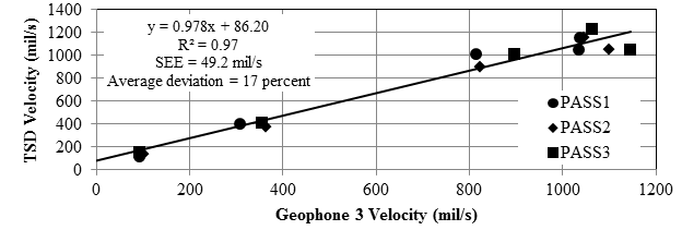
Figure 56 and figure 57 show typical comparisons between the parameters reported by the TSDDs and those measured by the newly installed embedded sensors. Given the inherent uncertainty in the acquisition and analyses of the embedded sensors' data, tests were repeated three times at every cell for every TSDD. The results from all three replicates were used to maximize the confidence in the data. The constant and the slope of the best fit line through the data were used to assess the closeness of the reported and measured results. The intercept measures the bias in the measurements and should ideally be equal to zero. For a fair comparison, the slope, which is an indication of the proportionality of the measurements, should be equal to unity. Average deviation between the measured and reference of a device under a given condition was also calculated by determining the absolute difference between the slope of the best fit line directed through the origin and the line of equality. An average deviation close to zero is desirable. The R2 value was examined as an approximate surrogate indicator of the scatter in the data since, strictly speaking, there are uncertainties in both the reference and measured values. Ideally, that value should be close to unity. In the case of RWD, R2 was not computed, as it contained only two measurements with repetition. The SEE was judged to be a better indicator of the uncertainty in the results. SEE can be used to estimate how different the deflection parameters from two different pavements should be so that they can be considered different with confidence. The smaller the SEE is, the more subtle changes in pavement structures can be estimated.
1 mil/s = 0.0254 mm/s
Figure 56. Graph. Comparison of geophone and TSD measurements.

1 mil = 0.0254 mm
Figure 57. Graph. Comparison of geophone and RWD measurements.
The individual difference between the deflection measured by the embedded sensor and the deflection reported by TSDD was estimated from the following:
![]()
Figure 58. Equation. Absolute difference between the deflection measured by the embedded sensor and the deflection reported by TSDD.
Where:
eij = Absolute difference between the deflection measured by the embedded sensor and the deflection reported by TSDD.
i = Sensor.
j = Pass.
dijsensor = Deflection parameter (either velocity or deflection) measured with the embedded geophone.
dijTSDD = Deflection parameter reported by the TSDD for its sensor i for pass j.
The average and standard deviation of differences from the three replicates for each sensor were then calculated and reported for each sensor (see table 17). For TSD, values from the sensor spacings of 36 and 60 inches (914.4 and 1,524 mm) were not evaluated since their deflection parameters were considered to be too small to be reliably measured by the embedded geophones.
| TSD | RWD | ||||
|---|---|---|---|---|---|
| Sensor Distance (inches) | Average Difference (Percent) | Standard Deviation of Difference (Percent) | Sensor Distance (inches) | Average Difference (Percent) | Standard Deviation of Difference (Percent) |
| 4 | 12 | 5 | -7.25 | 11 | 3 |
| 8 | 4 | 3 | 7.75 | 11 | 10 |
| 12 | 6 | 7 | |||
| 24 | 11 | 8 | |||
1 inch = 25.4 mm
Note: Since RWD only had two sensors, the results for the third and fourth sensors were left blank.
Table 18 summarizes the experiments carried out for establishing the accuracy of the TSDDs. The TSD was not able to test cell 3 at 60 mi/h (96.6 km/h) because of safety concerns over the breaking distance. Figures and tables similar to those presented over the remainder of this chapter and in chapter 6 were generated for every combination of device, cell, and nominal speed shown in table 18, but they were not included in the report, as they do not provide further insights. The data used to generate these figures and tables can be obtained directly from FHWA.
| Device | Cell | Nominal Speed (mi/h) |
|---|---|---|
| RWD | 3 | 30 |
| 45 | ||
| 60 | ||
| 19 | 30 | |
| 45 | ||
| 60 | ||
| 34 | 30 | |
| 45 | ||
| TSD | 3 | 30 |
| 45 | ||
| 19 | 30 | |
| 45 | ||
| 60 | ||
| 34 | 30 | |
| 45 |
1 mi/h = 1.61 km/h
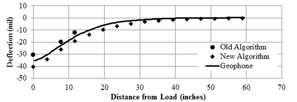
The deflection velocities were measured with the TSD. Most algorithms used for estimating the remaining life of pavement structures are based on deflection basins (usually measured with FWDs). To take advantage of the current procedures developed for the structural analysis of pavement structures, the TSD manufacturer suggested two algorithms. The typical outcomes of these two algorithms as well the deflection basins measured with geophone 3 are shown in figure 59. The first algorithm, labeled as “Old Algorithm,” is based on utilizing a beam model to estimate the deflection basins at three discrete points, including the deflection between the two wheels.(42,43) The second algorithm, labeled as “New Algorithm,” is based on the work by Pedersen et al. and utilizes the measured slope and fits this slope into a sum of two probability density functions to estimate the deflection basin up to 60 inches (1,524 mm) from the load.(44) The same process followed to estimate the accuracy of the TSD deflection velocity was also applied to the deflections estimated by the two algorithms, as discussed in chapter 6.
1 mil = 0.0254 mm
1 inch = 25.4 mm
Figure 59. Graph. Typical algorithm deflection comparison.
Precision analysis included almost all cells of the MnROAD facility and the 18-mi (29-km) Wright County loop to account for different pavement structures. To better evaluate the precision of the two devices, they were tested at different speeds and at different times of the day.
Table 19 describes the number of passes, speeds, and times for each device. Data collection was repeated up to five times at every cell for every TSDD and at two different speeds. Due to safety concerns, the LVR tests were carried out at nominally 30 and 45 mi/h (48 and 72 km/h). These combinations resulted in a total of 78 passes.
| Test Site | TSDD | Passes Per Speed | Speed (mi/h) | Time of Day |
|---|---|---|---|---|
| 18-mi loop | TSD | 3 | Traffic speed | Morning |
| RWD | 3 | Traffic speed | Morning | |
| Mainline | TSD | 5 | 45, 60 | Morning |
| 5 | 45, 60 | Afternoon | ||
| RWD | 3 | 45, 60 | Morning | |
| 3 | 45, 60 | Afternoon | ||
| LVR | TSD | 5 | 30, 45 | Morning |
| 5 | 30, 45 | Afternoon | ||
| RWD | 5 | 30, 45 | Morning | |
| 5 | 30, 45 | Afternoon |
1 mi = 1.61 km
1 mi/h = 1.61 km/h
Figures and tables similar to those presented over the remainder of this chapter and in chapter 6 were generated for every combination of test site, device, pass, speed, and time shown in table 19, but they are not included in the report, as they do not provide further insights. The data used to generate these figures and tables can be obtained directly from FHWA.
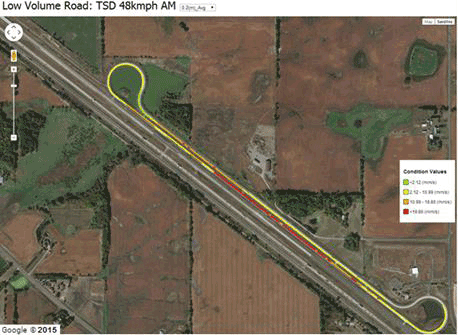
The precision analysis for this project started by developing color-coded Google® maps. An example of one of the maps is shown in figure 60. The average and COV of the deflection parameters for each sensor from replicate passes were calculated for each reported test point. These values were then color-coded using the convention in table 20. This color codification was also applied to the vehicle speed and pavement surface temperature measured by each TSDD since these parameters can influence the precision of the measurements.
©2015 Google® (Modifications: See Acknowledgements).
1 inch/s = 25.4 mm/s
1 mi/h = 1.61 km/h
Figure 60. Map. Color-coded statistic map.(45)
| Parameter | Color | |||
|---|---|---|---|---|
| Green | Yellow | Orange | Red | |
| Measurement | < Average - Standard Deviation | < Average but > Average - Standard Deviation | <Average + Standard Deviation but > Average | > Average + Standard Deviation |
| COV | < 5 percent | < 10 percent but > 5 percent | < 20 percent but > 10 percent | > 20 percent |
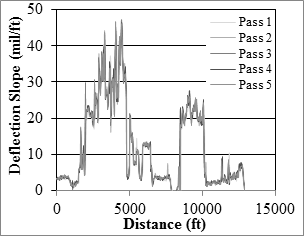
The first step to evaluate the precision was to properly align the starting point of each pass using the GPS coordinates provided by the TSDDs. The second analysis step consisted of comparing the deflection parameters from three or five replicate passes at similar speeds. For the RWD, the reported surface deflections were used for this purpose. The deflection slope, which is the ratio of the deflection velocity and vehicle speed (instead of deflection velocity that was used for the accuracy study), was used for the TSD. The TSD precision evaluation included the sensors from 4–36 inches (101.6–914.4 mm). Unlike the accuracy analysis, where small changes in the deflection parameter may yield high percent differences, the low precision (high variability) of the measurements can impact the analysis of the results negatively. Unlike deflection velocity, deflection slope can potentially reduce the impact of vehicle speed on the results. The appropriate deflection parameters (deflection for RWD and deflection slope for TSD) from different passes were first plotted and visually inspected to confirm the proper alignment of data (see figure 61). In some TSD passes, reported negative numbers were classified as measurement errors and were manually deleted to avoid misleading statistics.
1 mil/ft = 83.3 µm/m
1 ft = 0.305 m
Figure 61. Graph. Precision comparison of passes.
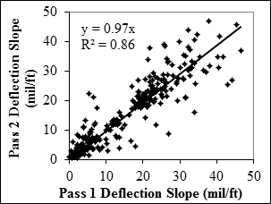
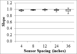
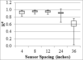
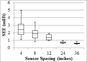
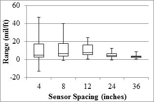
Statistical analyses were then carried out between each two individual pairs of data collected in different passes. As an example, figure 62 demonstrates a comparison of the data from the first and second passes of the TSD. Statistical parameters such as the R2 value, the slope of the best fit line, and the SEE were estimated for each pair, as shown in table 21. To summarize the extracted data in a manageable form, the minimum, maximum, and median values of each of these statistical parameters were extracted. These results were then presented as box plots. Typical box plots such as the ones presented in figure 63 through figure 66 demonstrate the ranges, 25 and 75 percentiles, and the medians for the slope, R2, SEE, and the range of measured values.
1 mil/ft = 83.3 µm/m
Figure 62. Graph. Precision linear comparison of passes.
1 inch = 25.4 mm
Figure 63. Graph. Typical slope box plot for precision analysis.
1 inch = 25.4 mm
Figure 64. Graph. Typical R2 box plot for precision analysis.
1 mil/ft = 83.3 µm/m
1 inch = 25.4 mm
Figure 65. Graph. Typical SEE box plot for precision analysis.
1 mil/ft = 83.3 µm/m
1 inch = 25.4 mm
Figure 66 . Graph. Typical range box plot for precision analysis.
| Pass Number | Pass 1 | Pass 2 | Pass 3 | Pass 4 | Pass 5 |
|---|---|---|---|---|---|
| Slope | |||||
| Pass 1 | 0.965 | 0.962 | 0.972 | 0.968 | |
| Pass 2 | 0.983 | 0.987 | 0.988 | ||
| Pass 3 | 0.992 | 1.003 | |||
| Pass 4 | 0.995 | ||||
| Pass 5 | |||||
| R2 | |||||
| Pass 1 | 0.864 | 0.878 | 0.911 | 0.887 | |
| Pass 2 | 0.957 | 0.965 | 0.959 | ||
| Pass 3 | 0.96 | 0.997 | |||
| Pass 4 | 0.967 | ||||
| Pass 5 | |||||
| SEE | |||||
| Pass 1 | 4.12 | 3.91 | 3.34 | 3.76 | |
| Pass 2 | 2.34 | 2.08 | 2.27 | ||
| Pass 3 | 2.27 | 0.65 | |||
| Pass 4 | 2.04 | ||||
| Pass 5 | |||||
Note: The blank cells correspond to the cells that do not require values as is the standard practice in elementary statistics.
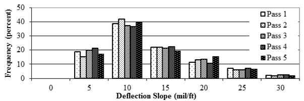
Histograms of the distributions of the reported parameters were also developed to visually evaluate the distributions of the data, as illustrated in figure 67.
1 mil/ft = 83.3 µm/m
Figure 67. Graph. Typical deflection for a particular sensor.
Such analyses were performed on the first five sensors of the TSD and the two sensors of the RWD. To further evaluate precision, the different passes were grouped together by time of the day (a.m. or p.m.), by speed (30, 45, or 60 mi/h (48.3, 72.45, or 96.6 km/h)), and by pavement structure (AC or PCC). The results from these analyses are presented in chapter 6. The RWD data files included the spatial standard deviations of the reported deflections over 50 ft (15.25 m), corresponding to the average values reported for each data point. The distributions of such spatial COVs for each measurement were also calculated and demonstrated. Such information was not available for the TSD.
Given the large quantity of data collected and reduced, a project database was needed to organize data analyses as well as to facilitate communication and accommodate the diverse needs of various team members working on the project. To that end, an online database was developed for ease of update and instant access to various data. The raw, reduced, and analyzed data from the accuracy and precision analyses were placed in the database. This database was also populated with other relevant data such as cell and sensor inventory, ambient conditions, pavement structure, and pavement condition (e.g., IRI measurements).
Figure 68 shows the homepage of the internal Web site containing the database. The structure of the database and the relevant schema and metadata is explained in a write-up within the database. The database is divided into the following sections:
This database was uploaded along with a folder containing all the linked data to a Web site developed for this project. The database and hence information contained therein may be obtained directly from FHWA.
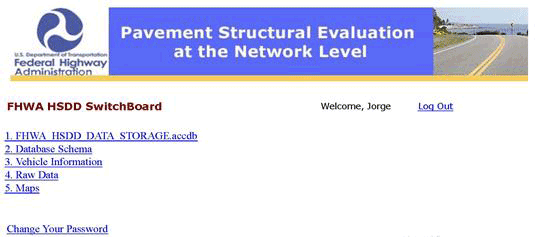
Figure 68. Screenshot. Database Web site homepage.
This chapter presents the field trial locations; the instrumentation used and retrofitted to evaluate the TSDDs; the methodologies used to collect, review, reduce, and analyze the data needed for quantifying the accuracy and precision of the TSDDs; and the effort required to store and manage the data so that potential users can take advantage of the wealth of data results generated in this study. These efforts were carried out to accomplish the following two objectives:
Considering the rationale provided in chapter 4 and the diverse data arranged and generated as discussed in this chapter, subsequent chapters are dedicated to elaborating on these two objectives.