U.S. Department of Transportation
Federal Highway Administration
1200 New Jersey Avenue, SE
Washington, DC 20590
202-366-4000


Skip to content
Facebook iconYouTube iconTwitter iconFlickr iconLinkedInInstagram

Federal Highway Administration Research and Technology
Coordinating, Developing, and Delivering Highway Transportation Innovations

Report
This report is an archived publication and may contain dated technical, contact, and link information
Publication Number: FHWA-HRT-08-057
Date: November 2008

Long-Term Pavement Performance Computed Parameter: Frost Penetration

APPENDIX A. E-FROST USER'S GUIDE

INTRODUCTION

This guide is designed to familiarize new users with the E-FROST user interface and analysis options. The guide includes screen captures to help the user navigate through the software screens.

E-FROST was designed to view time-series data from the in-situ measurements (ER, temperature, and moisture) used in frost penetration analysis, to generate and view frost penetration profiles, and to create frost penetration table documenting frost penetration depths for different dates for which in-situ measurements were taken.

E-FROST INSTALLATION AND REMOVAL

Complete the following steps to install E-FROST:

  1. Make sure that all other applications are closed and that the E-FROST installation CD-ROM has been inserted into the CD-ROM drive.
  2. From the Windows Start menu, select Run.
  3. In the Run dialog box, type "(CD drive):setup.exe," where (CD drive) is the letter assigned to your CD-ROM drive.
  4. Follow the simple instructions in the installation program. When installation is completed, E-FROST program will be available from the Start menu.

Complete the following steps to remove E-FROST:

  1. Click the Start button and choose the Settings option.
  2. Select Control Panel.
  3. From the Control Panel, double-click the Add/Remove Programs icon.
  4. Once within that dialog box, click the Install/Uninstall tab.
  5. Select E-FROST from the list of programs; then click the Add/Remove button.
  6. A final warning will ask if the user want to delete E-FROST from your computer. If this is the case, click Yes to remove all E-FROST files.

STARTING E-FROST

To start the program, click on E-FROST program name available from the Windows Start menu.

Main Form

When the E-FROST program is opened, a blank form with file menu and inactive tool buttons in the top left corner of the interface appears as shown figure 25.

This picture shows the opening screen in the computer program E-FROST. The screen consists of a mostly blank rectangular form with a file menu and inactive tool buttons in the top left corner of the interface.

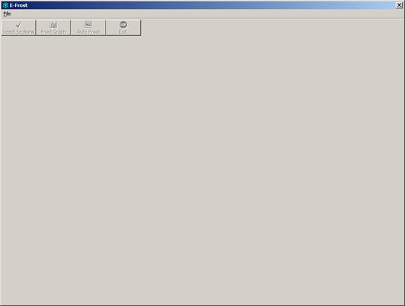
Figure 25. Screen capture. Opening screen in E-FROST.

There are four tool buttons in E-FROST that help navigate between screens and provide different program functions. These tool buttons are located on the left side of the screen and are shown in figure 26 . Each button's function is described below the figure.

This figure shows the four tool buttons that are available for use in E-FROST. From left to right, the buttons read Select Sections, Frost Graph, AutoFrost, and Exit. Each button has a graphic associated with it. The "Select Sections" button includes a picture of a check mark, the "Frost Graph" button includes a picture of a bar graph, the "AutoFrost" button includes a picture of an x-y plot, and the "Exit button" includes a picture of a stop sign.

Figure 26. Screen capture. Tool buttons.

Select Sections

The Select Sections tool button allows the user to choose a site for analysis from a list that is linked to the database.

Frost Graph

The Frost Graph tool button shows the frost graph after all missing temperature data and all temperature data between -1 °C and 0 °C have been reviewed. The Frost Graph button will be inactive until all review has taken place and the frost graph has been finalized.

Auto Frost

The Auto Frost tool button displays the frost graph with the original data set from the database before any review has taken place.

Exit

The Exit tool button safely closes the E-FROST program.

Load Database

To run E-FROST analyses, the analysis database needs to be loaded first. The analysis database contains preprocessed temperature, ER, and moisture data for the SMP sites. To load a database, click File > Open Database, as shown in figure 27 . A dialog box appears, prompting the user to open the database, as shown in figure 28 . After locating and selecting the database, click the Open button located in the bottom right portion of the dialog box.

This figure shows a screenshot of the "file" menu clicked. Under the file menu the first option, "Open Database," is selected and highlighted. Other options located under the file menu that are not selected include "Create Frost Penetration Table," which is an inactive option, and "Exit" which is an active option.

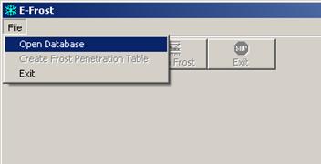
Figure 27. Screen capture. Open database.

This figure is a screenshot of the dialog box which appears after the user prompts the program to open the database. There is a drop down box at the top of the screen which the user can use to browse and locate the database. In this particular example, the database name is "Frost_Analysis_Database.mdb." In addition, there are icons on the left side of the screen for "My Recent Documents," "Desktop," "My Documents," "My Computer," and "My Network Places," which can assist the user in locating the database. The bottom right-hand corner of the screen contains "Open" and "Cancel" buttons. To the left of these buttons, the file name and file location are displayed in drop down boxes. Directly beneath the drop down boxes there is a check box that reads, "Open as read-only."

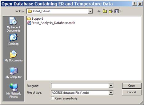
Figure 28. Screen capture. Locate the database containing SMP data.

Select Analysis Table

Once the analysis database is uploaded, the E-FROST analysis table selection window will appear as shown in figure 29 .

This figure is a screenshot of the E-FROST analysis table selection window. The upper left-hand side of the form reads, "Data Table." The upper middle of the form contains text box that includes the name of the selected file, which is "EFrostALL_QC" in this particular example. Directly below the text box containing the selected table, there is a list of all tables that are part of the selected database. To the right of the text box containing the selected table there are an "OK" button and a "Help" button.

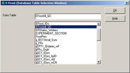
Figure 29. Screen capture. Select data table for analysis.

Select the table with the SMP site data, which is EFrostAll_QC and click OK to complete the database linking process. Once the database is connected to the program, the Select Sections and Exit user buttons will become active (figure 30 ).

This figure is a screenshot that consists of a mostly blank rectangular form with file menu and four tool buttons in the top left corner of the interface. The "Select Sections" and "Exit" tool buttons are shown active, while the "Frost Graph" and "AutoFrost" buttons are shown inactive.

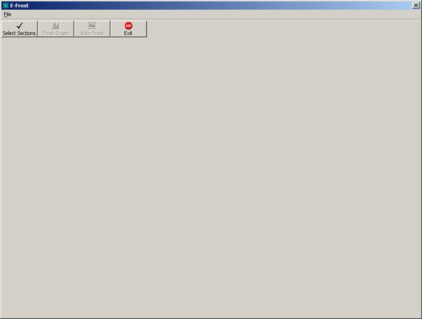
Figure 30. Screen capture. Frost linked to database with some tool buttons activated.

Select SMP Site

To select an SMP site for analysis, click the Select Sections tool button. A Section Selection window will appear containing a list of available SMP sections for analysis, as shown in figure 31 . Click an SMP section name and then click OK. In the following example SMP site 46-0804-1 was selected for analysis. The last digit in section ID represents LTPP construction number.

This figure is a screenshot of the "Select Sections" form. The left side of the form includes a list of available SMP sections. In this example, site "46-0804-1" is selected from the list and is highlighted. Above the list two rows of text read, "Available SMP Sections" and "Click to select." The upper portion of the form that is located to the right of the list has two rows of text that read, "Selected Sections" and "Double click to clear."  Below the text there is a box that lists all selected sections. In this example the only section in the list is "46-0804-1." Below the Selected Sections list there is a row of text that reads, "Note: Select only one Section at a time." Directly beneath the text there are two buttons. The button on the left reads "Clear Section" and the button on the right reads, "OK."

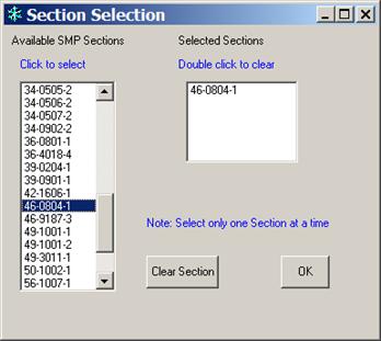
Figure 31. Screen capture. SMP Section window.

E-FROST ANALYSIS OPTIONS

Frost Penetration Analysis Form

A blank Frost Penetration Analysis form becomes visible once an SMP site is selected for analysis, as shown in figure 32 . If more than 2 years of data (730 days) are available for the site, a warning message will appear to prompt the user to select a shorter time period. The MinDate and MaxDate fields on the form indicate the range of the available data. Above the minimum and maximum dates are the text boxes where the user can enter date ranges for review. The user can move between different years of frost data by using the buttons to the right (to progress forward) or the left (to move backward) of the default user date range. The user can also manually enter the beginning and ending dates of interest by typing over the values in User Date boxes and clicking the Plot New button.

This figure is a screenshot of the form that the user will see after selecting a specific section in E-FROST. The top left corner of the form includes the file menu and four active tool buttons. The following fields are located below the tool buttons on the left hand side of the form: User Date, MinDate, MaxDate, No:, Depth, Date, FS, BS, No BS = 11, and (No BS) = 19. Each of these fields has a corresponding text box, with the exception of the User Date, which has two text boxes for a date range and the No:, which has a drop down menu. In addition, the User Date and No: fields have "<" and ">" buttons located to the left and right of their corresponding text boxes. The "<" and ">" buttons are used to jump between years and depth numbers. This portion of the form also has a button that reads, "Plot New." The following fields are located on the right-hand side of the form, below the tool buttons: ID, State, and Winter. The ID and State fields have one text box and the Winter field has two. Below all of the fields and buttons, and taking up the majority of the form, there is a blank x-y frost penetration graph, with the x-axis showing the date and the y-axis showing the depth in meters. The graph is titled, "Frost Penetration Analysis."

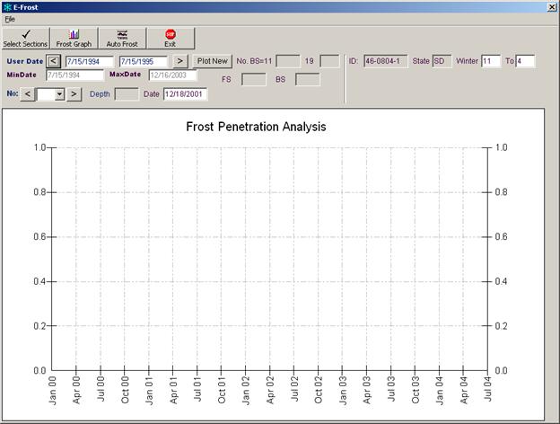
Figure 32. Screen capture. Blank Frost Penetration Analysis screen.

Review Auto Generated Frost Profile

Clicking on the Auto Frost tool button results in a generation of temperature-based frost penetration profile, as shown in figure 33 . In this example, the automated frost penetration profile was generated for SMP Site 46-0804 for the winter season of 1999–2000. The profile consists of a grid with the horizontal axis displaying different SMP dates on a daily scale and the vertical axis displaying different analysis depth based on ER probe depths. Each cell is color-coded to provide information about freeze state at a given date and at a given depth, as indicated in table 11 . In addition, black "X"s are used to indicate data points missing temperature data.

This figure is a screenshot of the form that the user will see after clicking the Auto Frost tool button for a specific site in E-FROST. In this figure, the automated frost penetration profile is generated for SMP Site 46-0804 with the user-defined date range from December 10, 1999, to March 16, 2000. The profile consists of a grid of color-coded cells, with the horizontal axis displaying different SMP dates on a daily scale and the vertical axis displaying different analysis depths based on ER probe depths in meters. Each cell is color-coded to provide information about freeze state at a given date and depth. The profile at this site consists of the three different freeze states: "Freeze," "No Freeze," and "To be Reviewed," which is where the temperature is between 0 degrees Celsius and -1 degrees Celsius. There are five separate areas of solid blue "Freeze" cells which begin in mid December and end in mid February, extending to a maximum depth of approximately 1 m. The "To be Reviewed" cells, denoted by light blue triangles, surround the solid blue freeze cells, making one continuous profile from mid December through early March and extending to a depth of approximately 1.2 m (3.9 ft). From late February to early March, the frost profile consists of "To be Reviewed" cells only, sandwiched between "No Freeze Cells," indicating the potential for a long spring thaw.

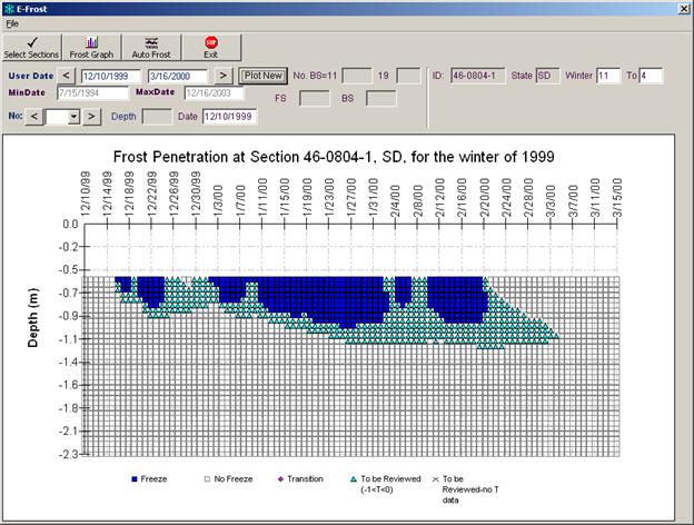
Figure 33. Chart. Automatically generated frost penetration profile at SMP site 46-0804 for the winter of 1999.

Table 11. Freeze state and frost depth chart color coding.
Color code Shape Assigned freeze state Subsurface temperature Analyst's action
Blue Rectangle Freeze T < -1 °C Assigned automatically; however, the analyst has an option to change the state to transitional (pink) or no-freeze (white) upon data review
White Rectangle No freeze T > 0 °C Assigned automatically; however, the analyst has an option to change the state to transitional (pink) or freeze (blue) upon data review
Light blue Triangle Review T < 0 °C and T > -1 °C Assigned automatically; however, the action is required from analyst to manually review the data and change the state to freeze, no-freeze, or transitional
Pink Diamond Transitional Near FR This color is assigned upon analyst review of all supporting data when it is not clear whether or not soil is frozen (partially frozen case)

The AutoFrost algorithm automatically assigns the state of subsurface freeze condition at each electrode location using the following rules:

Review Time Series Data

The light blue triangles on the AutoFrost profile graph indicate that the analyst must review the data and change the freeze state in the analysis table as appropriate. To aid in this analysis, E-FROST creates a time-series plot of ER, temperature, and moisture content changes. The plot is brought up to the screen once the analyst clicks on the light blue triangle cell. Similar plots can be brought up for review by clicking on any other cell on the frost penetration profile chart.

To review temperature, ER, and moisture time-series trends for a selected measurement depth, (1) identify measurement depth on left vertical axis in the frost penetration profile plot, then (2) click on any cell in the automated frost penetration graph for a selected depth value depth to bring up the time series graph (see the example shown in figure 34 ). Use the "<" and ">" buttons next to the No. label on the form to review the time series at different depths, or select the desired depth from the dropdown menu.

This figure contains an X-Y plot of Voltage, Resistance, Resistivity, TDR-MC, and Temperature data. The x-axis shows the date, while the left y-axis shows the normalized ER or MC value and the right y-axis shows the subsurface temperature in degrees Celsius. The x-axis covers the dates from December 5, 1999, through March 14, 2000. The temperature data are displayed using a solid purple line. The temperature data drop below 0 degrees Celsius in mid December and reach approximately -6 degrees Celsius near December 22. Around the end of December the temperature comes back up to 0 degrees Celsius and remains above 0 degrees Celsius until about January 1, which is when it dips back down below 0 degrees Celsius, reaching approximately -6 degrees Celsius. The temperature stays below 0 degrees Celsius, varying from 0 to -6 degrees Celsius until the end of February, which is when it becomes and stays greater than 0 degrees Celsius for the remainder of the profile. The TDR-MC values drop to near 0 around December 23, then rise as temperature increases briefly at the end of December, then decrease again from early to mid January. The TDR-MC values stay near 0 from January 12 to February 25. The TDR-MC values have a sharp increase at the end of February, as temperature values rise above 0 degrees Celsius. The ER data (which include navy blue upside-down triangles for the Voltage data and royal blue empty triangles for the Resistance data) are represented by individual points. The normalized ER data follow a trend almost opposite to temperature data, showing low values when the temperature is above 0 degrees Celsius and high values when the temperature is below 0 degrees Celsius, with exception of the period from mid to late December. The ER data do not follow the expected trend from mid to late December and stay near 0 when the temperature is below 0 degrees Celsius.

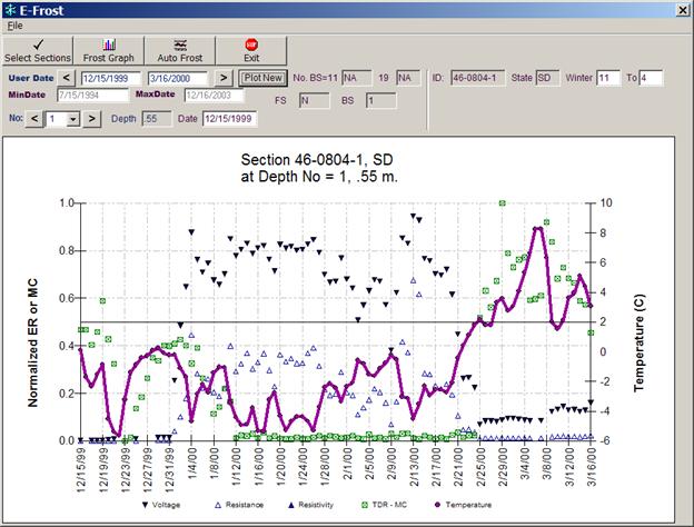
Figure 34. Chart. Time series plot for SMP site 46-0804 for the winter of 1999 at analysis depth = 0.55 m (1.8 ft).

Review Revised Frost Penetration Profile

Upon completion of the trend analysis and assignment of freezing conditions, an updated frost penetration plot can be reviewed by clicking on the Frost Graph tool button, as shown in figure 35 .

This figure shows a completed frost graph after review, with the x-axis showing the date and the y-axis showing the depth in meters. The user-defined date range is from December 10, 1999, to March 16, 2000. The profile consists of the three different freeze states: "Freeze," "No Freeze," and "Transition."  There are two separate areas that are identified as "Freeze" in the penetration profile. The first is from mid December to late December and extends to a depth of approximately 0.9 m (2.95 ft), and the second begins in early January and ends in early March extending to a depth of approximately 1.1 m (3.6 ft). The later part of the second freeze area includes a long thaw from about February 21 through the first week of March. During this thaw period, the frost profile shows deep frozen layers, while a no-freeze condition is shown close to the surface. A transitional period, indicated by pink cells, is shown between late December and early January, reaching a depth of approximately 0.9 m (2.95 ft). There are additional transitional cells located at the bottom of the frozen section from late January through late February at a depth of approximately 1.2 m (3.9 ft). These cells are located along the boundary differentiating between "Freeze" and "No Freeze" states.

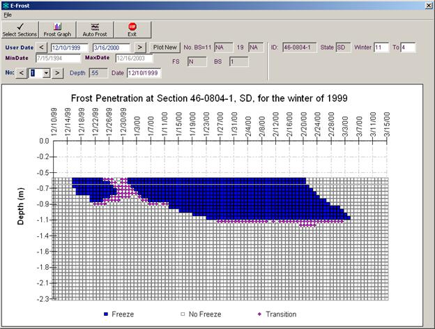
Figure 35. Chart. Final frost penetration profile for SMP site 46-0804 for the winter of 1999.

View Previously Processed Data

After the analysis of all sites is complete and all frost penetration profiles are finalized, the user can select any previously analyzed SMP site and view the frost penetration profiles at that site. To view previously processed data, click the Select Sections tool button and select an SMP site. Next, click the Frost Graph tool button to see the final frost penetration profile of the selected site. From the Frost Graph screen, the user can click on any cell to view the time series graph at selected depth. To view automatically generated frost penetration profile, click the Auto Frost tool button. To exit the program, click Exit on the tool bar.

GENERATE FROST PENETRATION TABLE

To generate the frost penetration table FrostPen, click File > Create Frost Penetration Table, as shown in figure 36.

This figure shows a screenshot of the "file" menu clicked. Under the File menu the second option "Create Frost Penetration Table" is selected and therefore highlighted. Other options under the File menu include "Open Database" and "Exit."

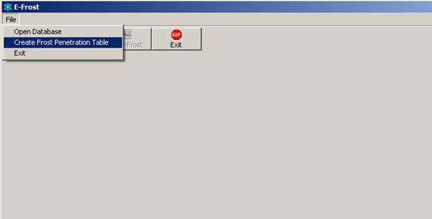
Figure 36. Screen capture. Create Frost Penetration Table option.

<< PreviousContentsNext >>


Federal Highway Administration | 1200 New Jersey Avenue, SE | Washington, DC 20590 | 202-366-4000
Turner-Fairbank Highway Research Center | 6300 Georgetown Pike | McLean, VA | 22101