U.S. Department of Transportation
Federal Highway Administration
1200 New Jersey Avenue, SE
Washington, DC 20590
202-366-4000
Federal Highway Administration Research and Technology
Coordinating, Developing, and Delivering Highway Transportation Innovations
 |
| This report is an archived publication and may contain dated technical, contact, and link information |
|
Publication Number: FHWA-HRT-04-046 Date: October 2004 |
Previous | Table of Contents | Next
There are several quality measures that can be used in an acceptance plan. In early QA specifications in the late 1960s and 1970s, the mean (or average), or the average deviation from a target value, was often used as the quality measure. However, the use of the average alone provides no measure of variability, and it is now recognized that variability is often an important predictor of performance. The problems associated with basing acceptance on only the mean are well documented. Therefore, there was no need to consider this approach in the analyses that were performed.
Several quality measures, including percent defective (PD) and PWL, have been preferred in recent years because they simultaneously measure both the average level and the variability in a statistically efficient way. Other measures that have been used by some agencies include AAD and the moving average. An additional measure that may be considered by some agencies is the CI.
PD and PWL are, in reality, the same quality measure since they are directly related by the simple relationship PWL = 100 - PD. Therefore, analyses reported using PWL also apply equally to PD, and vice versa.
The quality measures that were evaluated during the project include:
Since each of the above measures provides an estimate for a true population value, it is important to know that the estimator provides an unbiased estimate for the population parameter. It is known that this is true for the procedure for estimating PWL. Computer simulation was used to evaluate whether there was bias in any of the quality measures. A lack of bias means that the estimator is accurate. Another important factor to be considered is the variability associated with the quality measure (i.e., how much do individual estimated values vary about the long-term average value for the quality measure?) This, too, was investigated by computer simulation studies. Low variability for the estimated values is a sign that the estimator is precise.
Computer simulation studies were performed to evaluate the accuracy and precision of the estimated quality measures for various sample sizes. The results of these studies are presented for each measure in the following sections.
The PWL for a lot can be estimated by using the quality index, Q. The Q-statistic is used with a PWL table to determine the estimated PWL for the lot. A PWL table is shown in table 7.
Conceptually, the Q-statistic, or quality index, performs the same function
as the Z-statistic, except that the reference point is the mean of an
individual sample, ![]() ,
instead of the population mean,
,
instead of the population mean, ![]() , and the points of interest with regard to areas under the curve are the specification limits.
, and the points of interest with regard to areas under the curve are the specification limits.
 (1)
(1)
and
![]() (2)
(2)
where: ![]() =
quality index for the lower specification limit
=
quality index for the lower specification limit
![]() = quality index for the upper specification limit
= quality index for the upper specification limit
LSL = lower specification limit
USL = upper specification limit
![]() = sample mean for the lot
= sample mean for the lot
s = sample standard deviation for the lot
![]() is used when there is a one-sided lower specification limit, while
is used when there is a one-sided lower specification limit, while ![]() is used when there is a one-sided upper specification limit. For two-sided specification
limits, the PWL value is estimated as:
is used when there is a one-sided upper specification limit. For two-sided specification
limits, the PWL value is estimated as:
![]() (3)
(3)
where: PWLU = percent below the upper specification
limit (based on ![]() )
)
PWLL = percent above the lower specification
limit (based on ![]() )
)
PWLT = percent within the upper and lower specification limits
Computer simulation was used to generate samples of various sizes from known populations. These sample results were then used to estimate the PWL for the population. The mean and standard deviation for the estimated PWL values were then calculated. The difference between the mean estimated PWL was subtracted from the known population PWL to provide a measure of accuracy for the PWL estimates. The standard deviation of the estimated PWL values was used as a measure of precision (i.e., the amount of variability) for the PWL estimates.
Table 7. Quality index values for estimating PWL.
| PWL | n = 3 | n = 4 | n = 5 | n = 6 | n = 7 | n = 8 | n = 9 | n = 10 to 11 |
|---|---|---|---|---|---|---|---|---|
| 100 | 1.16 | 1.50 | 1.79 | 2.03 | 2.23 | 2.39 | 2.53 | 2.65 |
| 99 | - | 1.47 | 1.67 | 1.80 | 1.89 | 1.95 | 2.00 | 2.04 |
| 98 | 1.15 | 1.44 | 1.60 | 1.70 | 1.76 | 1.81 | 1.84 | 1.86 |
| 97 | - | 1.41 | 1.54 | 1.62 | 1.67 | 1.70 | 1.72 | 1.74 |
| 96 | 1.14 | 1.38 | 1.49 | 1.55 | 1.59 | 1.61 | 1.63 | 1.65 |
| 95 | - | 1.35 | 1.44 | 1.49 | 1.52 | 1.54 | 1.55 | 1.56 |
| 94 | 1.13 | 1.32 | 1.39 | 1.43 | 1.46 | 1.47 | 1.48 | 1.49 |
| 93 | - | 1.29 | 1.35 | 1.38 | 1.40 | 1.41 | 1.42 | 1.43 |
| 92 | 1.12 | 1.26 | 1.31 | 1.33 | 1.35 | 1.36 | 1.36 | 1.37 |
| 91 | 1.11 | 1.23 | 1.27 | 1.29 | 1.30 | 1.30 | 1.31 | 1.31 |
| 90 | 1.10 | 1.20 | 1.23 | 1.24 | 1.25 | 1.25 | 1.26 | 1.26 |
| 89 | 1.09 | 1.17 | 1.19 | 1.20 | 1.20 | 1.21 | 1.21 | 1.21 |
| 88 | 1.07 | 1.14 | 1.15 | 1.16 | 1.16 | 1.16 | 1.16 | 1.17 |
| 87 | 1.06 | 1.11 | 1.12 | 1.12 | 1.12 | 1.12 | 1.12 | 1.12 |
| 86 | 1.04 | 1.08 | 1.08 | 1.08 | 1.08 | 1.08 | 1.08 | 1.08 |
| 85 | 1.03 | 1.05 | 1.05 | 1.04 | 1.04 | 1.04 | 1.04 | 1.04 |
| 84 | 1.01 | 1.02 | 1.01 | 1.01 | 1.00 | 1.00 | 1.00 | 1.00 |
| 83 | 1.00 | 0.99 | 0.98 | 0.97 | 0.97 | 0.96 | 0.96 | 0.96 |
| 82 | 0.97 | 0.96 | 0.95 | 0.94 | 0.93 | 0.93 | 0.93 | 0.92 |
| 81 | 0.96 | 0.93 | 0.91 | 0.90 | 0.90 | 0.89 | 0.89 | 0.89 |
| 80 | 0.93 | 0.90 | 0.88 | 0.87 | 0.86 | 0.86 | 0.86 | 0.85 |
| 79 | 0.91 | 0.87 | 0.85 | 0.84 | 0.83 | 0.82 | 0.82 | 0.82 |
| 78 | 0.89 | 0.84 | 0.82 | 0.80 | 0.80 | 0.79 | 0.79 | 0.79 |
| 77 | 0.87 | 0.81 | 0.78 | 0.77 | 0.76 | 0.76 | 0.76 | 0.75 |
| 76 | 0.84 | 0.78 | 0.75 | 0.74 | 0.73 | 0.73 | 0.72 | 0.72 |
| 75 | 0.82 | 0.75 | 0.72 | 0.71 | 0.70 | 0.70 | 0.69 | 0.69 |
| 74 | 0.79 | 0.72 | 0.69 | 0.68 | 0.67 | 0.66 | 0.66 | 0.66 |
| 73 | 0.76 | 0.69 | 0.66 | 0.65 | 0.64 | 0.63 | 0.63 | 0.63 |
| 72 | 0.74 | 0.66 | 0.63 | 0.62 | 0.61 | 0.60 | 0.60 | 0.60 |
| 71 | 0.71 | 0.63 | 0.60 | 0.59 | 0.58 | 0.57 | 0.57 | 0.57 |
| 70 | 0.68 | 0.60 | 0.57 | 0.56 | 0.55 | 0.55 | 0.54 | 0.54 |
| 69 | 0.65 | 0.57 | 0.54 | 0.53 | 0.52 | 0.52 | 0.51 | 0.51 |
| 68 | 0.62 | 0.54 | 0.51 | 0.50 | 0.49 | 0.49 | 0.48 | 0.48 |
| 67 | 0.59 | 0.51 | 0.47 | 0.47 | 0.46 | 0.46 | 0.46 | 0.45 |
| 66 | 0.56 | 0.48 | 0.45 | 0.44 | 0.44 | 0.43 | 0.43 | 0.43 |
| 65 | 0.52 | 0.45 | 0.43 | 0.41 | 0.41 | 0.40 | 0.40 | 0.40 |
| 64 | 0.49 | 0.42 | 0.40 | 0.39 | 0.38 | 0.38 | 0.37 | 0.37 |
| 63 | 0.46 | 0.39 | 0.37 | 0.36 | 0.35 | 0.35 | 0.35 | 0.34 |
| 62 | 0.43 | 0.36 | 0.34 | 0.33 | 0.32 | 0.32 | 0.32 | 0.32 |
| 61 | 0.39 | 0.33 | 0.31 | 0.30 | 0.30 | 0.29 | 0.29 | 0.29 |
| 60 | 0.36 | 0.30 | 0.28 | 0.27 | 0.27 | 0.27 | 0.26 | 0.26 |
| 59 | 0.32 | 0.27 | 0.25 | 0.25 | 0.24 | 0.24 | 0.24 | 0.24 |
| 58 | 0.29 | 0.24 | 0.23 | 0.22 | 0.21 | 0.21 | 0.21 | 0.21 |
| 57 | 0.25 | 0.21 | 0.20 | 0.19 | 0.19 | 0.19 | 0.18 | 0.18 |
| 56 | 0.22 | 0.18 | 0.17 | 0.16 | 0.16 | 0.16 | 0.16 | 0.16 |
| 55 | 0.18 | 0.15 | 0.14 | 0.14 | 0.13 | 0.13 | 0.13 | 0.13 |
| 54 | 0.14 | 0.12 | 0.11 | 0.11 | 0.11 | 0.11 | 0.10 | 0.10 |
| 53 | 0.11 | 0.09 | 0.08 | 0.08 | 0.08 | 0.08 | 0.08 | 0.08 |
| 52 | 0.07 | 0.06 | 0.06 | 0.05 | 0.05 | 0.05 | 0.05 | 0.05 |
| 51 | 0.04 | 0.03 | 0.03 | 0.03 | 0.03 | 0.03 | 0.03 | 0.03 |
| 50 | 0.00 | 0.00 | 0.00 | 0.00 | 0.00 | 0.00 | 0.00 | 0.00 |
Table 7. Quality index values for estimating PWL (continued).
| PWL | n = 12 to 14 | n = 15 to 18 | n = 19 to 25 | n = 26 to 37 | n = 38 to 69 | n = 70 to 200 | n = 201 to |
|---|---|---|---|---|---|---|---|
| 100 | 2.83 | 3.03 | 3.20 | 3.38 | 3.54 | 3.70 | 3.83 |
| 99 | 2.09 | 2.14 | 2.18 | 2.22 | 2.26 | 2.29 | 2.31 |
| 98 | 1.91 | 1.93 | 1.96 | 1.99 | 2.01 | 2.03 | 2.05 |
| 97 | 1.77 | 1.79 | 1.81 | 1.83 | 1.85 | 1.86 | 1.87 |
| 96 | 1.67 | 1.68 | 1.70 | 1.71 | 1.73 | 1.74 | 1.75 |
| 95 | 1.58 | 1.59 | 1.61 | 1.62 | 1.63 | 1.63 | 1.64 |
| 94 | 1.50 | 1.51 | 1.52 | 1.53 | 1.54 | 1.55 | 1.55 |
| 93 | 1.44 | 1.44 | 1.45 | 1.46 | 1.46 | 1.47 | 1.47 |
| 92 | 1.37 | 1.38 | 1.39 | 1.39 | 1.40 | 1.40 | 1.40 |
| 91 | 1.32 | 1.32 | 1.33 | 1.33 | 1.33 | 1.34 | 1.34 |
| 90 | 1.26 | 1.27 | 1.27 | 1.27 | 1.28 | 1.28 | 1.28 |
| 89 | 1.21 | 1.22 | 1.22 | 1.22 | 1.22 | 1.22 | 1.23 |
| 88 | 1.17 | 1.17 | 1.17 | 1.17 | 1.17 | 1.17 | 1.17 |
| 87 | 1.12 | 1.12 | 1.12 | 1.12 | 1.12 | 1.13 | 1.13 |
| 86 | 1.08 | 1.08 | 1.08 | 1.08 | 1.08 | 1.08 | 1.08 |
| 85 | 1.04 | 1.04 | 1.04 | 1.04 | 1.04 | 1.04 | 1.04 |
| 84 | 1.00 | 1.00 | 1.00 | 1.00 | 0.99 | 0.99 | 0.99 |
| 83 | 0.96 | 0.96 | 0.96 | 0.96 | 0.95 | 0.95 | 0.95 |
| 82 | 0.92 | 0.92 | 0.92 | 0.92 | 0.92 | 0.92 | 0.92 |
| 81 | 0.89 | 0.88 | 0.88 | 0.88 | 0.88 | 0.88 | 0.88 |
| 80 | 0.85 | 0.85 | 0.85 | 0.84 | 0.84 | 0.84 | 0.84 |
| 79 | 0.82 | 0.81 | 0.81 | 0.81 | 0.81 | 0.81 | 0.81 |
| 78 | 0.78 | 0.78 | 0.78 | 0.78 | 0.77 | 0.77 | 0.77 |
| 77 | 0.75 | 0.75 | 0.75 | 0.74 | 0.74 | 0.74 | 0.74 |
| 76 | 0.72 | 0.71 | 0.71 | 0.71 | 0.71 | 0.71 | 0.71 |
| 75 | 0.69 | 0.68 | 0.68 | 0.68 | 0.68 | 0.68 | 0.67 |
| 74 | 0.66 | 0.65 | 0.65 | 0.65 | 0.65 | 0.64 | 0.64 |
| 73 | 0.62 | 0.62 | 0.62 | 0.62 | 0.62 | 0.61 | 0.61 |
| 72 | 0.59 | 0.59 | 0.59 | 0.59 | 0.59 | 0.58 | 0.58 |
| 71 | 0.57 | 0.56 | 0.56 | 0.56 | 0.56 | 0.55 | 0.55 |
| 70 | 0.54 | 0.53 | 0.53 | 0.53 | 0.53 | 0.53 | 0.52 |
| 69 | 0.51 | 0.50 | 0.50 | 0.50 | 0.50 | 0.50 | 0.50 |
| 68 | 0.48 | 0.48 | 0.47 | 0.47 | 0.47 | 0.47 | 0.47 |
| 67 | 0.45 | 0.45 | 0.45 | 0.44 | 0.44 | 0.44 | 0.44 |
| 66 | 0.42 | 0.42 | 0.42 | 0.42 | 0.41 | 0.41 | 0.41 |
| 65 | 0.40 | 0.39 | 0.39 | 0.39 | 0.39 | 0.39 | 0.39 |
| 64 | 0.37 | 0.36 | 0.36 | 0.36 | 0.36 | 0.36 | 0.36 |
| 63 | 0.34 | 0.34 | 0.34 | 0.34 | 0.33 | 0.33 | 0.33 |
| 62 | 0.31 | 0.31 | 0.31 | 0.31 | 0.31 | 0.31 | 0.31 |
| 61 | 0.29 | 0.29 | 0.28 | 0.28 | 0.28 | 0.28 | 0.28 |
| 60 | 0.26 | 0.26 | 0.26 | 0.26 | 0.26 | 0.25 | 0.25 |
| 59 | 0.23 | 0.23 | 0.23 | 0.23 | 0.23 | 0.23 | 0.23 |
| 58 | 0.21 | 0.21 | 0.20 | 0.20 | 0.20 | 0.20 | 0.20 |
| 57 | 0.18 | 0.18 | 0.18 | 0.18 | 0.18 | 0.18 | 0.18 |
| 56 | 0.16 | 0.15 | 0.15 | 0.15 | 0.15 | 0.15 | 0.15 |
| 55 | 0.13 | 0.13 | 0.13 | 0.13 | 0.13 | 0.13 | 0.13 |
| 54 | 0.10 | 0.10 | 0.10 | 0.10 | 0.10 | 0.10 | 0.10 |
| 53 | 0.08 | 0.08 | 0.08 | 0.08 | 0.08 | 0.08 | 0.08 |
| 52 | 0.05 | 0.05 | 0.05 | 0.05 | 0.05 | 0.05 | 0.05 |
| 51 | 0.03 | 0.03 | 0.03 | 0.03 | 0.03 | 0.03 | 0.02 |
| 50 | 0.00 | 0.00 | 0.00 | 0.00 | 0.00 | 0.00 | 0.00 |
Source: "Specification Conformity Analysis," FHWA Technical Advisory T5080.12, June 23, 1989
As was known in advance, the quality index provided an unbiased estimate of the population mean, as evidenced by the lack of bias in the mean of the estimated PWL values. Also as expected, the amount of variability in the PWL estimates decreased as the sample size increased. This is shown in table 8. Also shown in the table is the fact that the standard deviation of the estimated PWL values is a maximum at an actual PWL of 50, and decreases to a minimum as the actual PWL approaches 100 or zero. This is also shown in the plot in figure 8.
The reason for this is illustrated in figures 9 through 11, which plot histograms of the distribution of estimated PWL values for sample sizes = 3, 5, and 10, and for actual PWL values = 90, 70, and 50. As shown in the figures, as the actual PWL approaches the natural boundary imposed by 100 PWL, the spread of estimated values decreases since the estimated values cannot exceed 100 (see figure 9). As the actual PWL value moves away from the natural boundary of 100 to a value of 70, there is a greater spread available for the estimated values (see figure 10). When the actual PWL value is 50, there is the maximum opportunity for the estimated values to spread out before hitting the natural boundaries of 100 and 0 PWL (see figure 11).
To further illustrate the lack of bias and how the variability of PWL estimates varies with sample size, figure 12 plots the average estimated PWL values from the simulation results versus the actual PWL values. The straight line at a 45-degree angle, which indicates that the estimated values vary only very slightly from the actual PWL values, shows the lack of bias in the estimator. The other lines on each plot represent the 10th and 90th percentiles (i.e., the values that 10 percent of the estimates are either below or exceed, respectively). As the sample size increases, these bounds become narrower, indicating a reduction in variability that is also reflected in the standard deviation values in table 7. Also, figure 13 plots the average differences versus the actual PWL value to show that the differences are centered on zero and show no consistent positive or negative bias.
To investigate the effect of project size, for sample sizes = 3, 5, and 10, various numbers of lots per project, ranging from 1 to 90, were also considered. As would be expected, since it represented an increase in the total number of tests, the amount of variability in the average estimated PWL decreased as the number of lots in the project increased. This is shown in tables 9 through 11 and in figure 14.
Table 8. Accuracy and precision for PWL estimates (based on the results of 10,000 simulated lots).
| Tests per Lot, n | Actual PWL of Population | Mean of Estimated PWL Values Minus Actual PWL | Standard Deviation of Estimated PWL Values |
|---|---|---|---|
| 3 | 95 | -0.08 | 10.93 |
| 90 | +0.29 | 14.78 | |
| 85 | -0.16 | 18.48 | |
| 80 | -0.21 | 20.89 | |
| 70 | -0.21 | 23.51 | |
| 60 | +0.28 | 25.31 | |
| 50 | -0.26 | 26.52 | |
| 40 | -0.60 | 25.50 | |
| 30 | -0.05 | 24.23 | |
| 20 | +0.24 | 20.67 | |
| 15 | -0.01 | 18.13 | |
| 10 | -0.30 | 15.31 | |
| 5 | +0.10 | 10.79 | |
| 5 | 95 | -0.12 | 7.94 |
| 90 | -0.43 | 11.42 | |
| 85 | -0.26 | 13.42 | |
| 80 | +0.08 | 15.15 | |
| 70 | -0.18 | 17.10 | |
| 60 | +0.13 | 17.71 | |
| 50 | +0.24 | 18.39 | |
| 40 | -0.43 | 17.89 | |
| 30 | +0.08 | 17.71 | |
| 20 | +0.10 | 14.96 | |
| 15 | -0.32 | 13.49 | |
| 10 | +0.30 | 11.84 | |
| 5 | +0.18 | 7.88 | |
| 10 | 95 | -0.18 | 5.45 |
| 90 | +0.25 | 7.08 | |
| 85 | +0.24 | 9.28 | |
| 80 | -0.12 | 10.38 | |
| 70 | +0.08 | 11.85 | |
| 60 | +0.07 | 12.50 | |
| 50 | -0.30 | 13.01 | |
| 40 | +0.27 | 12.47 | |
| 30 | -0.26 | 11.89 | |
| 20 | -0.06 | 10.65 | |
| 15 | -0.24 | 9.02 | |
| 10 | +0.23 | 7.88 | |
| 5 | -0.27 | 4.89 |
Figure 8. Plot of how the standard deviation of PWL estimates varies with the population PWL.

Figure 9a. Histogram illustrating the distribution of estimated PWL values for 1000 simulated lots from a population with 90 PWL, sample 3.
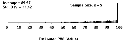
Figure 9b. Histogram illustrating the distribution of estimated PWL values for 1000 simulated lots from a population with 90 PWL, sample 5.
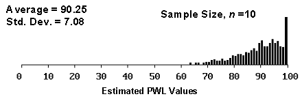
Figure 9c. Histogram illustrating the distribution of estimated PWL values for 100 simulated lots from a population with 90 PWL, sample 10.

Figure 10a. Histogram illustrating the distribution of estimated PWL values for 1000 simulated lots from a population with 70 PWL, sample 3.
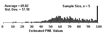
Figure 10b. Histogram illustrating the distribution of estimated PWL values for 1000 simulated lots from a population with 70 PWL, sample 5.
Figure 10c. Histogram illustrating the distribution of estimated PWL values for 1000 simulated lots from a population with 70 PWL, sample 10.
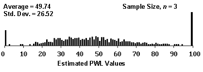
Figure 11a. Histogram illustrating the distribution of estimated PWL values for 1000 simulated lots from a population with 50 PWL, sample 3.
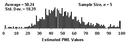
Figure 11b. Histogram illustrating the distribution of estimated PWL values form 1000 simulated lots from a population with 50 PWL, sample 5.
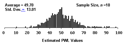
Figure 11c. Histogram illustrating the distribution of estimated PWL values from 1000 simulated lots from a population with 50 PWL, sample 10.
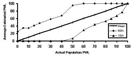
Figure 12a. Illustration 1 of accuracy and precision of PWL estimates.
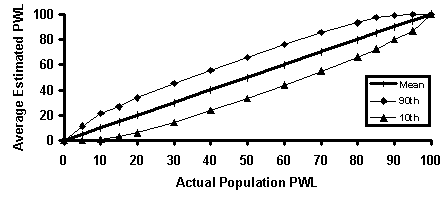
Figure 12b. Illustration 2 of accuracy and precision of PWL estimates.
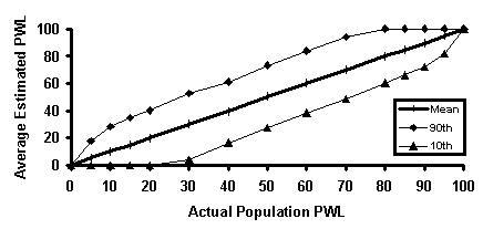
Figure 12c. Illustration 3 of accuracy and precision of PWL estimates.
Table 9. Results of simulation analyses with actual PWL = 90 (distribution of the results from 1000 simulated projects).
| Tests/Lot | Lots/Project | Tests/Project | Avg. Diff. | 2.5% | 97.5% |
|---|---|---|---|---|---|
| 3 | 1 | 3 | +0.1 | -10.0 | +35.0 |
| 3 | 9 | +0.1 | -10.0 | +20.3 | |
| 5 | 15 | -0.3 | -10.0 | +14.3 | |
| 10 | 30 | -0.2 | -9.0 | +9.9 | |
| 20 | 60 | +0.1 | -6.5 | +7.6 | |
| 30 | 90 | -0.0 | -5.1 | +5.9 | |
| 40 | 120 | -0.1 | -4.7 | +4.8 | |
| 50 | 150 | +0.0 | -4.1 | +4.6 | |
| 60 | 180 | -0.1 | -3.6 | +3.9 | |
| 70 | 210 | +0.0 | -3.4 | +3.7 | |
| 80 | 240 | -0.1 | -3.4 | +3.4 | |
| 90 | 270 | -0.0 | -2.9 | +3.1 | |
| 5 | 1 | 5 | -0.2 | -10.0 | +25.5 |
| 3 | 15 | -0.0 | -10.0 | +15.5 | |
| 5 | 25 | +0.0 | -8.3 | +10.5 | |
| 10 | 50 | +0.2 | -6.2 | +7.5 | |
| 20 | 100 | +0.0 | -4.6 | +5.6 | |
| 30 | 150 | +0.1 | -3.8 | +4.2 | |
| 40 | 200 | -0.1 | -3.4 | +3.7 | |
| 50 | 250 | -0.0 | -3.2 | +3.1 | |
| 60 | 300 | +0.0 | -2.8 | +2.8 | |
| 10 | 1 | 10 | +0.1 | -10.0 | +16.6 |
| 3 | 30 | +0.2 | -7.6 | +9.8 | |
| 5 | 50 | +0.0 | -5.7 | +7.2 | |
| 10 | 100 | -0.1 | -4.4 | +4.7 | |
| 20 | 200 | -0.1 | -3.3 | +3.1 | |
| 30 | 300 | +0.1 | -2.7 | +2.9 | |
| 40 | 400 | -0.1 | -2.4 | +2.4 | |
| 50 | 500 | -0.0 | -2.2 | +2.1 |
Avg. Diff. = average difference between the average estimated PWL and the actual PWL for each simulated project
2.5% = value for which 2.5 percent of the simulated average differences were less than or equal
97.5% = value for which 97.5 percent of the simulated average differences were less than or equal
Table 10. Results of simulation analyses with actual PWL = 70 (distribution of the results from 1000 simulated projects).
| Tests/Lot | Lots/Project | Tests/Project | Avg. Diff. | 2.5% | 97.5% |
|---|---|---|---|---|---|
| 3 | 1 | 3 | -1.0 | -30.0 | +44.0 |
| 3 | 9 | +0.3 | -30.0 | +29.6 | |
| 5 | 15 | -0.5 | -20.5 | +21.7 | |
| 10 | 30 | +0.2 | -14.9 | +14.5 | |
| 20 | 60 | -0.0 | -10.3 | +10.8 | |
| 30 | 90 | +0.1 | -8.1 | +8.7 | |
| 40 | 120 | -0.1 | -7.6 | +6.9 | |
| 50 | 150 | -0.1 | -6.7 | +6.4 | |
| 60 | 180 | -0.1 | -5.8 | +6.0 | |
| 70 | 210 | +0.0 | -5.5 | +5.6 | |
| 80 | 240 | +0.2 | -5.0 | +5.5 | |
| 90 | 270 | -0.0 | -4.9 | +5.2 | |
| 5 | 1 | 5 | -0.3 | -30.0 | +34.5 |
| 3 | 15 | -0.1 | -19.2 | +21.7 | |
| 5 | 25 | +0.2 | -15.1 | +16.9 | |
| 10 | 50 | +0.1 | -10.3 | +10.9 | |
| 20 | 100 | -0.1 | -7.7 | +7.6 | |
| 30 | 150 | +0.1 | -6.2 | +6.0 | |
| 40 | 200 | -0.1 | -5.5 | +5.4 | |
| 50 | 250 | +0.2 | -4.8 | +5.4 | |
| 60 | 300 | +0.1 | -4.5 | +4.7 | |
| 10 | 1 | 10 | +0.5 | -22.6 | +27.3 |
| 3 | 30 | +0.2 | -13.5 | +13.7 | |
| 5 | 50 | -0.0 | -10.4 | +10.5 | |
| 10 | 100 | -0.0 | -8.0 | +7.5 | |
| 20 | 200 | -0.0 | -5.3 | +5.1 | |
| 30 | 300 | +0.0 | -4.4 | +4.5 | |
| 40 | 400 | -0.0 | -3.8 | +3.5 | |
| 50 | 500 | +0.0 | -3.2 | +3.4 |
Avg. Diff. = average difference between the average estimated PWL and the actual PWL for each simulated project
2.5% = value for which 2.5 percent of the simulated average differences were less than or equal
7.5% = value for which 97.5 percent of the simulated average differences were less than or equal
Table 11. Results of simulation analyses with actual PWL = 50 (distribution of the results from 1000 simulated projects).
| Tests/Lot | Lots/Project | Tests/Project | Avg. Diff. | 2.5% | 97.5% |
|---|---|---|---|---|---|
| 3 | 1 | 3 | +0.0 | -50.0 | +50.0 |
| 3 | 9 | +0.1 | -31.0 | +29.6 | |
| 5 | 15 | -0.5 | -24.8 | +22.6 | |
| 10 | 30 | -0.2 | -16.3 | +16.2 | |
| 20 | 60 | +0.2 | -12.1 | +11.7 | |
| 30 | 90 | +0.1 | -9.1 | +9.4 | |
| 40 | 120 | +0.0 | -7.7 | +8.3 | |
| 50 | 150 | -0.0 | -6.9 | +7.1 | |
| 60 | 180 | -0.0 | -6.9 | +6.7 | |
| 70 | 210 | -0.0 | -6.0 | +6.0 | |
| 80 | 240 | +0.1 | -5.7 | +6.2 | |
| 90 | 270 | -0.0 | -5.4 | +5.6 | |
| 5 | 1 | 5 | -0.3 | -41.0 | +40.8 |
| 3 | 15 | +0.5 | -21.4 | +20.2 | |
| 5 | 25 | +0.2 | -16.6 | +17.7 | |
| 10 | 50 | -0.2 | -12.2 | +12.5 | |
| 20 | 100 | -0.0 | -8.5 | +8.8 | |
| 30 | 150 | -0.0 | -6.5 | +6.6 | |
| 40 | 200 | +0.0 | -5.7 | +6.0 | |
| 50 | 250 | -0.1 | -5.0 | +5.0 | |
| 60 | 300 | +0.2 | -4.9 | +5.0 | |
| 10 | 1 | 10 | -0.0 | -28.1 | +29.0 |
| 3 | 30 | +0.2 | -15.0 | +14.7 | |
| 5 | 50 | +0.0 | -11.5 | +10.5 | |
| 10 | 100 | +0.2 | -8.1 | +8.2 | |
| 20 | 200 | +0.0 | -5.7 | +5.5 | |
| 30 | 300 | -0.1 | -4.8 | +4.3 | |
| 40 | 400 | -0.0 | -4.1 | +3.9 | |
| 50 | 500 | -0.1 | -3.8 | +3.6 |
Avg. Diff. = average difference between the average estimated PWL and the actual PWL for each simulated project
2.5% = value for which 2.5 percent of the simulated average differences were less than or equal
97.5% = value for which 97.5 percent of the simulated average differences were less than or equal
Figure 13. Plot of average difference of simulated PWL values versus actual PWL values for sample sizes = 3, 5, and 10.
Figure 14a. Plots of the 95th percentile for the average estimated PWL minus the actual PWL at 50 versus the number of lots per project.
Figure 14b. Plots of the 95th percentile for the average estimated PWL minus the actual PWL at 70 versus the number of lots per project.
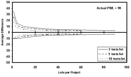
Figure 14c. Plots of the 95th percentile for the average estimated PWL minus the actual PWL at 90 versus the number of lots per project.
For specifications that have a target value, the average deviation from the target value has, in the past, sometimes been used as a means for determining the acceptability of the product. This approach can have the effect of encouraging the contractor to manipulate its process during the production of a lot. For example, if two test results in the morning are below the target value, there is a strong incentive for the contractor to increase the process mean in the afternoon in an effort to get two higher test results so that the average of the four tests for the lot will be near the target value. In essence, this acceptance approach encourages the contractor to increase process variability by making frequent adjustments to the process mean. To avoid the problem of overadjusting the process in response to early test results, the average absolute deviation from the target can be used for the acceptance decision.
The equation for calculating AAD is as follows:
![]() (4)
(4)
where: Xi = individual test results
T = target value
n = number of tests per lot
A computer simulation program was developed to evaluate the accuracy and precision of estimated AAD values. The program generates 1000 simulated lots. The mean, or average, estimated AAD value and the standard deviation for the estimated AAD values are then calculated.
The program can represent populations that are centered on the target value, but can also generate data for populations with means that are offset from the desired target. The actual AAD value for a population centered on the target is 0.798 multiplied by the standard deviation of the population. The actual AAD value increases as the population mean is offset from the target value. Without sacrificing generality, the simulation studies were performed for populations with standard deviation values of 1.00. For a population with a standard deviation other than 1.00, the simulated average AAD values would simply be multiplied by the standard deviation of the population in question.
For the study of AAD accuracy and precision, populations were simulated with offsets from the target that ranged from 0.00 to 2.50 in increments of 0.25. The populations from which the samples were generated were normal distributions with a standard deviation of 1.00.
The shape of the distribution of the sample AAD values varies with the sample size. For small mean offsets, the distribution is skewed to the right, with the degree of skewness determined by the sample size. For a sample size = 1, the peak of the distribution occurs at AAD values near zero. As the sample size increases, the value for the peak of the distribution increases and the degree of skewness decreases, because as the sample size increases, it becomes more and more difficult to have average AAD values near zero. This relationship is shown in table 12.
For a given sample size, the shape of the distribution of the sample AAD values also varies with the offset of the population mean from the target value. The skewness of the distribution stems from the fact that the deviations from the target cannot be below zero, thereby yielding distributions skewed away from zero. As the offset departs farther from the target, the distribution of the sample AAD values approaches symmetry since the deviation values are always greater than zero. This relationship is shown in table 13 for a sample size = 3 and for mean offsets = 0.50 to 2.50.
Table 12. Distributions of sample AAD values for a population centered on the target and for sample sizes = 1, 3, 5, and 10.
| Sample Size, n | Distribution of Sample AAD Values |
|---|---|
| 1 | 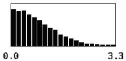 |
| 3 | 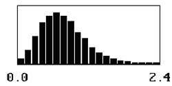 |
| 5 | 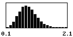 |
| 10 | 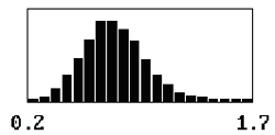 |
Table 13. Distributions of sample AAD values for sample size = 3 and population means offset from the target by 0.50, 1.00, 1.50, 2.00, and 2.50 standard deviations.
| Mean Offset | Distribution of Sample AAD Values |
|---|---|
| 0.50 | 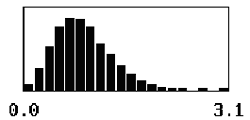 |
| 1.00 | 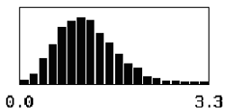 |
| 1.50 | 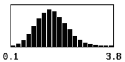 |
| 2.00 | 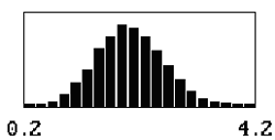 |
| 2.50 | 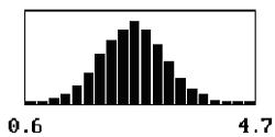 |
Table 14 presents a summary of the simulation results for AAD. The table includes sample sizes = 3, 5, and 10, and populations with means offset from the target by 0.00 to 2.50 standard deviations in increments of 0.25. The table also includes the actual AAD values for each population, which are based on the mean offset values. Finally, the table includes the average differences and the standard deviations for the estimated AAD values.
The results in table 14 show that the sample AAD is an unbiased estimator of the population AAD. It also shows that the standard deviation values decrease as the sample size increases and the standard deviation values increase as the offset from the target value increases. This is caused by the fact that as the offset increases, a deviation value of zero no longer presents a barrier, thereby allowing the deviations to spread evenly on both sides of the AAD value. These two trends are illustrated in figures 15 and 16.
Conceptually, the CI is similar to AAD. While AAD uses the average of the absolute values of the individual deviations from the target value, the CI uses the squares of the individual deviations from the target value. The CI is also similar in concept to the standard deviation. The standard deviation is the root mean square of differences from the mean, whereas the CI is the root mean square of differences from a target. Like AAD, the CI discourages mid-lot process adjustments by not allowing positive and negative deviations from the target to cancel out one another. The CI is calculated as follows:
 (5)
(5)
where: Xi = individual test results
T = target value
n = number of tests per lot
A computer simulation program was developed to evaluate the accuracy and precision of estimated CI values. The program generated 10,000 simulated lots. The mean estimated CI value and the standard deviation for the estimated CI values are then calculated.
The simulation studies present the CI in terms of population standard deviation. Without sacrificing generality, the simulation studies were performed for populations with standard deviations of 1.00. For a population with a standard deviation other than 1.00, the simulated average CI values would simply be multiplied by the standard deviation of the population in question. The program can represent populations that have various CI values. If the population mean is centered on the target, then the CI is the same as the standard deviation. Therefore, the CI cannot be less than zero.
Table 14. Accuracy and precision for AAD estimates (based on the results of 10,000 simulated lots).
| Tests per Lot, n | Offset of Population Mean From Target | Actual AAD of Population | Mean of Estimated AAD Values Minus Actual AAD | Standard Deviation of Estimated AAD Values |
|---|---|---|---|---|
| 3 | 0.00 | 0.798 | -0.003 | 0.3495 |
| 0.25 | 0.823 | +0.002 | 0.3624 | |
| 0.50 | 0.896 | +0.003 | 0.3863 | |
| 0.75 | 1.012 | -0.001 | 0.4223 | |
| 1.00 | 1.167 | +0.005 | 0.4649 | |
| 1.25 | 1.351 | -0.005 | 0.4911 | |
| 1.50 | 1.559 | -0.001 | 0.5200 | |
| 1.75 | 1.782 | +0.008 | 0.5496 | |
| 2.00 | 2.017 | +0.004 | 0.5529 | |
| 2.25 | 2.258 | +0.008 | 0.5660 | |
| 2.50 | 2.504 | +0.003 | 0.5777 | |
| 5 | 0.00 | 0.798 | +0.002 | 0.2717 |
| 0.25 | 0.823 | +0.000 | 0.2758 | |
| 0.50 | 0.896 | +0.002 | 0.2964 | |
| 0.75 | 1.012 | -0.002 | 0.3257 | |
| 1.00 | 1.167 | -0.005 | 0.3575 | |
| 1.25 | 1.351 | +0.004 | 0.3822 | |
| 1.50 | 1.559 | +0.000 | 0.4049 | |
| 1.75 | 1.782 | +0.006 | 0.4216 | |
| 2.00 | 2.017 | +0.002 | 0.4220 | |
| 2.25 | 2.258 | +0.002 | 0.4386 | |
| 2.50 | 2.504 | -0.004 | 0.4425 | |
| 10 | 0.00 | 0.798 | -0.002 | 0.1905 |
| 0.25 | 0.823 | +0.000 | 0.1979 | |
| 0.50 | 0.896 | -0.003 | 0.2101 | |
| 0.75 | 1.012 | +0.003 | 0.2293 | |
| 1.00 | 1.167 | +0.003 | 0.2561 | |
| 1.25 | 1.351 | -0.001 | 0.2693 | |
| 1.50 | 1.559 | -0.002 | 0.2848 | |
| 1.75 | 1.782 | -0.002 | 0.2978 | |
| 2.00 | 2.017 | +0.001 | 0.3033 | |
| 2.25 | 2.258 | -0.003 | 0.3131 | |
| 2.50 | 2.504 | -0.004 | 0.3152 |
Figure 15. Plot of average difference of simulated AAD values versus actual AAD values for sample sizes = 3, 5, and 10.
Figure 16. Plot of how the standard deviation of AAD estimates varies with the population AAD value.
For the study of CI accuracy and precision, populations were simulated with CI values ranging from 1.00 to 3.00. The populations from which the samples were generated were normal distributions with a standard deviation of 1.00.
The shape of the distribution of the sample CI values varies with the sample size in a similar manner to that of AAD. For small CI values, the distribution is skewed to the right, with the degree of skewness determined by the sample size. As the sample size increases, the degree of skewness decreases, because as the sample size increases, it becomes more and more difficult to have average CI values near zero.
Similar to that of AAD, for a given sample size, the shape of the distribution of the sample CI values varies with the CI of the population. For small values of CI, the skewness of the distribution stems from the fact that the squared deviations from the target cannot be below zero, thereby yielding distributions skewed away from zero. As the CI increases, meaning that the population mean is farther from the target, the distribution approaches symmetry since the squared deviation values are always greater than zero.
The results in table 15 show that the sample CI appears to be a slightly biased estimator of the population CI since the average of the CI estimates is always lower than the population CI. This bias decreases as the sample size increases. The table also shows that the standard deviation values decrease as the sample size increases and the standard deviation values increase as the CI value for the population increases. These results are illustrated in figures 17 and 18.
Both the PWL and AAD estimators were unbiased and exhibited similar trends with respect to the variability of their individual estimates. The CI performed essentially the same as AAD, except that it appeared to be a slightly biased estimator. Since the CI offered no benefits compared to AAD and since it appeared slightly biased, it was decided to eliminate the CI and to concentrate further study on only PWL and AAD.
Table 15. Accuracy and precision for CI estimates (based on the results of 10,000 simulated lots).
| Tests per Lot, n | Actual CI of Population | Mean of Estimated CI Values Minus Actual CI | Standard Deviation of Estimated CI Values |
|---|---|---|---|
| 3 | 1.00 | -0.09 | 0.39 |
| 1.10 | -0.07 | 0.43 | |
| 1.25 | -0.10 | 0.44 | |
| 1.40 | -0.07 | 0.41 | |
| 1.50 | -0.08 | 0.49 | |
| 1.75 | -0.08 | 0.52 | |
| 2.00 | -0.07 | 0.54 | |
| 2.25 | -0.05 | 0.53 | |
| 2.50 | -0.05 | 0.56 | |
| 3.00 | -0.05 | 0.56 | |
| 5 | 1.00 | -0.05 | 0.31 |
| 1.10 | -0.05 | 0.34 | |
| 1.25 | -0.04 | 0.37 | |
| 1.40 | -0.06 | 0.38 | |
| 1.50 | -0.08 | 0.39 | |
| 1.75 | -0.02 | 0.39 | |
| 2.00 | -0.06 | 0.43 | |
| 2.25 | -0.01 | 0.43 | |
| 2.50 | -0.04 | 0.44 | |
| 3.00 | -0.03 | 0.44 | |
| 10 | 1.00 | -0.01 | 0.22 |
| 1.10 | -0.03 | 0.24 | |
| 1.25 | -0.03 | 0.27 | |
| 1.40 | -0.03 | 0.27 | |
| 1.50 | -0.03 | 0.27 | |
| 1.75 | -0.02 | 0.29 | |
| 2.00 | -0.02 | 0.30 | |
| 2.25 | -0.01 | 0.31 | |
| 2.50 | 0.00 | 0.30 | |
| 3.00 | -0.02 | 0.30 |
Figure 17. Plot of average difference of simulated CI values versus actual CI values for sample sizes = 3, 5, and 10.
Figure 18. Plot of how the standard deviation of CI estimates varies with the population CI value.