U.S. Department of Transportation
Federal Highway Administration
1200 New Jersey Avenue, SE
Washington, DC 20590
202-366-4000
Federal Highway Administration Research and Technology
Coordinating, Developing, and Delivering Highway Transportation Innovations
| REPORT |
| This report is an archived publication and may contain dated technical, contact, and link information |
|
| Publication Number: FHWA-HRT-14-023 Date: May 2014 |
Publication Number: FHWA-HRT-14-023 Date: May 2014 |
In order to obtain the bridge wire corrosion rate from LPR sensors, a relationship between corrosion rate and Rp readings from the sensors is needed. The corrosion rate is calculated from Rp and mass loss measurements on the corroding metal using the concept of equivalent weight and Faraday's Law. Equivalent weight (EW) is the amount of an element that reacts with 1 Faraday of charge, thus contributing to the corrosion and overall loss of material in the basic oxidation process for metals:M→Mz+ + ze-. Here Mindicates a metal atom, e indicates electron and z is the number of electrons lost per atom of meta. EW is calculated from the known atomic weight (AW) of the metal and z as follows:
![]()
Figure 214. Equation. Equivalent weight
In order to relate the mass loss of metal to the current flow, Faraday's law is stated as follows:
![]()
Figure 215. Equation. Relationship between the charge from the corrosion reaction with
the number of lost electron and the moles of metal
Where:
Q = Charge in Coulombs resulting from the reaction of corroding metal
F = Faraday's constant (i.e., 96,485.34 Coulombs/mole).
z = Number of electrons lost per atom of the metal.
M = Number of moles of metal reacting.
For the number of moles lost for the metal M, the amount of mass loss W can be calculated as follows:
![]()
Figure 216. Equation. Amount of mass loss
Combining figure 214 through figure 216 and substituting for z and M, W can be related to charge Q as follows:
![]()
Figure 217. Equation. Relationship between the amount of mass loss with the equivalent
weight and the charge
W can be converted to corrosion rate from the density and sampling area of the corroding metal using the basic identities as follows:
![]()
Figure 218. Equation. Mass loss related to density of the material and volume of the lost
material
![]()
Figure 219. Equation. Charge as the product of the corrosion current and time
Where:
ρ = Density of metal.
V = Volume of corroding metal corresponding to the sampling area.
A = Sampling area.
T = Thickness of corrosion layer corresponding to the sampling area.
Icorr = Corrosion current.
t = Time in seconds.
From figure 219, the following can be obtained:
![]()
Figure 220. Equation. Mass loss from geometric considerations to the mass loss from
equivalent weight and charge
![]()
Figure 221. Equation. Rate of change of thickness
The rate of change of thickness ![]() is the corrosion rate (CR) of the metal as follows:
is the corrosion rate (CR) of the metal as follows:
![]()
Figure 222. Equation. Corrosion rate of the metal
Where K is a constant that accounts for Faraday's constant (F) in figure 221 and changes units of corrosion from seconds to years. Icorrcan be substituted to yield the following:
![]()
Figure 223. Equation. Alternative expression of the corrosion rate
![]()
Figure 224. Equation. Simplified expression of the corrosion rate
Where B' is the overall proportionality constant in units mm-ohms/year. In order to determine B', LPR sensors and ungalvanized bridge wires were tested together in various cyclic corrosion tests.
From the mass loss experiments with actual bridge wires, researchers determined the corrosion loss for each test. Both recorded Rp values and corrosion mass loss values were used to estimate the overall proportionality constant B' in figure 224.
The sampling frequency for Rp during the corrosion test was 1 recording/min. Hence, the estimated thickness loss induced by corrosion during a given minute (C 1-min) can be obtained by converting the corrosion rate CR in inches/year (mm/year) to inches/min (mm/min) and then multiplying times 1 min as follows:

Figure 225. Equation. Estimated thickness loss in 1 min
Substituting for CR the expression presented in figure 224 leads to an expression for the thickness loss during a given minute as follows:

Figure 226. Equation. Alternative expression of the estimated thickness loss in 1 min
Where Rp is obtained directly from the measurements. The total thickness loss for the duration of 3 (h) x 60 (min) x 48 (cycle) = 8,640-min experiments (C Exp) will then be expressed as follows:

Figure 227. Equation. Expression of the estimate of the total thickness loss
Where the summation is intended for all the values recorded during the experiment. In this case, the proportionality constant B' can then be obtained from the following:

Figure 228. Equation. Proportionality constant as function of the thickness loss and of the polarization resistance
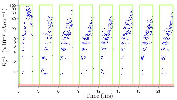
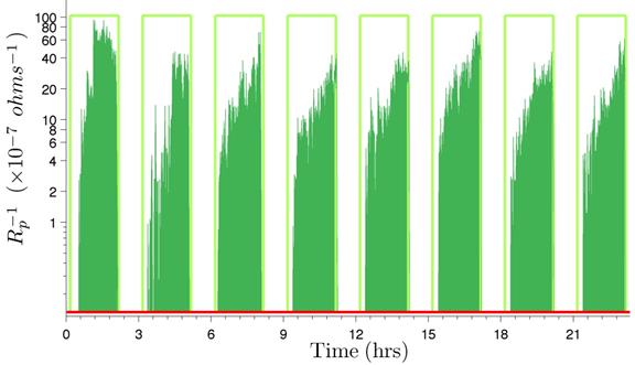
As an example, the calculation of B' for the 0.006-inch (150-µm) LPR sensor used in experiment 1 is provided. In this experiment, only one 0.006-inch (150-µm) LPR sensor was placed in the chamber with the wires. Figure 229 shows the inverse of Rp readings for this sensor during the first eight cycles of experiment 1. Each data point on the plot corresponds to the inverse of Rp at a given instant in time and is proportional to the instantaneous corrosion rate value at that recording time, following the relation given by figure 226. The integration of this time series (multiplication of these values by the sampling interval (1 min) and summation of all these products) yields the denominator of figure 227.
The integrated area is shown for the first eight cycles of experiment 1 in figure 230. The area for the entire duration of the test (its integration) is 7.1020 x 10⁻³ min/ohms.

Figure 229. Graph. Inverse of Rp versus time

Figure 230. Graph. Integration of inverse of Rp
The average thickness loss measured for the ten specimens tested in experiment 1 is 0.0006 inch (14.87 µm). This is obtained by measuring the wires before and after the experiment, as previously described. Overall proportionality constant B' for the sensor can then be calculated as follows:

Figure 231. Equation. Estimation of constant of proportionality from experiment 1
Where:
 = 7.1020 * 10-3 (min/ohms).
CExp-1 = 0.0006 inch (14.87 µm).
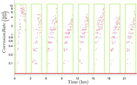
Hence, when using measurements from the 0.006-inch (150-µm) LPR sensors, dividing this value of B' by Rp will provide an instantaneous measurement of the corrosion rate of the wire. Figure 232 displays the instantaneous corrosion rate values calculated using the overall proportionality constant B'.

1 inch = 25.4 mm
Figure 232. Graph. Instantaneous corrosion rates versus time