Active Traffic Management: Comprehension, Legibility, Distance, and Motorist Behavior in Response to Selected Variable Speed Limit and Lane Control Signing

Chapter 4. Driver DecisionMaking

This study used a driving simulator to examine driver decisionmaking in a dynamic environment. The study employed the same scenarios that were used in the laboratory study (see chapter 2). The focus of this study was to examine drivers' responses (behavioral and eye-gaze movements) and compliance with LCSs and VSL signs. This experiment used roadway structures similar to those in the Washington deployment. Specific signs were selected based on the laboratory and field test results (see chapter 3) and included signs with designs similar to those in both the Washington and Minnesota deployments.

Methods

The Simulator

The simulator's screen consists of a 240-degree portion of a cylinder with a radius of 8.9 ft (2.7m). Directly in front of the driver, the design eye point of the simulator was 9.5 ft (2.9 m) from the screen. The stimuli were projected onto the screen by five Barco projectors with resolution of 2,048 horizontal by 1,536 vertical pixels. Participants sat in a late model compact sedan as shown in figure 42. The simulator's motion base was not enabled in this experiment. The car's instrument panel, steering, brake, and accelerator pedal all functioned in a manner similar to real-world compact cars.

Figure 42. Photo. The FHWA Highway Driving Simulator.

The simulated vehicle was equipped with a hidden intercom system that enabled communications between the participant and a researcher who ran the experiment from a control room. The researcher in the control room could also view the face video from the eye-tracking system and thereby monitor the participant's wellbeing.

ATM Signs

Figure 43 through figure 49 depict the ATM signs used in this experiment. In addition, the leftmost CMS occasionally displayed HOV2 restriction information. These signs represent a selection of signs that were being used in ATM test deployments in Washington and Minnesota at the time of this study. Selection of these signs was based on the results of sign comprehension and preference testing done in a laboratory setting (see chapter 2).

Figure 43. Graphic. Lane open (fully operational) option used in first simulator study.

Figure 44. Graphic. Lane closed option used in first simulator study.

Figure 45. Graphic. Lane closed ahead with legend option used in first simulator study.

Figure 46. Graphic. Merge right with legend option used in first simulator study with streaming chevrons).

Figure 47. Graphic. Merge left with legend option used in first simulator study with chevrons streaming.

Figure 48. Graphic. Merge left or right with legend option used in first simulator study with chevrons streaming.

Figure 49. Graphic. VSL sign used in first simulator study.

Because the Washington roadway structure design was used, side-mounted CMSs were present. The following messages were displayed on the side-mounted CMSs, depending on which scenario the participant was currently experiencing: (1) STALLED VEHICLE AHEAD, (2)CENTER LANE CLOSED, (3) ACCIDENT AHEAD MERGE RIGHT, (5) RIGHT LANES CLOSED, (6) RIGHT LANES EXIT ONLY, (7) REDUCE SPEED ZONE AHEAD, (8)REDUCE SPEED ZONE, and (9) END REDUCE SPEED ZONE.

Simulation Scenarios

The participants drove on a simulated eight-lane highway (four lanes in each direction of travel) approximately 23 mi (37.0 km) in length. A 1-mi (1.61-km) section of freeway without overhead signs preceded the first overhead ATM sign. The ATM signs (gantries) were spaced every 0.5 mi (0.8 km) along the roadway. Because of limitations in the resolution of the simulator's projectors, all signs in the simulator were oversized so that their legibility distance approximated real-world legibility distances. In this experiment, signs were twice the size of their real-world equivalent. Figure 50 shows an example of an ATM sign at the start of an area requiring a slowdown in speed.

Figure 50. Screen capture. ATM sign warning of a reduced speed zone ahead.

Each drive was composed of the following scenarios:

1. Resting condition for the signs (normal operations for all lanes).
2. Stalled vehicle closing 1 lane (right-center lane—lane 3).
3. Vehicle crash closing two left lanes (lanes 1 and 2).
4. Vehicle crash closing two right lanes (lanes 3 and 4 with exit ramp open).
5. Message in the event of slow-moving traffic in all lanes (speed reduction).

A resting condition for the signs was used between the other scenarios in the study. Figure 51 shows the ATM sign configuration for the resting condition. Three signs at 0.5-mi (0.8-km) intervals were used for the resting condition. Figure 52 through figure 55 show the configurations of the ATM signs for the other scenarios in the study. With the exception of the resting condition, all of the other scenarios included six ATM signs spaced 0.5 mi (0.8 km) apart.

Figure 51. Illustration. Design of scenario 1—resting condition for ATM signs (normal operations for all lanes).

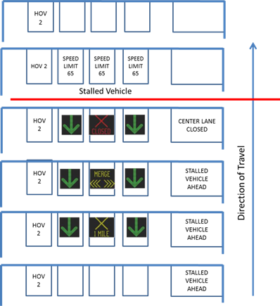
Figure 52. Illustration. Design of scenario 2—stalled vehicle design closing 1 lane (right-center lane—lane 3).

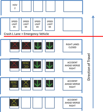
Figure 53. Illustration. Design of scenario 3—vehicle crash scenario design closing two left lanes (lanes 1 and 2).

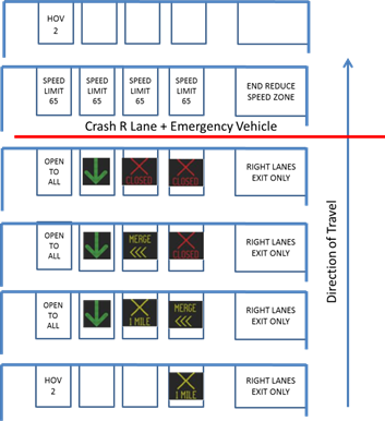
Figure 54. Illustration. Design of scenario 4—Vehicle crash scenario design closing two right lanes (lanes 3 and 4 with exit ramp open).

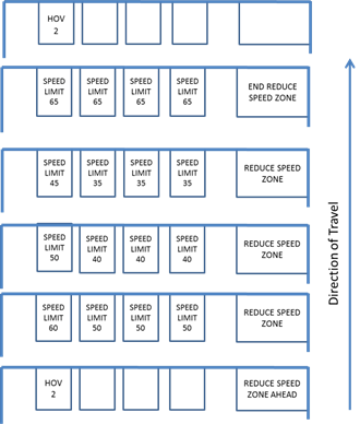
Figure 55. Illustration. Design of scenario 5—slow-moving traffic in all lanes.

The scenarios illustrated in figure 51 through figure 55 were combined to generate a simulated drive (see table 14 for an example). For the experiment, four orders were created from the scenarios using partial counterbalancing. Participants were instructed to exit at Holt Ave, which was always located at the end of the drive during the two right lanes closed scenario. Also, the reduced speed scenario was presented twice during each of the drives. Table 15 presents the fourorders of the scenarios used in the experiment. There were eight participants for each of the four driving orders.

Table 14. Sample ordering of scenarios to create a simulated drive.

1 mi = 1.61 km.
— Indicates not applicable.

Table 15. Four orders of scenarios within simulated drives.

1 mi = 1.61 km.

To make the driving task more realistic and visually demanding, vehicle traffic was simulated. The Vissim™ traffic model was used to generate the behavior of vehicles in the traffic stream.⁽¹²⁾ Because the random number seed for the traffic model was always the same, all participants were immersed in the same traffic stream. However, because the participants controlled their own speed, acceleration, and lane choice, they could experience different traffic conditions in their immediate surroundings.

At the beginning of test sessions, 5,000 veh/h (1,250 veh/h per lane) were generated for 6.7 min. Participants were instructed to begin driving 2.5 min into this period of traffic generation. Approximately every 3 mi (4.8 km), 500 veh/h would exit the freeway at off ramps, and 500veh/h would merge into the traffic stream from on ramps. There were off and on ramps every 1.5 mi (2.4 km), although the traffic model populated only half of these ramps with traffic.

Participants were instructed to maintain 65 mi/h (105 km/h) and to drive in the second lane from the right, except when they wanted to pass. This instruction resulted in most participants staying within the initially generated traffic flow throughout the experiment.

A short practice session preceded the test session. The original purpose of the practice session was to enable the participants to become accustomed to the handling characteristics of the simulated vehicle. However, pilot testing showed that some participants thought they were supposed to stay on the freeway, regardless of ATM sign warnings or guide signs. Therefore, the training session was modified to ensure that participants knew it was expected they should follow instructions on the ATM signs. The modified training included a side-mounted CMS that instructed participants to take the next exit.

Eye-Tracking System

The simulator was equipped with a Smart Eye® four-camera dashboard-mounted eye-tracking system that sampled at 120 Hz.⁽¹³⁾ The system tracked horizontal gaze direction from approximately the location of the right outside mirror to the left outside mirror, and vertical gaze direction from the instrument panel to the top of the windscreen. Gaze direction accuracy varied by participant. The mean accuracy of gaze position across participants was 1.36 degrees (radius) with a 0.54-degree STD. The eye-tracking data (i.e., gaze direction of each eye, head position, etc.) were merged with data from the simulator (e.g., vehicle speed, lane position, steering wheel position) and the current forward view of the simulation visual scene (approximately 60 degrees horizontal by 40 degrees vertical). The merge was accomplished using a MAPPS™ scene recorder.⁽¹⁴⁾

To quantify when and for how long participants looked at each ATM sign, a researcher used analysis software to indicate a region of interest (ROI) on individual frames of the recorded video image. An example of an ROI is shown in figure 56 (the halo around the signs). ROIs were created between the point a sign began to pass out of the driver's view and 10 s upstream of that point. Two ROIs were created for the ATM signs: (1) ATM_LEFT, which encompassed the four per-lane CMSs; and (2) ATM_RIGHT, which encompassed the side-mounted CMS. An ROI for the road ahead (RA) was also created. The ROIs for this study are shown in figure 56.

Figure 56. Screen capture. ROIs indicated on the ATM signs.

Participants

Thirty-one participants (15 males and 16 females) completed the study. All were licensed drivers from the Washington, DC, metropolitan area. The mean age of participants was 47 years old (range 21 to 72 years old). Of these 31 participants, 27 provided interpretable eye-tracking data. Useable behavioral data were obtained from four participants for whom eye-tracking was unsuccessful. The mean age of the 27 participants (13 males and 14 females) with good eye-tracking data was 45 years old (range 21 to 72 years old). Only one participant reported a mild simulator sickness symptom (headache), and no participant dropped out as a result of simulator sickness.

Results

In all the figures pesented in this section (figure 83 through figure 86), error bars indicate 95-percent confidence limits. Also, for ease of understanding, the scenarios were coded in the figures as follows (there are two codes for scenario 5 (speed reduction) because participants viewed this scenario twice):

1. REST: Resting condition for the signs (normal operations for all lanes).
   
   
2. SVRCX: Stalled vehicle closing 1 lane (right-center lane—lane 3).
   
   
3. 2LFTX: Vehicle crash closing two left lanes (lanes 1 and 2).
   
   
4. 2RTXE: Vehicle crash closing two right lanes (lanes 3 and 4 with exit ramp open).
   
   
5. SLOW1/SLOW2: Message in the event of slow-moving traffic in all lanes (reduced speed).

The last scenario for all participants included the Holt Ave exit. The participants were informed at the start of the drive to exit the freeway when they came to the Holt Ave exit. After the data collection runs began, researchers noticed that there were only two guide signs for the Holt Ave exit (one advanced guide sign 1 mi (1.61 km) before the exit—HOLT3—and one guide sign at the exit—HOLT1) and a second advanced guide sign 0.5 mi (0.8 km) before the exit (HOLT2) had not been included. After seven participants had completed the experiment, the second advanced guide sign (at 0.5 mi (0.8 km)) was added to the scenario. The first set of analyses compared the exiting behavior of the participants that did not have the 0.5 mi (0.8 km) exit sign with those that did. This analysis was of an exploratory nature given the small sample size for the participants without the 0.5 mi (0.8 km) sign.

Inclusion of Half-Mile Advance Guide Sign

Exit-Taking Behavior

This analysis compared the exit-taking behavior of those participants who were presented with the second advanced guide sign to those participants who were not. First, all participants who completed the study (N = 31) were included in the final dataset. Seven participants were not presented with the second advanced guide sign and 24 were. Table 16 shows the relationship (row percentages) between inclusion of the second advanced guide sign and exit-taking behavior. Chi-squared test results indicated that there was no significant association between the presence of the second advanced guide sign and exit-taking behavior.

Table 16. Distribution (row percentages) of inclusion of the second advanced guide sign by exit-taking behavior for all subjects (N = 31).

Next, only those participants who had reasonable eye-tracking data (N = 27) were included in the final dataset. There were 5 participants who were not presented with the second advanced guide sign and 22 that did. As shown in table 17, the results were similar as in the first analysis. Again, Chi-squared test results indicated that there was no significant association between the presence of the second sign and exit-taking behavior.

Table 17. Distribution (row percentages) of inclusion of the second exit sequence sign by exit-taking behavior for only subjects with reasonable eye-tracking data (N = 27).

Eye-Tracking Behavior

A glance toward an ROI was defined as when a participant registered 12 or more hits (where a hit was defined as one 120-Hz gaze point on an ROI) toward the ROI during a data collection zone (DCZ). For this analysis, each of the three exit signs (HOLT3, HOLT2, and HOLT1) was considered individually. In other words, drivers who were presented with the second advanced guide sign (HOLT2) could have a maximum of three glances during the last scenario, where participants were tasked to exit at Holt Ave (two right lanes blocked); those drivers who were not presented with the second sign could have a maximum of two glances. By this design, if participants dedicated the same amount of attention to each of the signs in the exit sequence, then those drivers who were presented with the second sign (HOLT2) should exhibit a higher probability of glancing than those drivers who were not. Results from a repeated measures logistic regression supported this claim—there was a statistically significant difference in the probability of glancing between the two groups (χ² (2) = 4.80, p < 0.05). Figure 57 shows the predicted mean probability of glancing toward an exit sign by driver group.

Figure 57. Graph. Predicted mean probability of glancing at an exit sign by inclusion of HOLT2 sign.

Lane Choice Behavior

By Researcher Observation

During data collection, researchers observed a participant's lane position following each gantry in the scenario. In scenario 1 (resting condition), four observations were recorded, one for each gantry. This scenario was presented to each participant at the beginning of the drive and then in between each of the other scenarios. Table 18 shows the distribution (row percentages) of lane choice across participants for each recorded observation. Chi-squared test results indicated that there was no significant association between the observation in the scenario and lane choice. Overall, participants tended to stay in lane 3 (the right-center lane) as initially instructed by the researcher.

Table 18. Distribution (row percentages) of lane choice by observation for scenario1 (resting condition).

— Indicates 0 percent.

In scenario 2 (stalled vehicle ahead), six observations were recorded, one for each of the fivegantries and one for the stalled vehicle between the fourth and fifth gantries. Table 19 shows the distribution (row percentages) of lane choice for each recorded observation. Chi-squared test results indicated that there was a significant association between the observation in the scenario and lane choice (χ² (10) = 108.33, p < 0.001). The data indicate that participants exited lane 3 in accordance with the instructions on the ATM signs; however, most of the participants exited lane3 before being shown the sign indicating they should merge out of the lane. After the stalled vehicle was passed, participants reentered lane 3. No participant crashed with the stalled vehicle in lane 3.

Table 19. Distribution (row percentages) of lane choice by observation for scenario 2 (stalled vehicle ahead).

— Indicates 0 percent.

Figure 58 shows the speed profile for this scenario. The participants slowed down about 5 mi/h (8 km/h) on average when encountering the CMS indicating a stalled vehicle ahead. On average, the participants did not deviate much from the posted speed limit, although they did make the necessary lane changes.

1 mi/h = 1.61 km/h.
1 ft = 0.305 m.

Figure 58. Graph. Speed profile for scenario 2 (stalled vehicle ahead).

In scenario 3 (two left lanes closed owing to a crash), six observations were recorded, one for each of the five gantries and one for the crash between the fourth and fifth gantries. Table 20 shows the distribution (row percentages) of lane choice for each recorded observation. Chi-squared test results indicated there was no significant association between the observation in the scenario and lane choice. Compared with scenario 1, there was a shift of traffic into lane 4. The speed profile for this scenario (not pictured) was similar to that observed in scenario 2 (see figure 58).

Table 20. Distribution (row percentages) of lane choice by observation for scenario 3 (twoleft lanes closed).

— Indicates 0 percent.

In scenario 4 (two rights lanes closed owing to a crash), three observations were recorded, onefor each of the three gantries. Table 21 shows the distribution (row percentages) of lane choice for each recorded observation. Chi-squared test results indicated that there was a significant association between the observation in the scenario and lane choice (χ² (4) = 40.20, p < 0.001). This was a challenging scenario in which the two right lanes were closed, but the rightmost lane (lane 4) was still open for exiting. However, the majority (74 percent) of the participants successfully exited at Holt Ave in accordance with instructions.

Table 21. Distribution (row percentages) of lane choice by observation for scenario 4 (two right lanes closed).

— Indicates 0 percent.

Figure 59 shows the speed profile for this scenario. On average, the participants slowed a few miles per hour (less than 5 mi/h (8 km/h)) until they approached the exit and then significantly decreased their speeds (more than 10 mi/h (16 km/h)) when they began to exit.

1 mi/h = 1.61 km/h.
1 ft = 0.305 m.

Figure 59. Graph. Speed profile for scenario 4 (two right lanes closed).

In scenario 5 (speed reduction), five observations were recorded, one for each of the fivegantries. This scenario was presented to each participant two times (scenarios 5a and 5b). Table 22 below shows the distribution (row percentages) of lane choice for each recorded observation. Both presentations (scenarios 5a and 5b) resulted in the same distribution; thus, only one table is included. Chi-squared test results indicated there was no significant association between the observation in the scenario and lane choice.

Table 22. Distribution (row percentages) of lane choice by observation for each presentation of scenario 5.

— Indicates 0 percent.

Figure 60 presents the speed profile for the first presentation of scenario 5 (speed reduction). In this scenario, the participants were informed on the side-mounted CMS that there was slow traffic ahead. The VSL signs showed lower speed limits every 0.5 mile (0.8 km). On average, the participants followed the VSL signs.

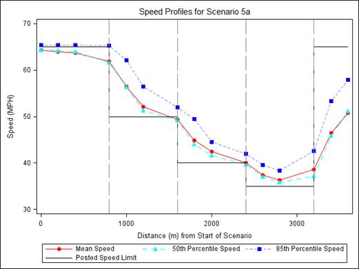
1 mi/h = 1.61 km/h.
1 ft = 0.305 m.

Figure 60. Graph. Speed profile for scenario 5a (first speed reduction).

Lane Choice Compliance

Only data from scenario 2 (stalled vehicle ahead) and scenario 3 (two left lanes closed owing to crash) were reviewed to determine lane choice compliance. DCZs started approximately 1,000 ft (304.8 m) prior to the gantry and ended 880 ft (268.2 m) after the gantry. Given that gantries were placed 0.5 mi (0.8 km) apart, the ending location of the DCZ was one-third of the distance to the subsequent gantry. Lane position for the last frame of each DCZ was kept for the final dataset. Table 23 and table 24 show the distribution (row percentages) of lane choice by DCZ for scenario 2 and scenario 3, respectively. Data for scenario 2 suggest that participants exited lane 3 in accordance with the instructions on the ATM signs. Once the stalled vehicle was encountered, participants reentered lane 3. During scenario 3, participants tended to stay out of the blocked lanes (lanes1 and 2).

Table 23. Distribution (row percentages) of lane choice by DCZ for scenario 2 (stalled vehicle ahead).

— Indicates 0 percent.

Table 24. Distribution (row percentages) of lane choice by DCZ for scenario3 (two left lanes closed).

— Indicates 0 percent.

Speed Behavior

In the following sections, only the two occurrences of scenario 5 (speed reduction scenario; scenarios 5a and 5b) were reviewed because this was the only scenario that directed participants to vary their speed. DCZs started approximately 1,000 ft (304.8 m) prior to the gantry and ended 880 ft (268.2 m) after the gantry. Given that gantries were placed 0.5 mi (0.8km) apart, the ending location of the DCZ was one-third of the distance to the subsequent gantry.

Speed Compliance

Data were reviewed to determine whether a participant was compliant at least once during a DCZ. If a participant became compliant multiple times during a DCZ, then only the last point of compliance was kept for analysis. Chi-squared tests were performed to determine whether compliance varied among the five DCZs encountered during scenario 5. When considering only scenario 5a, results indicated there was a significant difference between the five DCZs (χ² (4) = 20.70, p < 0.001). The greatest deviation from the expected frequency occurred during the fifth DCZ in which no participants were compliant with the posted speed limit of 65 mi/h (105 km/h). Table 25 shows the distribution of speed compliance for each DCZ.

Table 25. Distribution (row percentages) of speed compliance by DCZ for the scenario 5a (first speed reduction).

— Indicates 0 percent.

Similarly, when considering only scenario 5b, results indicated there was a significant difference in speed compliance among the five DCZs (χ² (4) = 22.87, p < 0.001). Once again, the greatest deviation from the expected frequency occurred during the fifth DCZ; only one participant was compliant with the posted speed limit of 65 mi/h (105 km/h). Table 26 shows the distribution of speed compliance for each DCZ.

Table 26. Distribution (row percentages) of speed compliance by DCZ for scenario 5b (second speed reduction).

— Indicates 0 percent.

Distance of Speed Compliance

Data were reviewed to determine whether a participant was compliant at least once during a DCZ. If a participant was compliant more than once during a DCZ, then only the last point was kept for analysis. The distance (in meters) from the gantry at which the participant became compliant was calculated. Positive values indicated that the participant became compliant before the gantry, and negative values indicated that compliance occurred after the gantry. Only one DCZ (the first DCZ for scenario 5b) resulted in a positive average distance for the location of compliance. Table 27 and table 28 show the summary statistics of location of speed compliance for scenario 5a and scenario 5b, respectively.

Table 27. Summary statistics for the location of speed compliance relative to the gantry by DCZ for scenario 5a (first speed reduction).

3.28 ft = 1 m.
— Indicates non-calculable values.

Table 28. Summary statistics for the location of speed compliance relative to the gantry by DCZ for scenario 5b (second speed reduction).

3.28 ft = 1 m.
— Indicates non-calculable values.

Glance Behavior

A glance toward an ROI was defined as when a participant registered 12 or more hits toward the ROI during a DCZ. If a glance occurred, then the number of hits was multiplied by 120 (the advertised sampling rate of the eye-tracking system) to calculate the duration.

Glance Probability

Repeated measures logistic regression was used to determine whether there was a difference in the probability of a glance across the different scenarios. Recall that scenario 5 (speed reduction) was viewed twice by each participant (scenario 5a and scenario 5b, respectively). However, data from each viewing was kept separate and analyzed as two independent scenarios.

When considering only the overhead ATM signs (ATM_LEFT), results indicated there was a statistically significant difference in the probability of a glance between the different scenarios (χ² (4) = 30.44, p < 0.001). As is shown in figure 61, scenario 5a (first speed reduction) yielded the largest probability of a glance, and scenario 4 (two right lanes blocked, take exit) yielded the smallest probability.

Figure 61. Graph. Predicted mean probability of glancing at ATM_LEFT by scenario.

When considering only the larger side-mounted CMS (ATM_RIGHT), results indicated there was a statistically significant difference in the probability of a glance between the different scenarios (χ²(4) = 26.14, p < 0.001). As is shown in figure 62, scenario 5a (first speed reduction) yielded the largest probability of a glance, and scenario 4 (two right lanes blocked, take exit) yielded the smallest probability.

Figure 62. Graph. Predicted mean probability of glancing at ATM_RIGHT by scenario.

Glance Duration

General estimating equations (GEEs) with a Gamma response distribution and identity link function were used to analyze the duration of a glance, given that a glance had occurred. In other words, no durations of 0 s were included in the analysis.

When considering only glances to ATM_LEFT, results indicated that there was a statistically significant difference in the duration of a glance between the scenarios (χ² (4) = 13.34, p = 0.010). As is shown in figure 63, scenario 4 (two right lanes blocked, take exit) yielded the longest glance duration, and scenario 3 (two left lanes closed) yielded the shortest.

Figure 63. Graph. Predicted mean glance duration at ATM_LEFT by scenario.

When considering only glances to ATM_RIGHT, results indicated that there was no statistically significant difference in the duration of a glance between the scenarios. Overall, the mean glance duration was about 0.59 s. Figure 64 below shows the predicted mean glance duration by scenario.

Figure 64. Graph. Predicted mean glance duration at ATM_RIGHT by scenario.

Look Behavior

A look was defined as any accumulation of 7 or more hits on an ROI within a series of 12 frames (100 ms). A look began when this criterion was first met and terminated when the number of hits within the preceding 12 frames dropped below 7.

Look Probability

Repeated measures logistic regression was used to determine whether there was a difference in the probability of at least one look across the different scenarios. Recall that scenario 5 (speed reduction) was viewed twice by each participant. However, data from each viewing was kept separate and analyzed as two independent scenarios (scenario 5a and 5b, respectively).

When considering only the overhead ATM signs (ATM_LEFT), results indicated there was no statistically significant difference in the probability of at least one look between the different scenarios. Overall, this probability was about 0.52. Figure 65 shows the probability of at least one look for each of the scenarios.

Figure 65. Graph. Predicted mean probability of at least one look at ATM_LEFT by scenario.

When considering only looks to ATM_RIGHT, results indicated there was no significant difference in the probability of at least one look between the different scenarios. Overall, this probability was about 0.44. Figure 66 shows the probability of at least one look for each of the scenarios.

Figure 66. Graph. Predicted mean probability of at least one look at ATM_RIGHT by scenario.

Number of Looks

Repeated measures Poisson regression was used to determine whether the number of looks (assuming at least one look occurred) among between the different scenarios. Recall that scenario5 (speed reduction) was viewed twice by each participant. However, data from each viewing was kept separate and analyzed as two independent scenarios (scenario 5a and 5b, respectively).

When considering only the overhead ATM signs (ATM_LEFT), results indicated there was a statistically significant difference in the number of looks across the scenarios (χ² (4) = 28.94, p < 0.001). Figure 67 shows the predicted mean number of looks by scenario. Despite having only three ATM signs (as opposed to five as in the other scenarios), scenario 4 (two right lanes blocked, take exit) resulted in the greatest number of looks. Scenario 5b (second speed reduction) yielded the fewest.

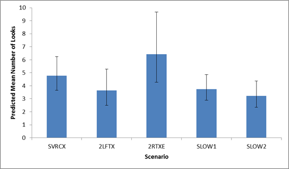
Figure 67. Graph. Predicted mean number of looks at ATM_LEFT by scenario.

When considering only ATM_RIGHT, results indicated there was a statistically significant difference in the number of looks across the scenarios (χ² (4) = 12.22, p = 0.016). There were generally fewer looks toward ATM_RIGHT than toward ATM_LEFT. However, the greatest number of looks to ATM_RIGHT was still in scenario 4 (two right lanes blocked, take exit; see figure 68). The fewest number of looks occurred during scenario 5b (second speed reduction).

Figure 68. Graph. Predicted mean number of looks at ATM_RIGHT by scenario.

Look Duration

GEEs with a Gamma response distribution and identity link function were used to determine whether the duration of looks (assuming at least one look occurred) varied among the different scenarios. Recall that scenario 5 (speed reduction) was viewed twice by each participant. However, data from each viewing was kept separate and analyzed as two independent scenarios (scenario 5a and 5b, respectively).

When considering only the overhead ATM signs (ATM_LEFT), results indicated there was no statistically significant difference in the duration of looks across the scenarios. Overall, the mean look duration was 0.14 s. Figure 69 shows the predicted mean look duration for each scenario.

Figure 69. Graph. Predicted mean look duration at ATM_LEFT by scenario.

When considering only ATM_RIGHT, results indicated there was a statistically significant difference in look duration between the different scenarios (χ²(4) = 12.34, p = 0.015). Figure 70 shows the predicted mean look duration for each scenario. Although scenario 5b (second speed reduction) yielded the fewest looks to ATM_RIGHT (see figure 68), these looks were the longest in duration. Scenario 2 (stalled vehicle) resulted in the shortest look durations.

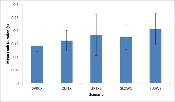
Figure70. Graph. Predicted mean look duration at ATM_RIGHT by scenario.

Fixation Behavior

A fixation was defined as seven consecutive gaze positions (60 ms) within a fixation radius of 4 percent of the vertical image height (i.e., 15 pixels on the 372-pixel image) and centered on the first of the seven gaze positions that designated the start of a fixation. The fixation continued until there were six consecutive hits (50 ms) outside the fixation radius. For a simulated object 500 ft (152 m) ahead, the fixation radius subtended a visual angle of about 2 degrees. A fixation on an ROI was recorded if the center of the fixation was on the ROI.

Fixation Probability

Repeated measures logistic regression was used to determine whether there was a difference in the probability of at least one fixation across the different scenarios. Recall that scenario 5 (speed reduction) was viewed twice by each participant. However, data from each viewing was kept separate and analyzed as two independent scenarios (scenario 5a and 5b, respectively).

When considering only the overhead ATM signs (ATM_LEFT), results indicated there was a statistically significant difference in the probability of at least one fixation between the different scenarios (χ² (4) = 13.46, p = 0.009). Figure 71 shows the probability of at least one fixation for each of the scenarios. Scenario 2 (stalled vehicle) and scenario 5b (second speed reduction) resulted in the highest probability of at least one fixation, while scenario 3 (two left lanes closed) yielded the lowest corresponding probability.

Figure 71. Graph. Predicted mean probability of at least one fixation on ATM_LEFT by scenario.

When considering only fixations to ATM_RIGHT, results indicated there was a statistically significant difference in the probability of at least one fixation between the different scenarios (χ² (4) = 13.02, p = 0.011). Figure 72 shows the probability of at least one fixation for each of the scenarios. Overall, this probability was less than the corresponding probability for ATM_LEFT. Scenario 5a (first speed reduction) resulted in the greatest probability of at least one fixation while scenario 2 (stalled vehicle) yielded the lowest probability.

Figure 72. Graph. Predicted mean probability of at least one fixation on ATM_RIGHT by scenario.

Number of Fixations

Repeated measures Poisson regression was used to determine whether the number of fixations (assuming at least one fixation occurred) varied among the different scenarios. Recall that scenario 5 (speed reduction) was viewed twice by each participant. However, data from each viewing was kept separate and analyzed as two independent scenarios (scenario 5a and 5b, respectively).

When considering only the overhead ATM signs (ATM_LEFT), results indicated there was a statistically significant difference in the number of fixations across the scenarios (χ² (4) = 11.52, p = 0.021). Figure 73 shows the predicted mean number of fixations by scenario. Despite having only three ATM signs (as opposed to five as in the other scenarios), scenario 4 (two right lanes blocked, take exit) resulted in the greatest number of fixations. Scenario 5b (second speed reduction) yielded the fewest.

Figure 73. Graph. Predicted mean number of fixations on ATM_LEFT by scenario.

When considering only ATM_RIGHT, results indicated there was a statistically significant difference in the number of fixations across the scenarios (χ² (4) = 14.07, p = 0.007). There were generally fewer fixations toward ATM_RIGHT than toward ATM_LEFT. However, the greatest number of fixations on ATM_RIGHT was still in scenario 4 (two right lanes blocked, take exit; see figure 74). The fewest number of fixations occurred during scenario 5b (second speed reduction).

Figure 74. Graph. Predicted mean number of fixations on ATM_RIGHT by scenario.

Fixation Duration

GEEs with a Gamma response distribution and identity link function were used to determine whether the duration of fixations (assuming at least one fixation occurred) varied among the different scenarios. Recall that scenario 5 (speed reduction) was viewed twice by each participant. However, data from each viewing was kept separate and analyzed as two independent scenarios (scenario 5a and 5b, respectively).

When considering only the overhead ATM signs (ATM_LEFT), results indicated there was a statistically significant difference in the duration of fixations across the scenarios (χ² (4) = 15.18, p = 0.004). Figure 75 shows the predicted mean fixation duration for each scenario. Scenario 2 (stalled vehicle) resulted in the longest fixation duration while scenario 5b (second speed reduction) yielded the shortest.

Figure 75. Graph. Predicted mean fixation duration on ATM_LEFT by scenario.

When considering only ATM_RIGHT, results indicated there was no statistically significant difference in fixation duration among the different scenarios. The average fixation duration was 0.50 s. Figure 76 shows the predicted mean fixation duration for each scenario. In general, fixation durations on ATM_RIGHT were greater than the fixation durations on ATM_LEFT.

Figure 76. Graph. Predicted mean fixation duration on ATM_RIGHT by scenario.

Discussion

In an unintentional departure from the original experiment design, a subset of participants was not presented with the second exit sequence sign for Holt Ave (HOLT2). For that subset of participants, the observed glance probabilities were 0.40, 0.00, and 0.60 for the first, second, and third exit signs, respectively. Inclusion of the second exit sequence sign resulted in an increase in all of the observed glance probabilities, i.e., 0.41, 0.64, and 0.73 for the first exit sign, second exit sign, and third exit sign, respectively. The data suggest that inclusion of the second advanced guide sign resulted in a higher probability of glances to the last exit sign in the sequence. The MUTCD does not specify the requirement for a 1-mi (1.61-km) and a 0.5-mi (0.8-km) exit sign.⁽⁸⁾ However, the present study suggests that the addition of the 0.5-mi (0.8-km) advance guide sign will increase the likelihood that drivers will glance at the last exit sign in the series and perhaps be more likely not to miss the exit.

Drivers experienced five different scenarios during the simulated drive. However, data from the resting condition was not analyzed. The following summarizes behavioral results (i.e., speed maintenance, lane choice) for the other four scenarios:

• Scenario 2—Stalled vehicle closing 1 lane (right-center lane—lane 3): Participants exited their travel lane upon encountering the stalled car, and no participant collided with the vehicle. Most of the participants exited their lane when shown the lane closed ahead sign well in advance of when the lane actually closed. The participants made these early decisions while in the driving environment where the side-mounted ATM displayed a message that there was a stalled vehicle ahead. From a safety perspective, this may prove to be effective behavior. However, early exiting of the lane by a large volume of traffic might not be optimal behavior from a traffic flow perspective. On average, participants slowed down to about 5 mi/h (8 km/h) below the speed limit while approaching the stalled vehicle.
  
  
• Scenario 3—Vehicle crash closing two left lanes (lanes 1 and 2): Most of the drivers remained in their lane or moved to the rightmost lane, both of which were correct responses. Speed selection behavior was very similar to that observed for the stalled vehicle scenario.
  
  
• Scenario 4—Vehicle crash closing two right lanes (lanes 3 and 4 with exit ramp open): Drivers were instructed at the start of the simulation to exit at Holt Ave (the exit in this scenario). The side-mounted CMS indicated that the right lanes were for exit only. Results showed that the majority of the participants successfully exited at Holt Ave. Participants slowed a few miles per hour (less than 5 mi/h (8 km/h)) until they approached the exit and then significantly decreased their speeds as they took the exit.
  
  
• Scenario 5—Message in the event of slow-moving traffic in all lanes (reduce speed): The VSL signs showed lower speed limits every 0.5 mi (0.8 km). Although the simulated background traffic did not decelerate until it passed the VSL signs, the participants did decreased their speeds after they encountered the signs. The data showed they complied with a given VSL sign about 314 ft (99 m) after passing that sign. Although the drivers slowed down in response to the VSL sign, they were, by and large, speeding by about 10mi/h (16km/h).

The following summarizes eye-tracking results for each of the four scenarios that were analyzed:

• Scenario 2—Stalled vehicle closing 1 lane (right-center lane—lane 3): Participants fixated on the per-lane CMSs about two times, on average. The mean fixation duration was more than 0.5 s, which was significantly longer compared with the other scenarios. Similarly, participants fixated on the side-mounted CMS an average of two times. The corresponding average fixation duration (0.5 s) was not significantly different from the other scenarios.
  
  
• Scenario 3—Vehicle crash closing two left lanes (lanes 1 and 2): Participants fixated on the per-lane CMSs about two times, on average, and the corresponding mean fixation duration was about 0.4 s. Similarly, participants fixated on the side-mounted CMS an average of two times. The corresponding average fixation duration (0.5 s) was not significantly different from the other scenarios.
  
  
• Scenario 4—Vehicle crash closing two right lanes (lanes 3 and 4 with exit ramp open): Despite having only three ATM signs (as opposed to five as in the other scenarios), this scenario resulted in the greatest number of fixations (about three) on the per-lane CMSs. The corresponding average fixation duration was about 0.4 s. Similarly, this scenario also resulted in the greatest number of fixations (about two) on the side-mounted CMS. However, the corresponding average fixation duration (0.5 s) was not significantly different from the other scenarios.
  
  
• Scenario 5—Message in the event of slow-moving traffic in all lanes (reduce speed): Participants fixated on the per-lane CMSs an average of two times for each viewing of this scenario. The overall predicted mean fixation duration was about 0.4 s, and this duration decreased from the first viewing of the scenario to the second. Participants fixated on the side-mounted CMS, which indicated there was slow traffic ahead, an average of two times for each viewing of this scenario. The overall predicted mean fixation duration was about 0.5 s, and this duration also decreased (although not significantly) from the first viewing of the scenario to the second.

In summary, participants garnered useful information from the per-lane and side-mounted CMSs without long (greater than 2 s) fixations. In conjunction with the speed and lane choice behavioral data, results suggest that these ATM signs are easily understood.