Modeling Intersection Crash Counts and Traffic Volume - Final Report
2. THE SMOOTHING TECHNIQUE USED
The purpose of smoothing is to describe empirical data that cannot be adequately approximated by simple analytical functions of the independent variables. Although the technique can be used with any number of independent variables, in this study it was applied to the case of only two variables.
Let zibe the value of the dependent variable and xiand yi be the values of the independent variables at data point i. The process of smoothing calculates the smoothed values zj for a number of grid points j with coordinates xj and hj . The technique used is "kernel smoothing," which uses a weight function w(di j ), where dij is a measure of a distance between an observation i and grid point j. The weight function is so defined that it is largest for a distance zero between grid point and observation, and declines with increasing distance.
The procedure fits a separate linear regression to each grid point, using the weight functions. This means that the model fits the data points near the grid points very well. while the fit at remote data points may not be as good. The value of this linear function at the grid point is the smoothed value. This procedure is repeated for each grid point, resulting in smoothed values at each grid point. In the case of two independent variables, the resulting smoothed function can be represented as a surface in a three–dimensional space by connecting the smoothed values with grid lines.
Using a linear regression at each point has the disadvantage that real nonlinearities, such as maxima, edges, valleys, etc., also are smoothed and flattened. This can be avoided, to some extent, by using a quadratic local fit. We experimented with quadratic fits, but the results were unsatisfactory. If the fit represented larger nonlinearities, it also was overly influenced by individual points with very large or very small values. However, if the influence of such points was reduced, the nonlinear features were obscured by excessive flattening.
We used the following Gaussian kernel as the weight function
| wi,j = exp(-((xi - zj) / a )2 - ( (yi - hj) / b )2) |
(2-1) |
where we call (a x b) the size of the "window." The weight of a data point depends on the values of a and b; the larger a or b, the wider the range in x or y over which the data points have a large weight. The choice of the term "'window"' becomes clearer if we consider a generalization of the Gaussian kernel, where the exponent value of 2 is replaced by another number. Figure 1 shows the value of wij in equation (2-1) as a function of xi and yi, for fixed values of xj and hj , which represent the coordinates of the top of the surface. The values of a and b correspond to 4 and 2, respectively, the distances between grid lines.
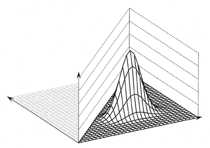
Figure 1. Representation of a Gaussian kernel, as represented by (2-1)
Figure 2 shows the values of wij with the exponent 2 replaced by 10. The weight function shows a very steep drop at distances a in the x–direction and b in the y–direction, with approximately the value 1 within the "frame" and zero outside the "frame." For larger values of the exponent, the drop becomes steeper, the frame narrower, and a moving average is approached. Therefore, (a x b) is called the size of the window. This is done for convenience since the actual size of the window is really ((2a) x (2b)).
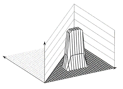
Figure 2. Representation of a Gaussian kernel with an exponent of 10.
Several choices have to be made when fitting a model. These include the density of the grid, the exponent, the size of the window, and the option of varying the orientation of the window. We experimented to determine which values of grid density and window size and orientation eliminated irregular waves and patterns, likely to be noise, but still retained features of the surface that may reflect real effects. Though statistical criteria can be developed, they are cumbersome, and we did not use them. We varied the grid size until a clear picture of a continuous surface was obtained visually. We also varied the window size until the surface appeared to be smooth, with only low local "waves." If the surface showed a "ridge" or similar pattern, we tried varying the orientation of the window. This, however, did little to reveal a pattern and we decided not to vary the orientation of the windows in this study.
The results of the smoothing process are shown as surfaces, formed by connecting the smoothed values at the grid points along the grid lines. The width of the lines is proportional to the number of cases in each cell. If the line was too narrow to be printable, it was printed as a dotted line. No grid lines are shown where there are no data points. Sometimes, a cell with no data points is surrounded by cells with data points. In that case two "sides" of adjacent cells will be seen through the "hole"' in the surface at the location of the cell with no data points.
Although there is some theoretical work on smoothing and a body of experimental work exists, additional development is desirable. For example, data points are usually not uniformly distributed over a surface. In areas covered densely with data points a small window suffices to average out the random variations, and reveal more details of the surface than a large window. However, in areas with sparse observations a large windows shows the general trend of the surface, but less detail. A procedure with adaptive window size, which would allow an analyst to make the best use of available information, still needs to be developed.
FHWA-RD-98-096
|


